Universidade de Brasília
Instituto de Ciências ExatasDepartamento de Ciência da Computação
Accelerating Sensitivity Analysis in Microscopy
Image Segmentation Workflows with Multi-level
Computation and Data Reuse
Willian de Oliveira Barreiros Júnior
Dissertação apresentada como requisito parcial para conclusão do Mestrado em Informática
Orientador
Prof. Dr. George Luiz Medeiros Teodoro
Brasília
2018
Ficha Catalográfica de Teses e Dissertações
Está página existe apenas para indicar onde a ficha catalográfica gerada para dissertações de mestrado e teses de doutorado defendidas na UnB. A Biblioteca Central é responsável pela ficha, mais informações nos sítios:
http://www.bce.unb.br
http://www.bce.unb.br/elaboracao-de-fichas-catalograficas-de-teses-e-dissertacoes
Universidade de Brasília
Instituto de Ciências ExatasDepartamento de Ciência da Computação
Accelerating Sensitivity Analysis in Microscopy
Image Segmentation Workflows with Multi-level
Computation and Data Reuse
Willian de Oliveira Barreiros Júnior
Dissertação apresentada como requisito parcial para conclusão do Mestrado em Informática
Prof. Dr. George Luiz Medeiros Teodoro (Orientador) CIC/UnB
Prof.a Dr.a Genaína Nunes Rodrigues Prof. Dr. Renato Antônio Celso Ferreira
CIC/UnB DCC/UFMG
Prof. Dr. Bruno Macchiavello
Coordenador do Programa de Pós-graduação em Informática
Dedicatória
Ao meu pai, que tomou como missão de vida apoiar-me de todas formas a seguir minha paixão nos estudos, e que embora não esteja mais aqui, continua a suceder.
Agradecimentos
Agradeço primeiramente à minha família pelo apoio nesta etapa da minha vida, aos com-panheiros de laboratório que me auxiliavam irrestritamente, e a meu orientador, George, que de alguma forma conseguiu suportar constantes interrupções minhas enquanto tentava me guiar.
Resumo
Com a crescente disponibilidade de equipamentos de imagens microscópicas médicas existe uma demanda para execução eficiente de aplicações de processamento de imagens Whole
Slide Tissue Images. Pelo processo de análise de sensibilidade é possível melhorar a qualidade dos resultados de tais aplicações, e subsequentemente, a qualidade da análise realizada a partir deles. Devido ao alto custo computacional e à natureza recorrente das tarefas executadas por métodos de análise de sensibilidade (i.e., reexecução de tarefas), emergem oportunidades para reuso computacional. Pela realização de reuso computa-cional otimiza-se o tempo de execução das aplicações de análise de sensibilidade. Este trabalho tem como objetivo encontrar novas maneiras de aproveitar as oportunidades de reuso computacional em múltiplos níveis de abstração das tarefas. Isto é feito pela apre-sentação de algoritmos de reuso de tarefas grão-grosso e de novos algoritmos de reuso de tarefas grão-fino, implementados no Region Templates Framework.
Palavras-chave: Reuso Computacional, Analise de Sensibilidade, Region Templates
Abstract
With the increasingly availability of digital microscopy imagery equipments there is a de-mand for efficient execution of whole slide tissue image applications. Through the process of sensitivity analysis it is possible to improve the output quality of such applications, and thus, improve the desired analysis quality. Due to the high computational cost of such analyses and the recurrent nature of executed tasks from sensitivity analysis methods (i.e., reexecution of tasks), the opportunity for computation reuse arises. By performing computation reuse we can optimize the run time of sensitivity analysis applications. This work focuses then on finding new ways to take advantage of computation reuse oppor-tunities on multiple task abstraction levels. This is done by presenting the coarse-grain merging strategy and the new fine-grain merging algorithms, implemented on top of the Region Templates Framework.
Sumário
1 Introduction 1 1.1 The Problem . . . 3 1.2 Contributions . . . 3 1.3 Document Organization . . . 4 2 Background 5 2.1 Microscopy Image Analysis . . . 52.2 Sensitivity Analysis . . . 6
2.3 Region Templates Framework (RTF) . . . 9
2.4 Related Work on Computation Reuse . . . 12
2.4.1 Computation Reuse Taxonomy . . . 12
2.4.2 Related Work Analysis . . . 14
3 Multi-Level Computation Reuse 19 3.1 Graphical User Interface and Code Generator . . . 21
3.2 Stage-Level Merging . . . 23
3.3 Task-Level Merging . . . 24
3.3.1 Naïve Algorithm . . . 25
3.3.2 Smart Cut Algorithm (SCA) . . . 25
3.3.3 Reuse Tree Merging Algorithm (RTMA) . . . 28
3.3.4 Task-Balanced Reuse-Tree Merging Algorithm (TRTMA) . . . 33
4 Experimental Results 44 4.1 Experimental Environment . . . 44
4.2 Impact of Multi-level Computation Reuse for Multiple SA Methods . . . 45
4.2.1 Impact of Multi-level Computation Reuse for MOAT . . . 45
4.2.2 Impact of Multi-level Computation Reuse for VBD . . . 46
4.3 SA Methods Reuse Analysis . . . 47
4.5 The Effect of the Merging on Scalability . . . 49 4.5.1 The Impact of Variable Task Cost . . . 51
5 Conclusion 53
Lista de Figuras
2.1 An example microscopy image analysis workflow performed before image classification. Image extracted from [2]. . . 5 2.2 An example of tissue image segmentation. . . 6 2.3 The main components of the Region Templates Framework, highlighting
the steps of a coarse-grain stage instance execution. Image extracted from [39]. . . 9 2.4 The execution of a stage instance from the perspective of a node, showing
the fine-grain tasks scheduling. Image extracted from [39]. . . 10 3.1 The parameter study framework. A SA method selects parameters of the
analysis workflow, which is executed on a parallel machine. The workflow results are compared to a set of reference results to compute differences in the output. This process is repeated a set number of times (sample size) with varying input parameters’ values. . . 19 3.2 A comparison of a workflow generated with and without computation reuse.
Image extracted from [42]. . . 20 3.3 An example stage descriptor Json file. . . 21 3.4 The example workflow described with the Taverna Workbench. . . 22 3.5 An example on which SCA executes on 5 instances of a workflow application
of 6 tasks, with M axBucketSize = 2. . . . 26 3.6 An example where node x is inserted on the existing reuse tree. Figure
3.6a defines the tasks of which each stage is composed by and presents the parameters’ values for each stage instance. . . 29 3.7 An example of Reuse Tree based merging with MaxBucketSize 3. The
merged stages of each step are shown below the tree on the bucket list. . . 30 3.8 Simple example of Full-Merge on which M axBuckets is 3 and the exact
division os stages is reached. . . 34 3.9 Another example of Full-Merge and Fold-Merge on which M axBuckets is
3.10 An example of a Fold-Merging of buckets b1-b6. Initially we start with
b = 6 buckets, trying to achieve M b = 4 buckets. In order to do so b − M b
merger operations are performed. The task cost of the buckets follows the ordering b1 ≥ b2 ≥ b3 ≥ b4 ≥ b5 ≥ b6. . . . 35 3.11 An example of the Balance step on which there are 3 buckets to be balanced. 36 3.12 A general worst-case reuse-tree representation on which we have all n stages
divided into b buckets. On this case we have b − 1 buckets with exactly one stage, and thus cost k. Hence, the last bucket has n − b + 1 stages. For this last bucket we assume the single and uniform reuse of the first r task, having no reuse for the remaining k − r tasks. This is the worst-case for balancing applications. . . 40 3.13 An example reuse-tree that can be used to illustrate possible prunable
nodes. E.g., the use of nodes 4, 5, 6, or 10, 11 as an improvement attempt results in the same outcome (cost 3), making them interchangeable, as with nodes 7, 8 or 9 (cost 4), or nodes 12-22 (cost 3). . . 41 3.14 Two examples of bad selection of smallRT using the last-bucket strategy. . 42 4.1 Impact of the computation reuse for different strategies as the sample size
of the MOAT analysis is varied. E.g., s150 means that the experiment had 150 executions of the given workflow. . . 45 4.2 Impact of the computation reuse strategies for the VBD SA method. . . . 47 4.3 Impact of varying M axBucketSize from 2 to 8. . . . 48 4.4 Comparison of the “no fine-grain reuse” (NR) approach with the RTMA
and TRTMA. RTMA uses M axBucketSize 10, while TRTMA uses M axBuckets 3× the number Worker Processes (WP). The execution times for WP > 32 were zoomed in a separated figure for the purpose of better visualization. . 49 4.5 Combination of Stages per Worker Processes (S/W) and parallelism
effi-ciency values. The S/W ratio for TRTMA was fixed as 3 for all WP values. The parallelism efficiency was calculated based on the previous execution (e.g. for WP 64, it is the execution time for WP 32 vs WP 64). . . 50 4.6 An example case on which two buckets with the same number of tasks
have different execution costs. This is due to the difference in the cost of different tasks. In this example Bucket 1 should execute 1.25× faster than Bucket 2. . . 52
Lista de Tabelas
2.1 Definition of parameters and range values: parameter space contains about 21 trillion points. . . 7 2.2 Example output of a MOAT analysis with all 15 parameters and a VBD
analysis with a selection of the 8 most influential parameters. The influence of a parameter is bounded in the interval [-1,1] and is proportional to its distance from 0 (i.e., 1 and -1 are the greatest values and 0 the smallest). . . 8 2.3 Taxonomic evaluation of computation reuse approaches. Implementation
Level (IL): Hardware (H) or Software (S). Application Flexibility (AF): Flex-ible, Partial or Domain Specific (DS). Reuse Strategy: Predictive, Memoiza-tion or Analytic. Task Granularity: InstrucMemoiza-tion-Level, Fine-Grain, Coarse-grain or Full Application. Reusable Tasks Matching: Same or Similar. Reuse Evaluation: Static or Dynamic. Needs Training Step (T). Reusability Envi-ronment Scale (RES): Local (L) or Distributed(D). . . 18 4.1 Maximum computation reuse potential for MC, LHS and QMC methods
with different sample sizes. For VBD, the number of experiments is 10 ×
SampleSize. The reuse percentages represent fine-grain reuse after
coarse-grain reuse, meaning that only fine-coarse-grain reuse is being shown. . . 48 4.2 Speedup of the TRTMA vs the “No Reuse” (NR) approach. . . 50 4.3 An empirical evaluation on the costs of each task of which a stage is
com-posed of. This approximation was generated with the purpose of showing the relative cost of the tasks, not being suitable as a absolute cost approximation. 51
Capítulo 1
Introduction
We define algorithm sensitivity analysis (SA) as the process of quantifying, comparing, and correlating output from multiple analyses of a dataset computed with variations of an analysis workflow using different input parameters [34]. This process is executed in many phases of scientific research and can be used to lower the effective computational cost of analysis on such researches, or even improve the quality of the results through parameter optimization.
The main motivation of this work is the use of image analysis workflows for whole slide tissue images analysis [20], which extracts salient information from tissue images in the form of segmented objects (e.g., cells) as well as their shape and texture features. Imaging features computed by such workflows contain rich information that can be used to develop morphological models of the specimens under study to gain new insights into disease mechanisms and assess disease progression.
A concern with automated biomedical image analysis is that the output quality of an analysis workflow is highly sensitive to changes in the input parameters. As such, adaptation of SA methods and methodologies employed in other fields [29, 48, 5, 16], can help understanding image analysis workflows for both developers and users. In short, the benefits of SA include: (i) better assessment and understanding of the correlation between input parameters and analysis output; (ii) the ability to reduce the uncertainty / variation of the analysis output by identifying the causes of variation; and (iii) workflow simplification by fixing parameters values or removing parts of the code that have limited or negligible effect on the output.
Although the benefits of using SA are many, its use in practice is limited given the data and computation challenges associated with it. For instance, a single study using a classic method such as MOAT (Morris One-At-Time) [29] may require hundreds of runs of the image analysis workflow (sample size). The execution of a single Whole Slide Tissue Image (WSI) will extract about 400,000 nuclei on average and can take hours on a single
computing node. A study at scale will consider hundreds of WSIs and compute millions of nuclei per run, which need to be compared to a reference dataset of objects to assess and quantify differences as input parameters are varied by the SA method. A single analysis at this scale using a moderate sample size with 240 parameter sets and 100 WSI would take at least three years if executed sequentially [39]. Given how time consuming such analysis is, there is a demand to develop mechanisms to make it feasible, such as parallel execution of tasks and computation reuse.
The information generated with a SA method is computed by executing or evaluating the same workflow as values of the parameters are systematically varied. As such, there are several parameters sets which have parameters with similar values. The workflows used on this work are hierarchical and, as such, can be broken down in routines, or fine-grained tasks. As such, it would be wasteful if one of these routines were to be executed on two or more evaluations generated by the SA method with the same parameters values and inputs. Thus, the re-executions of a given routine could reuse the results of the first execution in order to reduce the overall cost of the application.
Formally, computation reuse is the process of reusing routines or tasks results instead of re-executing them. Computation reuse opportunities arise when multiple computation tasks have the same input parameters, resulting in the same output, and thus making the re-execution of such task unnecessary. Computation reuse can also be classified by the level of abstraction of the reused tasks. Furthermore, these tasks can be combined on hierarchical workflows, with the routines and sub-routines of which they are composed by, being able to be fully or partially reused. Seizing reuse opportunities is done by a merging process, in which two or more tasks are merged together, after which the repeated or reusable portions of the merged tasks are executed only once.
Computation reuse on this work will be accomplished with the use of finer-grain tasks merging algorithms, as opposed to the already existing coarser-grain merging method implemented on the Region Templates Framework (RTF) platform, on which all algo-rithms are implemented on. This platform is responsible for the distributed execution of hierarchical workflows in large-scale computation environments.
Other works have studied computation reuse as a means to reduce overall computa-tional cost in different ways [30, 36, 32, 47, 28, 37, 17, 18]. Although the principle of computation reuse is rather abstract, its implementation on this work is distinct from existing methods. Some of these methods resort to hardware implementations [36, 32], which are not general or flexible enough for the given problem. Some apply reuse by pro-filing the application [47], which is also impracticable on the SA domain. Finally, most of them rely on caching systems of distinct levels of abstraction to reduce the overall cost of the applications [28, 37, 17, 18], being too expensive to employ on the desired scale of
distribution.
Summarizing, this work focuses on two ways of accomplishing computation reuse in SA applications for the RTF: (i) coarse-grain tasks reuse and (ii) fine-grain tasks reuse. The main differences between them, besides the granularity of the tasks to be reused, are the underlying restrictions of the system used to execute these tasks. The reuse of coarse-grain tasks can offer a greater speedup when reuse happens, but there are less reuse opportunities. With fine-grain tasks these reuse opportunities are more frequent, however, more sophisticated strategies need to be employed in order to deal with dependency resolution and to avoid performance degradation due to the impact of excessive reuse to the parallelism.
1.1
The Problem
Because of high computing demands, sensitivity analysis applied to microscopy image analysis is unfeasible for routinely use when applied to whole slide tissue images.
1.2
Contributions
This work focuses on improving the performance of SA studies in microscopy image anal-ysis through the application of finer-grain computation reuse on top of the coarse-grain computation reuse.
The specific contributions of this work are presented below with a reference to the section in which they are described:
1. A graphical user interface for simplifying the deployment of workflows for the RTF, which is coupled with a code generator that allows the flexible use of the RTF on distinct domains [Section 3.1];
2. The development and analysis of multi-level reuse algorithms:
(a) A coarse-grain merging algorithm was implemented [Section 3.2];
(b) A fine-grain Naïve Merging Algorithm was proposed and implemented [Section 3.3.1];
(c) The fine-grain Smart Cut Merging Algorithm was proposed and implemented [Section 3.3.2];
(d) The fine-grain Reuse-Tree Merging Algorithm was proposed and implemented [Section 3.3.3];
3. Proposal and implementation of the Task-Balanced Reuse-Tree Merging Algorithm that reduces the issue of loss of parallelism due to load imbalance provoked by the Reuse-Tree Merging Algorithm [Section 3.3.4];
4. The performance gains of the proposed algorithms with a real-world microscopy im-age analysis application were demonstrated using different SA strategies (e.g MOAT and VBD) at different scales.
The contributions of Sections 3.1, 3.2 and 3.3.3 were published on the IEEE Cluster 2017 conference [2], comprising, but not restricted to the proposal of multi-level compu-tational reuse, the proposal of the Reuse-Tree structure for fine-grain merging and the experimental results for lower scale tests. Moreover, the contributions of Section 3.3.4 are currently being drafted for a submission for a journal publication. These contribu-tions, which are an extension of the published work [2], includes some further analysis of computation reuse within the scope of scalability under more challenging settings, some limitations of the previously proposed solution for fine-grain merging, and finally, a new approach to cope with such limitations.
1.3
Document Organization
The next section describes the motivating application, the theory behind computation reuse and the Region Templates Framework (RTF), which was used to deploy the appli-cation on a parallel machine and is also the tool in which the merging algorithms were incorporated. After these considerations more relevant related work is analyzed. Section III describes the proposed solutions for multi-level computation reuse, their implementa-tions and optimizaimplementa-tions. On Section IV the experimental procedures are described and the results are analyzed. Finally, Section V closes this work with contributions and possible future goals for its continuation.
Capítulo 2
Background
This chapter describes the motivating application along with the Region Templates Frame-work, in which this work is developed, and some basic concepts of sensitivity analysis and computation reuse. Being the contributions of this work restricted to computation reuse, this chapter then ends with the analysis of some relevant related work on the subject.
2.1
Microscopy Image Analysis
It is now possible for biomedical researchers to capture highly detailed images from whole slide tissue samples in a few minutes with high-end microscopy scanners, which are becom-ing evermore available. This capability of collectbecom-ing thousands of images on a daily basis extends the possibilities for generating detailed databases of several diseases. Through the investigation of tissue morphology of whole slide tissue images (WSI) there is the possibility of better understanding disease subtypes and feature distributions, enabling the creation of novel methods for classification of diseases. With the increasing number of research groups working and developing richer methods for carrying out quantitative mi-croscopy image analyses [14, 31, 23, 9, 12, 7, 8, 26] and also the increasingly availability of digital microscopy imagery equipment, there is a high demand for systems or frameworks oriented towards the efficient execution of microscopy image analysis workflows.
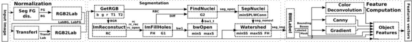
Figura 2.1: An example microscopy image analysis workflow performed before image classification. Image extracted from [2].
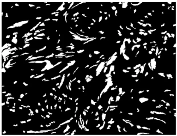
(a) A tissue image. (b) The segmented tissue image.
Figura 2.2: An example of tissue image segmentation.
The microscopy image analysis workflow used on this work is presented in Figure 2.1 and was proposed by [21, 22, 44]. This workflow consists of normalization (1), seg-mentation (2), feature computation (3) and final classification (4), being the first three analysis stages the most computationally expensive phases. The first stage is responsible for normalizing the staining and/or illumination conditions of the image. The segmenta-tion is the process of identifying the nucleus of each cell of the analyzed image (Figure 2.2). Through feature computation a set of shape and texture features is generated for each segmented nucleus. At last, the final classification will typically involve using data mining algorithms on aggregated information, by which some insights on the underlying biological mechanism that enables the distinction of subtypes of diseases are gained.
The quality of the workflow analysis is, however, dependent of the quality of the parameters values, with them described in Table 2.1. Therefore, in order to improve the effectiveness of the analysis the impact of these parameters on the output of the used workflow (Figure 2.1) should be analyzed. This impact analysis is known as sensitivity analysis and is detailed on the following section.
2.2
Sensitivity Analysis
We define Sensitivity Analysis (SA) as the process of quantifying, comparing and correlat-ing the input parameters of a workflow with the intent of quantifycorrelat-ing the impact of each input to the final output of the workflow [34]. This process is applied on several phases of scientific research including, but not limited to model validation, parameter studies and optimization, and error estimation [33]. The outcome of such methods, as defined in [42], are statistics that quantify variance in the analysis results as well as measures such as
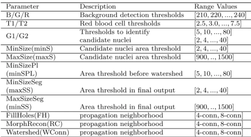
Parameter Description Range Values B/G/R Background detection thresholds [210, 220, ..., 240] T1/T2 Red blood cell thresholds [2.5, 3.0, ..., 7.5] G1/G2 Thresholds to identify [5, 10, ..., 80]
candidate nuclei [2, 4, ..., 40] MinSize(minS) Candidate nuclei area threshold [2, 4, ..., 40] MaxSize(maxS) Candidate nuclei area threshold [900, .., 1500] MinSizePl
(minSPL) Area threshold before watershed [5, 10, ..., 80] MinSizeSeg
(maxSS) Area threshold in final output [2, 4, ..., 40] MaxSizeSeg
(minSS) Area threshold in final output [900, .., 1500] FillHoles(FH) propagation neighborhood [4-conn, 8-conn] MorphRecon(RC) propagation neighborhood [4-conn, 8-conn] Watershed(WConn) propagation neighborhood [4-conn, 8-conn]
Tabela 2.1: Definition of parameters and range values: parameter space contains about 21 trillion points.
sensitivity induces that indicate the amount of variance in the analysis results that can be attributed to individual parameters or combinations of parameters.
Usually, the computational cost for performing SA on a workflow is directly propor-tional to the number of parameters it has. One way to simplify the analysis on applica-tions with large numbers of parameters, thus reducing its cost, is through the removal of parameters whose effect on the output is negligible.
This work focuses on using the already existing system, the Region Templates Frame-work (RTF) [39, 42], which performs sensitivity analysis in two phases. On the first phase the 15 input parameters (Table 2.1) are screened with a light, or less compute demanding, SA method, used to remove the so called non-influential parameters from the next phase. Afterwards, a second SA method is executed on the remaining parameters, on which both first-order and high-order effects of these on the application output are quantified. This two-phase analysis is performed since the cost of more specific approaches (e.g., VBD) are prohibitively expensive.
This multi-phase sensitivity analysis process is approached on [33] as an alternative to cope with costly analysis. The application case, as seen in Figure 2.1 uses a complex model with several input parameters (see Table 2.1) and a high execution cost. As such, it is recommended that a lighter preliminary analysis method should be executed on the full range of input parameters, only to reduce these to a smaller subset of important parameters. As a way to further reduce the analysis complexity on this first screening analysis is to also drop inputs’ correlation analysis. After the execution of a screening method, more complex and comprehensive analysis methods can be performed on a subset of the input parameters. The chosen SA methods for this work were Morris One-At-A-Time as a screening method [29], and Variance-Based Decomposition as a more complete analysis.
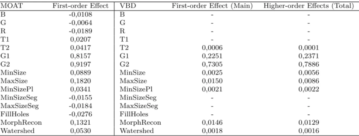
MOAT First-order Effect VBD First-order Effect (Main) Higher-order Effects (Total) B -0,0108 B - -G -0,0064 G - -R -0,0189 R - -T1 0,0207 T1 - -T2 0,0417 T2 0,0006 0,0001 G1 0,8157 G1 0,2251 0,2371 G2 0,9197 G2 0,7305 0,7886 MinSize 0,0889 MinSize 0,0025 0,0056 MaxSize 0,1820 MaxSize 0,0150 0,0086 MinSizePl 0,0341 MinSizePl 0,0021 0,0022 MinSizeSeg -0,0155 MinSizeSeg - -MaxSizeSeg -0,0184 MaxSizeSeg - -FillHoles -0,0276 FillHoles - -MorphRecon 0,1321 MorphRecon 0,0146 0,0129 Watershed 0,0530 Watershed 0,0018 0,0016
Tabela 2.2: Example output of a MOAT analysis with all 15 parameters and a VBD analysis with a selection of the 8 most influential parameters. The influence of a parameter is bounded in the interval [-1,1] and is proportional to its distance from 0 (i.e., 1 and -1 are the greatest values and 0 the smallest).
The light SA method, Morris One-At-A-Time (MOAT) [29], performs a series of runs of the application changing each parameter individually, while fixing the remaining pa-rameters in a discretized parameter search space. Each of the k analyzed papa-rameters values ranges are uniformly partitioned in p levels, thus resulting in a pk grid of parame-ter sets to be evaluated. Each evaluation output xi of the application creates a parameter
elementary effect (EE), calculated as EEi = y(x1,...,xi+∆∆i,...,xk)−y(x)
i , with y(x) being the
application output before the parameter perturbation. In order to account for global SA the RTF uses ∆i = 2(p−1)p [42]. The MOAT method requires r(k + 1) evaluations, with r
in the range of 5 to 15 [15].
The second SA method, Variance-Based Decomposition (VBD) is preferably performed after a lighter SA screening method, as the MOAT method. This is done since VBD requires n(k + 2) evaluations for k parameters and n samples, with n lying in the order of thousands of executions [48]. Thus, it is interesting to use a reduced number of parameters for feasibility reasons. VBD, unlike MOAT, discriminates the the output uncertainty effects among individual parameters (first-order) and high-order effects.
As an example, Table 2.2 provides the expected outcome of a two-steps SA of the used workflow. The first analysis, MOAT, is performed at an earlier moment in order to screen all parameters regarding their first-order effects or influence over the output. Afterwards, the VBD analysis can be performed with a subset of the 8 most influential parameters, yielding not only more precise first-order effect values but also a way to calculate higher-order effects through the manipulation of the Total values (e.g., for a third-higher-order effect of T2, G1 and G2, their Total values are added together and compared with the remaining
Regardless of the SA method chosen, the use of large set of parameters (Table 2.1) results in the unpractical task of performing SA on the workflow of Figure 2.1 due to the expected cost of evaluating such large search domain. For the sake of mitigating this infeasibility issue for performing SA on the presented workflow we can execute the analysis on high-end distributed computing environments. Also, computation reuse can be employed to reduce the computational cost without the need of application specific optimizations. Both mentioned methods are described in the next sections.
2.3
Region Templates Framework (RTF)
The Region Template Framework (RTF) abstracts the execution of a workflow application on distributed environments [39]. It supports hierarchical workflows that are composed of coarse-grain stages, which in turn are composed by fine-grain tasks. The dependencies between stages, and tasks of a single stage are solved by the RTF. Given a homogeneous environment of n nodes with k cores each, any stage instance must be executed on a single node, with its tasks being executed on any of the k cores of the same node. It is noteworthy that, not only any node can have more than one stage instance executing on
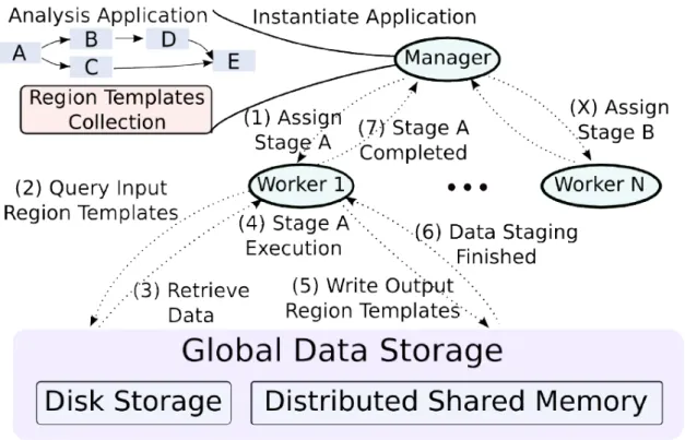
Figura 2.3: The main components of the Region Templates Framework, highlighting the steps of a coarse-grain stage instance execution. Image extracted from [39].
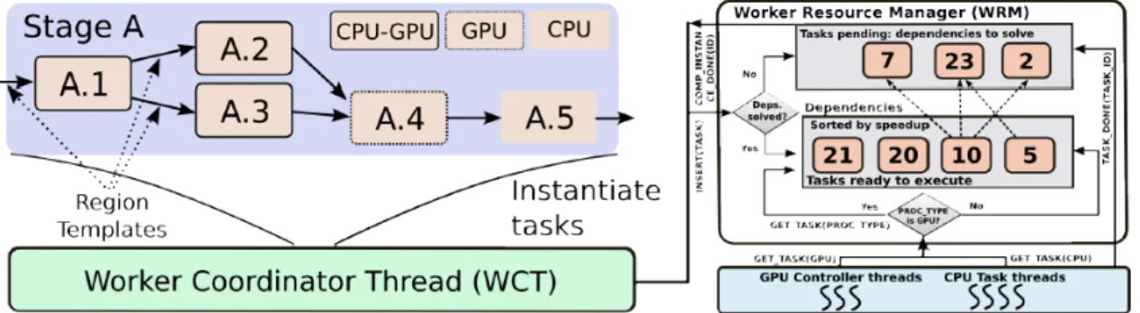
Figura 2.4: The execution of a stage instance from the perspective of a node, showing the fine-grain tasks scheduling. Image extracted from [39].
it, but also, there may be more than one task from the same stage running in parallel, given that the inter-tasks dependencies are respected.
The main components of the RTF are: the data abstraction, the runtime system, and the hierarchical data storage layer [39]. The runtime system consists of core functions for scheduling of application stages, transparent data movement and management via the storage layers. Figure 2.3 shows an example of the dispatch of a stage to a worker with the data exchanges in the RTF storage layer. The RTF, with its centralized Manager, distributes the stages to be executed to Worker nodes across the network. The hierarchical workflow representation allows for different scheduling strategies to be used at each level (stage-level and task-level). Fine-grain scheduling is possible at task-level in order to also exploit variability in performance of application operations in hybrid systems. In Figure 2.4 a stage A is sent to a worker node for execution, which tasks are scheduled locally.
Still on the scheduler, the Manager schedules stages to Workers on a demand-driven basis, with the Workers requesting work from the Manager until all stages are executed. Since the Worker decides when they request more work, a Worker can execute one or more stage at any given time instant, based on its underlying infrastructure. Being a stage composed of tasks, these are scheduled locally by the Worker executing them. These tasks differ in terms of data access patterns and computation intensity, thus, attaining different speedups if executed on co-processors or accelerators. In order to optimize the execution of tasks a Performance Aware Task Scheduling (PATS) was implemented [39, 44, 41, ?, 45, 11, 40, 43]. With PATS, tasks are assigned to either a CPU or GPU core based on its estimated acceleration and the current device load.
On the data storage layer the Region Templates (RT) data abstraction is used to represent and interchange data (represented by the collection of objects of an application instance and the stored data of Figure 2.3). It consists of storage containers for data structures commonly found in applications that process data in low-dimensional spaces (1D, 2D or 3D spaces) with a temporal component. The data types include: pixels, points,
arrays (e.g., images or 3D volumes), segmented and annotated objects and regions, all of which are implemented using the OpenCV [4] library interfaces to simplify their use. A RT data instance represents a container for a region defined by a spatial and temporal bounding box. A data region object is a storage materialization of data types and stores the data elements in the region contained by a RT instance, which may have multiple data regions.
Access to the data elements in data regions is performed through a lightweight class that encapsulates the data layout, provided by the RT library. Each data region of one or multiple RT instances can be associated with different data storage implementations, defined by the application designer. With this design the decisions regarding data move-ment and placemove-ment are delegated to the runtime environmove-ment, which may use different layers of a system memory to place the data according to the workflow requirements.
The runtime system is implemented through a Manager-Worker execution model that combines a bag-of-tasks execution with workflows. The application Manager creates in-stances of coarse-grain stages, and exports the dependencies among them. These depen-dencies are represented as data regions to be consumed/produced by the stages. The assignment of work from the Manager to Worker nodes is performed at the granularity of a stage instance using a demand-driven mechanism, on which each Worker node indepen-dently requests stages instances from the Manager whenever it has idle resources. Each node is then responsible for fine-grain task scheduling of the received stage(s) to its local resources.
To create an application for the RTF the developer needs to provide a library of domain specific data analysis operations (in this case, microscopy image analysis) and implement a simple startup component that generates the desired workflow and starts the execution. The application developer also needs to specify a partitioning strategy for data regions encapsulated by the region templates to support parallel computation of said data regions associated with the respective region templates.
Stages of a workflow consume and produce Region Template (RT) objects, which are handled by the RTF, instead of having to read/write data directly from/to stages or disk. While the interactions between coarse-grain stages are handled by the RTF, the task of writing more complex, fine-grained, stages containing several external, domain specific, fine-grain API calls is significantly harder for application experts. This occurs since the RTF works only with one type of task objects as its runnable interface, not providing an easy way to compose stages using fine-grain tasks. The RTF also supports efficient execution on hybrid systems equipped with CPU and accelerators (e.g, GPUs).
2.4
Related Work on Computation Reuse
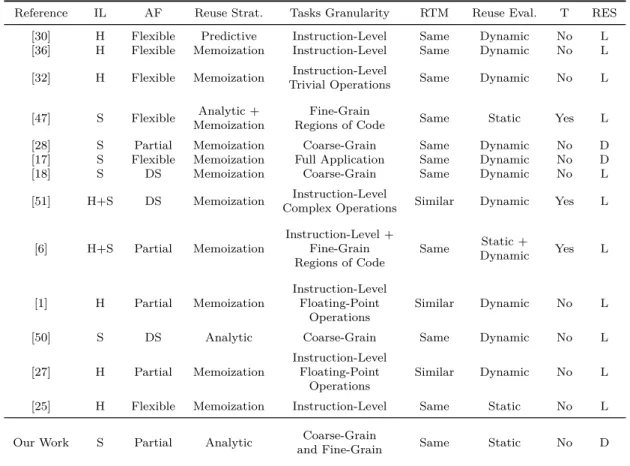
The idea of work reuse, also known as value locality [6, 25], has been employed on both the hardware and software fronts with diverse techniques, such as value prediction [30], dynamic instruction reuse [36] and memoization [32], with the goal of accelerating appli-cations through the removal of duplicated computational tasks. This concept has been used for runtime optimizations on embedded systems [47], low-level encryption value gen-eration [28] and even stadium designing [37]. In order to further analyze these existing approaches as to find desirable features that solve the problem approached in this work a qualitative analysis was performed, which is summarized on Table 2.3. This analysis uses taxonomic terms defined here to classify computation reuse approaches. The proposed taxonomic terminology is explained on the next section in addition to a brief analysis of each of the studied computation reuse approaches.
2.4.1
Computation Reuse Taxonomy
Implementation Level (IL)
Computation reuse can be enforced on either Software (S) or Hardware (H) levels. By
Software-Level it is meant a hardware-independent approach that can either be executed as
a static analysis before the execution of any computational task, or as a runtime approach that performs computation reuse as the application is executed. Also, it is possible for computation reuse to be searched on compilation-time by a customized compiler, which is also defined as Software-Level. It is also possible for these techniques to be combined.
Application Flexibility
Here we define the Application Flexibility(AF) of an approach as either General, Partial or Domain Specific (DS). A General approach is any that does not have domain-specific restrictions that limits or prevents its use on different domains. The flexibility of an approach can also be Partial, meaning that either some non-trivial adaptations need to be employed or that anything outside its application domain will execute rather poorly. If an approach can only be used on a rather specific environment, or under strict restrictions it is said to be a Domain Specific approach.
Reuse Strategy
One of the most important computation reuse characteristics is how computation reuse opportunities are found and explored. These can be defined as Predictive, Memoization or Analytic approaches. Computation reuse can be attained through the speculative
technique of Value Prediction [36, 6] with its implementations relying on a buffer that contains the results of previous instructions executions, with which the value prediction is performed.
The most common technique for computation reuse is through Memoization, which is a cache-based approach on which reusable tasks results are stored on a buffer for later reuse. It is worth noting that the stored values are used as-is, unlike with Value Prediction, which relies on the evaluation of the buffered values in order to return a reusable value. This approach has the drawback of needing a buffer structure, which increases the complexity of this kind of solution.
The alternative to Memoization is to find all reuse opportunities in an Analytic manner. This means that the reused tasks were found a priori, instead of searching the results in a buffer as with the Memoization scheme. While this approach is considered to be the one with the least overhead, such analysis is more difficult to be achieved.
Tasks Granularity
Still another rather important aspect of computation reuse is the Granularity of the reusable tasks. On this work we break Task Granularity in four categories:
Instruction-Level (i.e., CPU instruction), Fine-Grain Subroutines, Coarse-Grain Routines and Full Application. We differentiate Fine-Grain from Coarse-Grain tasks by their semantical
meaning, and as a consequence, their overall cost. If a task is big enough to have a broader meaning (e.g., a segmentation operation) we call it a Coarse-Grain Routine. If the task is bigger than a CPU instruction but also not big enough to have a more abstract meaning (e.g., the preparation of a matrix on memory, or a set of loops on an algorithm) we define them as Fine-Grain Subroutines or tasks. Finally, some approaches may only be able to work with a Full Application execution.
The importance of the granularity for computation reuse is that it limits the maximum amount of reuse of any application. As an example we have a segmentation algorithm. If we were to break it in CPU instructions and then perform a complete search for reusability (i.e., search for all available reuse) we would attain the maximum possible reuse. However, the potential overhead for exploiting this level of reuse is high. By grouping this low-level operations into subroutines we reduce the number of tasks, making the search for reuse more feasible. This grouping would also hide some reuse opportunities, effectively reducing the reuse potential of the application.
Reusable Tasks Matching (RTM)
An easy way to improve the reuse degree of an application is by relaxating the matching constraint for reuse. By doing this, reuse is possible even if not all tasks’ parameters
match, unlike the most common case on which all tasks’ parameters are the Same. The obvious consequence of doing this relaxation is that the tasks’ results will be different. However, some applications can deal with small imprecisions of its tasks (e.g., neural networks, multimedia applications, floating-point operations). As such, given that these partial (or Similar) matchings respect the precision necessary for these applications which can cope with such imprecisions, this strategy can improve the amount of reuse available.
Reuse Evaluation
Computation reuse can be analyzed either Dynamically, at runtime, of Statically before the execution of any task.
Training Required (T)
Approaches that rely on domain-specific characteristics of applications (e.g., neural net-works) usually require a Training step before the reuse analysis. For these approaches it is important to be mindful of the Training cost.
Reusability Environment Scale (RES)
The reusable tasks scope is defined here as the Reusability Environment Scale. The tasks can be reusable among a Distributed (D) environment of computing nodes or reused only
Locally (L).
2.4.2
Related Work Analysis
Sodani and Sohi [36] motivate their work by drawing a parallel of a computation reuse
buffer used to optimize instruction execution with memory cache used to optimize memory
access instructions. Their approach aims to reduce computational cost through reuse by (i) ending the instruction pipeline earlier, thus also reducing resources conflicts, and (ii) by breaking dependencies of later instructions, which can be executed earlier since the necessary inputs are already present. They initially proposed their reuse buffer as a way to reduce branch misprediction penalties. However, the effectiveness of this approach proved itself much more powerful since the reuse frequency of other, more generic, types of instructions also proved to be high. Their implementation focus on adding a reuse
buffer to any generic dynamically-scheduled superscalar processor, using one of the three
instruction reuse schemes proposed by them.
The approach on [36] can be used for any application domain while also being exposed to the largest possible amount of reuse opportunities. Their incorporation of the reuse
thus having no negative impact on non-reused instructions. Nevertheless, the efficiency of all instruction reuse schemes are heavily reliant on the buffer size. Although the used buffer sizes tested by them are small, this dependency is a limiting factor for the approach since smaller buffers means less reuse opportunities. Finally, the use of a hardware-based approach limits its use even further given the difficulty to design a processor for this sole purpose.
The work on [32], similarly to [36], also uses hardware-level memoization, but this time with a subset of operations called trivial computation. These are potentially complex operations that are trivialized by simple operands (e.g., integer division by two). This strategy greatly simplifies the reuse protocol (i.e., whether an instruction is reused, inser-tion and replacement policies) at the cost of reuse opportunities. The speedups achieved by this approach were only significant when the application was favorable to the reuse strategy (e.g., Ackerman-like applications with huge amounts of trivial operations, or floating-point-intensive programs, which have naturally long-latency instructions). The same limitations of [36] were present here as well.
Wang and Raghunathan [47] attempt to reduce the energetic cost of embedded software on battery-powered devices through a profiling-based reuse technique with a memoization structure. Some interesting discussions risen in their work regard reusable tasks granu-larity and the limitations of hardware-based reuse. Hardware implementations of compu-tation reuse are usually complex, and the use of overly fine-grained operations for reuse may yield little or negative speedups given the overhead of memoization caches.
The methodology of [47] consists on profiling an application, generating computation
reuse regions, setting the software cache configuration, evaluating the energy expenditure
and then doing it all over again until a good enough solution is found. Only then, the optimized application is sent to production. The concept of flexible computation reuse
regions is very powerful since it makes the application more domain-independent while
also optimizing the granularity of the reuse for any application instance. Their automated software cache configuration is also interesting since any memoization-based technique is heavily reliant on its size and performance.
Unfortunately [47] do not specify the cost of profiling (since for the test environment the typical input traces of the selected benchmarks were already available), nor the cost of configuring the computation reuse regions and the software cache. Regardless, this ap-proach, while presenting the concepts of flexible granularity and automatic software cache configuration / optimization, cannot be recommended for large-scale workflow execution given its unknown-cost training step. Also, in order to distribute the computation reuse, the software cache used by it needs to be re-thought to be compatible with this paradigm. It is brought to our attention on [28] the cost of two-party secure-function evaluation
(SFE) and the tendency to offload these operations from resource-constrained devices to outside servers. In order to reduce the computational cost of these SFE operations as well as bandwidth requirements, a system on which state is retained as to later be reused was implemented. The reusable encrypted values can be used by a number of clients on a distributed setting, originating from a centralized server node that implements a
memoization buffer.
Although [28] is the first approach to enable computation reuse to be done in a dis-tributed environment, the encrypted values buffer is a bottleneck for the approach scal-ability. In order to remove this bottleneck, the buffer can be distributed among server nodes, which has as a consequence either (i) the buffers are coherent, and as such the servers need to keep trading messages to enforce it, or (ii) the buffers are not coherent and thus the reuse potential is reduced. Finally, this approach is only partially applicable for different application domains since the granularity of the reused tasks must be rather coarse in order to achieve good speedups. This happens because the of the big overhead of reusing encrypted values.
Approach [17] also works with distributable reusable values, but this time with bioin-formatics applications, which are known to be computationally expensive. The granularity of reusable tasks is even coarser, being able to perform full end-to-end reuse of workflows. When comparing with [28], [17] has the same limitations given its memoization-based approach.
On [18] Santos and Santos propose the use of a software-level runtime buffer system to cache and then reuse energy evaluations for predicting the native conformation of proteins. The domain-specific application relies on a genetic algorithm, and as such, their approach is tailored for this single application. A similar approach is the one of Yasoubi et al. [51], regarding the use of memoization-based computation reuse, optimized for a specific domain, which is neural networks on this case.
Yasoubi et al. [51] propose an offload hardware accelerator that uses clustered groups of neurons that maximize the expected computation reuse when executing the application. It is worth noting that the clustering is done by a k-means algorithm on software level. The reusable tasks are hardware-level multiplication instructions that, given the multi-processing-unit (multi-PU) architecture, disable PUs that perform repetitive operations, thus reducing the power consumption.
The work of Connors and W.Hwu [6] exploit value locality through the combination of a hardware buffer, an instruction set for representing different-sized reusable computa-tional tasks and a profile-guided compiler that groups instructions into reusable tasks as to optimize their granularity. This approach was implemented as a way to extend hardware-only-based reuse approaches while solving the limitation of instruction-level reusable tasks
granularity. Again, the use of dynamically-sized reusable tasks makes the approach more flexible to different domains of applications while optimizing the reusable tasks granu-larity for each application instance. However, in order to implement this feature the approach on [6] limits itself by needing a complex hardware and compiler implementation and profiling information on the domain-specific application.
Álvarez et al. [1] focus on reducing the power consumption of low-end and/or mobile devices by applying computation reuse on multimedia applications. This is done by exploiting the imprecision tolerance of multimedia floating-point operations at hardware-level to reuse tasks that are similar enough, thus increasing the amount of attainable computation reuse. Nonetheless, this “similar enough” strategy limits the usability of this approach to multimedia applications, or applications which have a large number of floating-point reusable operations. The same is true for approach [27], which in turn proposes a more generic implementation that was not tailored for multimedia applications. The first analytic computation reuse method is presented by Xu et al., on [50]. On their work they propose a framework for Isogeometric Analysis (IGA) that reuse matrix calculations. The reuse operations were statically analyzed a priori and are specific of IGA, meaning that this approach, although having good speedups, cannot be applied for other application domains.
Lepak and Lipasti [25] propose reuse of memory load instructions. This is done through the characterization of value locality for memory instructions and the implementations of two reuse protocols for both uniprocessed and multiprocessed environments. For unipro-cessed systems reuse can be attained by either analyzing the value locality of specific instructions (based on the program structure), or the locality of a particular memory address (message-passing locality). Furthermore, they define silent stores as stores oper-ations that do not change the system state (i.e., the written value is the same as the one previously present on memory). Given some statistical analysis of how many silent stores are on selected benchmarks, they set an ideal maximum reuse possible to be achieved and, through their proposed protocols, aim to get as close as possible to these values.
Since none of the previous applications is either compatible or flexible enough to work on the large scale bioinformatics workflows application domain, this work proposes a novel approach to computation reuse. The proposed approach works with software-level reuse, since it is being implemented on top of the RTF. Also, given that this application is supposed to be executed on a large-scale cluster environment, hardware-based approaches are impractical. Moreover, the runtime system must be light in order to execute on a large-scale distributed environment, thus making the use of memoization impractical. Given that the application uses hierarchical workflows, any applications of other domains need to be converted to workflows in order to be executed by our approach, slightly impacting
Reference IL AF Reuse Strat. Tasks Granularity RTM Reuse Eval. T RES [30] H Flexible Predictive Instruction-Level Same Dynamic No L [36] H Flexible Memoization Instruction-Level Same Dynamic No L [32] H Flexible Memoization Instruction-Level
Trivial Operations Same Dynamic No L
[47] S Flexible Analytic + Memoization
Fine-Grain
Regions of Code Same Static Yes L [28] S Partial Memoization Coarse-Grain Same Dynamic No D [17] S Flexible Memoization Full Application Same Dynamic No D [18] S DS Memoization Coarse-Grain Same Dynamic No L [51] H+S DS Memoization Instruction-Level
Complex Operations Similar Dynamic Yes L
[6] H+S Partial Memoization Instruction-Level + Fine-Grain Regions of Code Same Static + Dynamic Yes L [1] H Partial Memoization Instruction-Level Floating-Point Operations Similar Dynamic No L
[50] S DS Analytic Coarse-Grain Same Dynamic No L
[27] H Partial Memoization
Instruction-Level Floating-Point
Operations
Similar Dynamic No L
[25] H Flexible Memoization Instruction-Level Same Static No L
Our Work S Partial Analytic Coarse-Grain
and Fine-Grain Same Static No D
Tabela 2.3: Taxonomic evaluation of computation reuse approaches. Implementation Level (IL): Hardware (H) or Software (S). Application Flexibility (AF): Flexible, Partial or Domain Specific (DS). Reuse Strategy: Predictive, Memoization or Analytic. Task Granularity: Instruction-Level, Fine-Grain, Coarse-grain or Full Application. Reusable Tasks Matching: Same or Similar. Reuse Evaluation: Static or Dynamic. Needs Training Step (T). Reusability Environment Scale (RES): Local (L) or Distributed(D).
the application domain flexibility. Finally, computation reuse is achievable by a static analytic analysis of reuse before the execution of any task, thus removing any distribution limitations as long as the reuse analysis can be performed quickly.
Capítulo 3
Multi-Level Computation Reuse
This work has as its main goal the development of Sensitivity Analysis (SA) optimizations through multi-level computation reuse. This chapter analyzes computation reuse and then describes improvements made to the Region Templates Framework (RTF), which were implemented in order to enable the use of multi-level computation reuse. After that, the new computation reuse approaches are described, along with their advantages and disadvantages.
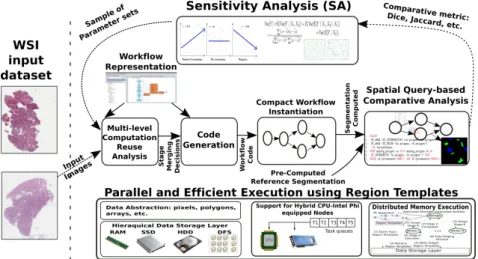
The SA studies and components that were developed and integrated into the RTF are illustrated in Figure 3.1. An SA study in this framework starts with the definition of a given workflow, the parameters to be studied, and the input data. The workflow is then instantiated and executed efficiently in RT using parameters values selected by the SA method. These values, or parameters sets, are generated separately by the user through
Figura 3.1: The parameter study framework. A SA method selects parameters of the analysis workflow, which is executed on a parallel machine. The workflow results are compared to a set of reference results to compute differences in the output. This process is repeated a set number of times (sample size) with varying input parameters’ values.
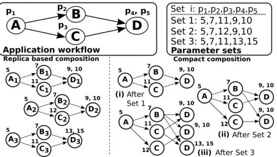
Figura 3.2: A comparison of a workflow generated with and without computation reuse. Image extracted from [42].
a SA method statically, i.e, before the execution of any task on the RTF. The output of the workflow is compared using a metric selected by the user to measure the difference between a reference segmentation result and the one computed by the workflow using the parameter set generated by the SA method. This process continues while the number of workflow runs does not achieve the sample size required by the SA. This sample size is effectively the number of times that the workflow will be instantiated and executed with different input parameters’ values. The sample size is a way to limit the cost of the SA study while maintaining its significance and accuracy. This can be done by empirically choosing a sample size that is big enough to have accurate results but not enough that its cost is unfordable.
Computation reuse is achieved through the removal of repeated computation tasks. Figure 3.2 presents the comparison of a replica-based workflow generation, in which there is no reuse, and a compact composition, generated with maximal reuse. Given that we start generating a compact composition with no tasks on it, the first parameter set (Set 1, (i) in Figure 3.2) is added to the workflow in its entirety (i.e., all computation tasks A-D). The second parameter set, however, has the reuse opportunities of tasks A and B given they have the same input parameters values and input data. Thus, only the tasks C and D for parameter set 2 are instantiated in the compact graph ((ii) in Figure 3.2). With the current workflow state of (ii), parameter set 3 presents reuse opportunities for tasks A, B and C, thus only needing to instantiate a single computation task (D) with the parameters values 13 and 15 to the workflow. When comparing the workflow replica based composition with the compact composition we can notice a decrease on the number of executed tasks of approximately 41%, from 12 tasks to 7 tasks.
There are two computation reuse levels used on this work, (i) stage-level, on which coarse-grain computation tasks are reused, and (ii) task-level - with fine-grain tasks reused. Coarse-grain computation reuse is significantly easier to implement than its fine-grained counterpart. However, the number of parameters that two coarse-grained merging candi-dates stages need to match for the reuse to take place is higher as when compared with fine-grain tasks.
3.1
Graphical User Interface and Code Generator
In this work a flexible task-based stage code generator was implemented to ease the process of developing RTF applications. This generator was created, together with a workflow generator graphical interface - with the purpose of making the RTF more accessible to domain-specific experts. Additionally, this code generator will simplify the application information gathering process, necessary for merging stages instances during the process of computation reuse.
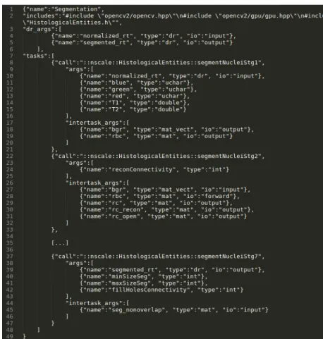
The stage generator has as its input a stage descriptor file, formatted as Json, as shown in Figure 3.3. A stage is defined by its name, the external libraries it needs to call in
Figura 3.4: The example workflow described with the Taverna Workbench.
order to execute the application domain transformations in each stage of the workflows, the necessary input arguments for its execution and the tasks it must execute. There are two kinds of inputs: the arguments and the Region Templates (RT). The arguments are constant inputs, which are varied by the given SA method and represent the application input parameter values. The RT is the data structure provided by the RTF for inter-stage and inter-task communication. As seen on the example descriptor file, only the RT inputs are explicitly written, while the remaining arguments can be inferred from the tasks descriptions.
Every stage is comprised of tasks, described by (i) the external call to the library of operations implemented by the user and (ii) its arguments. On Figure 3.3 the call for the first task is segmentNucleiStg1 from the external library nscale. The arguments can be one of two types, (i) constant input arguments (args), defined by the SA application or (ii) intertask arguments (intertask_args), which are produced/consumed for/by a fine-grain task.
With task-based stages generated, the user can instantiate workflows using the newly generated stages. As with tasks, the RTF did not support a flexible, non-compiled solution for generating workflows, being these workflows hardcoded into the RTF. The solution implemented on this work was to use the Taverna Workbench tool [49] as a graphical
interface for producing workflows and implement a parser for the generated Taverna file. An example workflow on the Taverna Workbench is displayed on Figure 3.4.
3.2
Stage-Level Merging
The stage level merging needs to identify and remove common stage instances and build a compact representation of the workflow, as presented in Algorithm 1. The algorithm receives the application directed workflow graph (appGraph) and parameter sets to be tested as input (parSets) and outputs the compact graph (comGraph). It iterates over each parameter set (lines 3-5) to instantiate a replica of the application workflow graph with parameters from set. It then calls MergeGraph to merge the replica to the compact representation.
Algorithm 1 Compact Graph Construction
1: Input: appGraph; parSets;
2: Output: comGraph;
3: for each set ∈ parSets do
4: appGraphInst = instantiateAppGraph(set); 5: MergeGraph(appGraphInst.root, comGraph.root); 6: end for
7: procedure MergeGraph(appVer, comVer)
8: for each v ∈ appVer.children do
9: if (v’ ← find(v, comVer.children)) then
10: MergeGraph(v, v’); 11: else 12: if ((v’ ← PendingVer.find(v))==∅) then 13: v’ ← clone(v) 14: v’.depsSolved ← 1 15: comVer.children.add(v’) 16: if v’.deps ≥ 1 then 17: PendingVer.insert(v’) 18: end if 19: MergeGraph(v, v’); 20: else 21: comVer.children.add(v’) 22: v’.depsSolved ← v’.depsSolved+1
23: if v’.depsSolved == v’.deps then
24: PendingVer.remove(v’) 25: end if 26: MergeGraph(v, v’) 27: end if 28: end if 29: end for 30: end procedure
The MergeGraph procedure walks simultaneously in an application workflow graph instance and in the compact representation. If a path in the application workflow graph instance is not found in the latter, it is added to the compact graph. The MergeGraph procedure receives the current set of vertices in the application workflow (appV er) and in the compact graph (comV er) as a parameter and, for each child vertex of the appV er, finds a corresponding vertex in the children of comV er. Each vertex in the graph has a property called deps, which refers to its number of dependencies. The find step considers the name of a stage and the parameters used by the stage. If a vertex is found, the path already exists, and the same procedure is called recursively to merge sub-graphs starting with the matched vertices (lines 9-10). When a corresponding vertex is not found in the compact graph, there are two cases to be considered (lines 11-26). In the first one, the searched node does not exist in comGraph. The node is created and added to the compact graph (lines 12-18). To check if this is the case, the algorithm verifies if the node (v) has not been already created and added to comGraph as a result of processing another path of the application workflow that leads to v. This occurs for nodes with multiple dependencies, e.g., D in Figure 3.2. If the path (A,B,D) is first merged to the compact graph, when C is processed, it should not create another instance of D. Instead, the existing one should be added to the children list as the algorithm does in the second case (lines 21-25). The P endingV er data structure is used as a look-up table to store such nodes with multiple dependencies during graph merging. This algorithm makes k calls to MergeGraph for each appGraphInst to be merged, where k is the number of stages of the workflow. The cost of each call is dominated by the f ind operation in the
comV er.children. The children will have a size of up to n or |parSets| in the worst case.
By using a hash table to implement children, the find is O(1). Thus, the insertion of n instances of the workflow in the compact graph is O(kn).
3.3
Task-Level Merging
On the previous section coarse-grain reuse was implemented through a stage-level merging algorithm. This approach can by itself attain good speedups for the workflow used on this work. However, due to the granularity of the stages there is still many reuse opportunities which are wasted since they are not visible or even achievable on stage-level. These opportunities are visible though on task-level, through what we define as fine-grain reuse. This reuse can be achieved by merging stages together and removing the repeated tasks, through what we call task-level merging. Merging at task-level, unlike stage-level, has some limitations due to the way stages and tasks are implemented on the RTF. Tasks are a finer-grain computational job, intended to be small activities. Although stages can
be executed on distinct computing nodes, tasks cannot, since it would not make sense to distribute such small tasks which communication overhead over the nodes network would most likely outweigh the task cost itself.
With these peculiarities in mind, before we implement any fine-grain merging algo-rithm we must first address some limitations on excessive fine-grain reuse. When excessive task-level merging is performed the joint number of parameters and variables of a merged stage, containing a large number of tasks, may not fit on the system memory. These variables are most of the times intermediate data that is passed between tasks, also in-cluding intermediate images, which are rather large for the purpose of this work. Also, it is possible for all stages to be merged in a number smaller than the number of available nodes, hence making some of the available resources idle. Both these problems can be solved by limiting the maximum number of stages that can be merged (bucket size). This limit is defined here as M axBucketSize. Another way to enforce memory restriction is to limit the maximum number of tasks per group of merged stages (buckets). This limit is the M axBuckets.
3.3.1
Naïve Algorithm
In the interest of better understanding the task-level merging problem, a naïve algorithm was implemented to serve as a baseline for our analysis. This simplified algorithm groups
M axBucketSize stages in buckets and attempts to merge all stages of each bucket among
themselves. This was achieved by sequentially grouping the first M axBucketSize stages into buckets, until there are no more stages to be merged.
Although this simple solution was quickly implemented and has a linear algorithmic complexity its reuse efficiency is, however, highly dependent on the stages ordering. For instance, if similar stages were to be generated close together a greater amount of reusable computation is more likely to exist.
3.3.2
Smart Cut Algorithm (SCA)
Another strategy to create buckets of stages to be merged that was investigated is through the use of a graph based representation (see Figure 3.5). A representation for this could be done using fully-connected undirected graphs on which the stage instances are the nodes and each edge is the degree of reuse between two stage instances (Figure 3.5b). By degree of reuse we mean the number of tasks that would be reused if the two stages are merged. With this perspective we would need only to partition this graph in subgraphs, maximizing the reuse degree of all subgraphs. This is a well-known problem, called min-cut [38].
(a) Example application.
(b) Initial graph of instance example.
(c) First cut is performed, re-moving node c.
(d) After the next cut node
a is removed.
(e) After final cut of node
b M axBucketSize sized
sub-graph is found.
(f) The cutting starts over with the remaining nodes.
Figura 3.5: An example on which SCA executes on 5 instances of a workflow application of 6 tasks, with M axBucketSize = 2.
Although there are many variations for the min-cut problem [38, 13], we define here a min-cut algorithm as one that takes an undirected graph and performs a 2-cut (i.e., cut the graph in two subgraphs) operation, minimizing the sum of the cut edges weight. This 2-cut operation was selected because of its flexibility and computational complexity. First, the recursive use of 2-cuts can break a graph in any number of subgraphs. Moreover, k-cut algorithms are not only more computationally intensive than 2-cut algorithms, but also have no guarantees for the balancing of the subgraphs (e.g., for k = 5 on a graph with 10 nodes one possible solution is 4 subgraphs with 1 node each and 1 subgraph with 6 nodes). As such, we can implement a simple k-cut balanced algorithm by performing 2-cut operations on the most expensive graph/subgraph until a stopping condition is reached (e.g., number of subgraphs is reached, number of nodes per subgraph is reached). With all these considerations only 2-cut operations are used on the proposed algorithm.
Figure 3.5 demonstrates a way to group stages into buckets using 2-cut operations. First, the fully-connected graph in Figure 3.5b is generated given the stage instances of Figure 3.5a. Figure 3.5c shows the result of the first 2-cut operation, on which the
Algorithm 2 Smart Cut Algorithm
1: Input: stages; MaxBucketSize;
2: Output: bucketList; 3: while |stages| > 0 do 4: {s1,s2} ← 2cut(stages) 5: while |s1| > MaxBucketSize do 6: {s1,s2} ← 2cut(s1) 7: end while 8: bucketList.add(s1) 9: for each s ∈ s1 do 10: stages.remove(s) 11: end for 12: end while
subgraph containing only the node c is found to be the one least related to the subgraph with the remaining nodes. This is similar to the state that c is the “least reusable” stage among all other stages (i.e., the stage which, if selected for merging, would have highest computational cost). Next, nodes a and b are removed until a bucket of size 2 is reached (see Figures 3.5c and 3.5d). The previously removed nodes (a, b and c) are then put together (Figure 3.5f) and the same cutting algorithm starts over. This process is then repeated until all stages are grouped into buckets.
With this procedure in mind Algorithm 2 was designed. This algorithm performs successive 2-cut operations on the graphs to divide it into disconnected subgraphs that fit in a bucket. The cuts are performed such that the amount of reuse lost with a cut is minimized. In more detail, the partition process starts by dividing the graph into 2 subgraphs (s1 and s2) using a minimum cut algorithm [38] (line 4). Still, after the cut, both subgraphs may have more than M axBucketSize vertices. In this case, another cut is applied in the subgraph with the largest number of stages (lines 5-7), and this is repeated until a viable subgraph (number of stages ≤ M axBucketSize) is found. When this occurs, the viable subgraph is removed from the original graph (lines 8-11), and the full process is repeated until the graphs with stage instances yet not assigned to a bucket can fit in one.
The number of cuts necessary to compute a single viable subgraph of n stages is O(n) in the worst case. This occurs when each cut returns a subgraph with only one stage and another subgraph with the remaining nodes. The cut then needs to be recomputed – about n − M axBucketSize) times – on the largest subgraph until a viable subgraph is found. Also, in the worst case, all viable subgraphs would have M axBucketSize stages and, as such, up to n/M axBucketSize buckets could be created. Therefore, the algorithm will perform O(n2) cuts in the worst case to create all buckets. In our implementation, the