Deformations of legendrian curves

UNIVERSIDADE DE LISBOA

FACULDADE DE CIÊNCIAS

Deformations of Legendrian Curves

“ Documento Definitivo”

Doutoramento em Matemática

Especialidade de Geometria e Topologia

Marco Silva Mendes

Tese orientada por:

Prof. Doutor Orlando Manuel Bartolomeu Neto

UNIVERSIDADE DE LISBOA

FACULDADE DE CIÊNCIAS

Deformations of Legendrian Curves

Doutoramento em Matemática

Especialidade de Geometria e Topologia

Marco Silva Mendes

Tese orientada por:

Prof. Doutor Orlando Manuel Bartolomeu Neto

Júri:

Presidente:

● Doutora Maria Teresa de Lemos Monteiro Fernandes, Professora Catedrática e

Presidente do Departamento de Matemática da Faculdade de Ciências da

Universidade de Lisboa.

Vogais:

● Doutora Helena Maria Monteiro Moreira Oliveira dos Reis, Professora Auxiliar

da Faculdade de Economia da Universidade do Porto;

● Doutor João Pedro Bizarro Cabral, Professor Auxiliar da Faculdade de Ciências

e Tecnologia da Universidade Nova de Lisboa;

● Doutor Carlos Armindo Arango Florentino, Professor Associado com Agregação

da Faculdade de Ciências da Universidade de Lisboa;

● Doutor Orlando Manuel Bartolomeu Neto, Professor Associado da Faculdade de

Ciências da Universidade de Lisboa (Orientador).

Documento especialmente elaborado para a obtenção do grau de doutor

Tese de Doutoramento financiada pela FCT através da Bolsa de Doutoramento SFRH /

BD / 44071.

Abstract

In chapters 1 and 2 we study deformations of Legendrian curves inP⇤C2.

In chapter 1 we construct versal and semiuniversal objects in the category of de-formations of the parametrization of a germ of a Legendrian curve as well as in the subcategory of equimultiple deformations. We show that these objects are given by the

conormal or fake conormal of an hypersurface in C2_{⇥ C}r.

In chapter 2 we prove the existence of equisingular versal and semiuniversal de-formations of a Legendrian curve, on this instance making use of dede-formations of the equation. By equisingular we mean that the plane projection of the fibres have fixed topological type. We prove in particular that the base space of such an equisingular versal deformation is smooth and construct it explicitly when the special fibre has semi-quasihomogeneous or Newton non-degenerate plane projection.

Chapter 3 concerns the construction of a moduli space for Legendrian curves singular-ities which are contactomorphic-equivalent and equisingular through a contact analogue of the Kodaira-Spencer map for curve singularities. We focus on the specific case of Legendrian curves which are the conormal of a plane curve with one Puiseux pair. To do so, it is fundamental to understand how deformations of such singularities behave, which was done in the previous chapter. The equisingular semiuniversal microlocal de-formations constructed in chapter 2 already contain in their base space all the relevant fibres in the construction of such a moduli space. This is so because all deformations are isomorphic through a contact transformation to the pull-back of a semiuniversal deformation.

Key-words: Algebraic Geometry; Relative Contact Geometry; Deformations of Legen-drian Curves; Deformation Theory; LegenLegen-drian Curves; Moduli Spaces; Plane Curves; Singularity theory.

Resumo

Seja X uma variedade complexa de dimens˜ao 3 eOX o feixe das fun¸c˜oes holomorfas

sobre X. Seja ⌦1_X o _OX-m´odulo das formas diferenciais de grau 1 sobre X. Uma forma

diferencial ! em ⌦1

X diz-se uma forma de contacto se !^ d! n˜ao se anula em nenhum

ponto de X. Pelo Teorema de Darboux para formas de contacto existe localmente um

sistema de coordenadas (x, y, p) tal que ! = dy pdx. Um sub-feixe localmente livre

L de ⌦1

X diz-se uma estrutura de contacto sobre X se cada ponto de X possui uma

vizinhan¸ca aberta tal que sobre essa vizinhan¸ca L ´e gerado enquanto OX-m´odulo por

uma forma de contacto. Se _{L ´e uma estrutura de contacto, o par (X, L) diz-se uma}

variedade de contacto. Uma aplica¸c˜ao holomorfa entre duas variedades de contacto

(X1,L1), (X2,L2) diz-se uma transforma¸c˜ao de contacto se ⇤! ´e um gerador local de

L1 sempre que ! seja um gerador local deL2. Seja L um subconjunto anal´ıtico de (X,L)

de dimens˜ao 1. Diz-se que L ´e uma curva Legendriana se qualquer sec¸c˜ao de_{L se anula}

sobre a parte regular de L.

Consideremos sobre C2 com coordenadas (x, y) o fibrado cotangente T⇤C2 = C2_⇥

C2 _{munido da forma diferencial can´onica de grau 1, ✓ = ⇠dx + ⌘dy, onde (⇠, ⌘) s˜ao}

coordenadas do espa¸co dual de C2. Seja ⇡ :P⇤C2 =C2⇥ P1_{! C}2 _{o fibrado cotangente}

projectivo de C2 tal que ⇡(x, y; ⇠ : ⌘) = (x, y). Os abertos U [V ] definidos por ⌘ ₆₌

0 [⇠_{6= 0] definem uma estrutura de variedade complexa sobre P}⇤C2_{. Munido das formas}

diferenciais ✓/⌘ = dy pdx [✓/⇠ = dx qdy], onde p = ⇠/⌘ [q = ⌘/⇠], P⇤C2 tem

estrutura de variedade de contacto.

Dada uma curva plana Y de C2 _{definimos o conormal de Y como sendo a ”menor”}

curva Legendriana deP⇤C2 que se projecta sobre Y . Consideremos uma parametriza¸c˜ao

'(t) = (x(t), y(t))

de um germe na origem de uma curva plana irredut´ıvel Y com cone tangente definido por

ax+by = 0, com (a, b)6= (0, 0). O germe de curva no ponto (a, b) de P⇤_C2_{parametrizada}

por

(t) = (x(t), y(t); y0(t) : x0(t))

´e o conormal de Y . Se Y ´e um germe de curva plana com cone tangente irredut´ıvel,

a uni˜ao dos conormais das componentes irredut´ıveis de Y define um germe de curva

Legendriana, o conormal de Y .

Os cap´ıtulos 1 e 2 estudam propriedades de deforma¸c˜oes de curvas Legendrianas em

P⇤_C2_.

Uma deforma¸c˜ao de um germe de espa¸co complexo (X, x) sobre um espa¸co base

(S, s) ´e definida por um morfismo flat : (X , x)! (S, s) tal que (X, x) ´e isomorfo `a

fibra ( 1(s), x). Se (X, x) puder ser imerso em (Cn, 0) e (X , x) puder ser imerso em

(Cn, 0)_{⇥ (S, s) de tal forma que o morfismo} respeite essas imers˜oes, a deforma¸c˜ao

diz-se imersa. Uma deforma¸c˜ao de (X, x) diz-se versal se, para al´em de uma condi¸c˜ao

t´ecnica, exigirmos que toda uma outra deforma¸c˜ao de (X, x) possa ser obtida a partir

de a menos de isomorfismo. Um germe diz-se r´ıgido se uma sua deforma¸c˜ao trivial for

No cap´ıtulo 1 adoptamos o ponto de vista de deforma¸c˜oes da parametriza¸c˜ao de

germes de curvas Legendrianas, obtendo como resultados principais express˜oes para

de-forma¸c˜oes cujos conormais definem deforma¸c˜oes versais na categoria das deforma¸c˜oes

de um germe de curva Legendriana e na subcategoria das deforma¸c˜oes que preservem a

multiplicidade da curva.

No cap´ıtulo 2 estudamos deforma¸c˜oes de um germe definido por equa¸c˜oes no espa¸co

cotangente projectivo. Este ponto de vista tem a vantagem de poder ser estendido a

dimens˜oes superiores. Estamos interessados em particular em deforma¸c˜oes que

manten-ham fixo o tipo topol´ogico da sua projec¸c˜ao, ditas equisingulares. No entanto, a defini¸c˜ao

´

obvia de deforma¸c˜ao neste caso tem alguns problemas: nem toda a deforma¸c˜ao de uma

curva legendriana teria como fibras curvas legendrianas, al´em de que todas as fibras

de uma deforma¸c˜ao flat seriam r´ıgidas. Adoptamos portanto tamb´em aqui a defini¸c˜ao

introduzida em [4], em que as deforma¸c˜oes de uma curva em P⇤C2 s˜ao conormais de

deforma¸c˜oes em C2 da sua projec¸c˜ao plana. Temos como resultados principais deste

cap´ıtulo:

• Existˆencia de uma deforma¸c˜ao versal equisingular de uma curva Legendriana. Em

particular provamos que o espa¸co base de uma tal deforma¸c˜ao ´e suave.

• Constru¸c˜ao de uma deforma¸c˜ao versal equisingular de uma curva Legendriana que

tenha como projec¸c˜ao uma curva semi-quasi-homog´enea ou Newton-n˜ao-degenerada,

estendendo os resultados de [4].

No cap´ıtulo 3 abordamos a quest˜ao da n˜ao universalidade das deforma¸c˜oes

semiuniver-sais obtidas no capitulo 2 para curvas com planas com um par de Puiseux. Pretendemos,

dentro do espa¸co base das deforma¸c˜oes semi-universais microlocais, identificar

exacta-mente que fibras ´e que s˜ao microlocalmente equivalentes, isto ´e, cujos conormais s˜ao

isomorfos por transforma¸c˜oes de contacto. Um espa¸co com ”boa estrutura” em que cada

ponto corresponde a uma classe de uma certa rela¸c˜ao de equivalˆencia ´e dito um espa¸co

de moduli para essa rela¸c˜ao de equivalˆencia. De uma forma geral, o espa¸co base das

deforma¸c˜oes semi-universais microlocais n˜ao ´e um espa¸co de moduli para a rela¸c˜ao de

equivalˆencia microlocal. Existe no entanto uma estratifica¸c˜ao desse espa¸co de tal forma

a que, em cada estrato, o quociente pela rela¸c˜ao de equivalˆencia tenha de facto essa ”boa

estrutura” e seja portanto um espa¸co de moduli. As t´ecnicas aqui usadas s˜ao inspiradas

no trabalho desenvolvido por Gert-Martin Greuel e Gerhard Pfister sobre quocientes

geom´etricos por ac¸c˜oes de grupos unipotentes (ver [7] e [10]).

Palavras chave: Curvas Planas; Curvas Legendrianas; Espa¸cos de Moduli;

Defor-ma¸c˜oes de Curvas Legendrianas; Geometria Alg´ebrica; Teoria das Deforma¸c˜oes; Teoria

Acknowledgments

Firstly I would like to thank my advisor Professor Orlando Neto for his patience and support in solving all the mathematical problems that arose during my Ph.D study. All of this is joint work with him. His help has been invaluable and without him this work would not have been possible.

I must also thank Professor Ana Rita Martins, who worked with us on a big part of the results here presented. Without her help, I’m sure, much of the problems would have remained unsolved.

I would also like to express my gratitude to Professors Gert-Martin Greuel, Gerhard Pfister and Olav Laudal for valuable suggestions which led us to a better understanding of some mathematical issues that arose during the completion of this thesis.

I’m grateful as well to Funda¸c˜ao para a Ciˆencia e Tecnologia (FCT), Faculdade

de Ciˆencias da Universidade de Lisboa (FCUL), Instituto Superior T´ecnico (IST) and

Centro de Matem´atica e Aplica¸c˜oes Fundamentais (CMAF) for financial support.

Finally, I would like to thank my parents, my sister and especially dedicate this work to my mother for always being my pillar of strength.

Marco Silva Mendes Lisbon, July 2018

Contents

1 Deformations of Legendrian Curves 2

1.1 Introduction . . . 2

1.2 Contact Geometry . . . 2

1.3 Relative Contact Geometry . . . 5

1.4 Categories of Deformations . . . 10

1.5 Equimultiple Versal Deformations . . . 17

1.6 Versal Deformations . . . 24

1.7 Examples . . . 26

2 Equisingular Deformations of Legendrian Curves 30 2.1 Introduction . . . 30

2.2 Deformations . . . 31

2.3 Relative contact geometry . . . 33

2.4 Relative Legendrian Curves . . . 42

2.5 Deformations of the parametrization . . . 46

2.6 Deformations of the equation I . . . 54

2.7 Deformations of the equation II . . . 55

3 Moduli Spaces of germs of Semiquasihomogeneous Legendrian Curves 62 3.1 Introduction . . . 62

3.2 Relative contact geometry . . . 63

3.3 The microlocal Kodaira-Spencer map . . . 69

3.4 Geometric Quotients of Unipotent Group Actions . . . 74

3.5 Filtrations and Strata . . . 76

3.6 Example . . . 80

Chapter 1

Deformations of Legendrian

Curves

1.1

Introduction

Legendrian varieties are analytic subsets of the projective cotangent bundle of a smooth manifold or, more generally, of a contact manifold. They are projectivizations of conic

Lagrangian varieties. These are specifically important in_{D-modules theory and}

microlo-cal analysis (see [15], [16], [17]). Its deformation theory is still an almost virgin territory (see [24]).

In sections 1.2, 1.3 and 1.4 we introduce the languages of contact geometry and defor-mation theory. In sections 1.5 and 1.6 we construct the semiuniversal and equimultiple semiuniversal deformations of the parametrization of a germ of a Legendrian curve, ex-tending to Legendrian curves previous results on deformations of germs of plane curves (see [9]).

These results will be useful to the study of equisingular deformations of Legendrian curves and its moduli spaces in chapters 2 and 3.

1.2

Contact Geometry

Let (X,_OX) be a complex manifold of dimension 3. A di↵erential form ! of degree 1

is said to be a contact form if !_{^ d! never vanishes. Let ! be a contact form. By}

Darboux’s theorem for contact forms there is locally a system of coordinates (x, y, p)

such that ! = dy pdx. If ! is a contact form and f is a holomorphic function that

never vanishes, f ! is also a contact form. We say that a locally free subsheaf _{L of}

⌦1_X is a contact structure on X if L is locally generated by a contact form. If L is a

contact structure on X the pair (X,_{L) is said to be a contact manifold. Let (X}1,L1)

and (X2,L2) be contact manifolds. Let : X1 ! X2 be a holomorphic map. We say

that is a contact transformation if ⇤! is a local generator ofL1 whenever ! is a local

Let ✓ = ⇠dx + ⌘dy denote the canonical 1-form of T⇤C2 =C2⇥ C2_{. Let ⇡ :P}⇤_C2 ₌

C2_{⇥ P}1 _{! C}2 _{be the projective cotangent bundle of C}2_{, where ⇡(x, y; ⇠ : ⌘) = (x, y).}

Let U [V ] be the open subset of _P⇤_C2 _{defined by ⌘ 6= 0 [⇠ 6= 0]. Then ✓/⌘ [✓/⇠] defines}

a contact form dy pdx [dx qdy] on U [V ], where p = ⇠/⌘ [q = ⌘/⇠]. Moreover,

dy pdx and dx qdy define a structure of contact manifold onP⇤C2.

If (x, y) = (a(x, y), b(x, y)) with a, b_{2 C{x, y} is an automorphism of (C}2_{, (0, 0)),}

we associate to the germ of contact transformation

: (P⇤C2, (0, 0; 0 : 1))! P⇤C2_{, (0, 0; @}

xb(0, 0) : @xa(0, 0)

defined by

(x, y; ⇠ : ⌘) = (a(x, y), b(x, y); @yb⇠ @xb⌘ : @ya⇠ + @xa⌘) . (1.2.1)

If D _(0,0) leaves invariant_{{y = 0}, then @}xb(0, 0) = 0, @xa(0, 0)6= 0 and (0, 0; 0 : 1) =

(0, 0; 0 : 1). Moreover,

(x, y, p) = (a(x, y), b(x, y), (@ybp + @xb)/(@yap + @xa)) .

Let (X,L) be a contact manifold. A curve L in X is said to be Legendrian if ı⇤_{! = 0}

for each section ! ofL, where ı : L ,! X.

Let Z be the germ at (0, 0) of an irreducible plane curve parametrized by

'(t) = (x(t), y(t)). (1.2.2)

We define the conormal of Z as the curve parametrized by

(t) = (x(t), y(t); y0(t) : x0(t)). (1.2.3)

The conormal of Z is the germ of a Legendrian curve of P⇤C2.

We will denote the conormal of Z byP⇤_ZC2 _{and the parametrization (1.2.3) byCon '.}

Assume that the tangent cone C(Z) is defined by the equation ax + by = 0, with

(a, b)6= (0, 0). Then P⇤

ZC2 is a germ of a Legendrian curve at (0, 0; a : b).

Let f _{2 C{t}. We say the f has order k and write ord f = k or ord}tf = k if f /tk is

a unit of C{t}.

Remark 1.2.1. Let Z be the plane curve parametrized by (1.2.2). Let L = P⇤_ZC2.

Then:

(i) C(Z) = _{{y = 0} if and only if ord y > ord x. If C(Z) = {y = 0}, L admits the}

parametrization

(t) = (x(t), y(t), y0(t)/x0(t))

on the chart (x, y, p).

(ii) C(Z) ={y = 0} and C(L) = {x = y = 0} if and only if ord x < ord y < 2ord x.

(iv) C(L) ={y = p = 0} if and only if ord y > 2ord x.

(v) mult L_{ mult Z. Moreover, mult L = mult Z if and only if ord y} 2ord x.

If L is the germ of a Legendrian curve at (0, 0; a : b), ⇡(L) is a germ of a plane curve

of (C2, (0, 0)). Notice that all branches of ⇡(L) have the same tangent cone.

If Z is the germ of a plane curve with irreducible tangent cone, the union L of the conormal of the branches of Z is a germ of a Legendrian curve. We say that L is the conormal of Z.

If C(Z) has several components, the union of the conormals of the branches of Z is a union of several germs of Legendrian curves.

If L is a germ of Legendrian curve, L is the conormal of ⇡(L).

Consider in the vector spaceC2, with coordinates x, p, the symplectic form dp^ dx.

We associate to each symplectic linear automorphism

(p, x)_{7! (↵p + x, p + x)}

of C2 the contact transformation

(x, y, p) = ( p + x, y +1

2↵ p

2_{+ xp +}1

2 x

2_{, ↵p + x). (1.2.4)}

We say that (1.2.4) a paraboloidal contact transformation.

In the case ↵ = = 0 and = = 1 we get the so called Legendre transformation

(x, y, p) = (p, y px, x).

We say that a germ of a Legendrian curve L of (_P⇤_C2_{, (0, 0; a : b)) is in generic}

position if C(L)6 ⇡ 1_{(0, 0).}

Remark 1.2.2. Let L be the germ of a Legendrian curve on a contact manifold (X,_L)

at a point o. By the Darboux’s theorem for contact forms there is a germ of a contact

transformation : (X, o)_{! (U, (0, 0, 0)), where U = {⌘ 6= 0} is the open subset of P}⇤C2

considered above. Hence C(⇡( (L))) = _{{y = 0}. Applying a paraboloidal}

transforma-tion to (L) we can assume that (L) is in generic positransforma-tion. If C(L) is irreducible, we

can assume C( (L)) =_{{y = p = 0}.}

Following the above remark, from now on we will always assume that every

Legen-drian curve germ is embedded in (C3

(x,y,p), !), where ! = dy pdx.

Example 1.2.3. The plane curve Z =_{y2 _x3 _{= 0} admits a parametrization '(t) =}

(t2, t3). The conormal L of Z admits the parametrization (t) = (t2, t3,3₂t). Hence

C(L) = ⇡ 1(0, 0) and L is not in generic position. If is the Legendre transformation,

C( (L)) = _{{y = p = 0} and L is in generic position. Moreover, ⇡( (L)) is a smooth}

Example 1.2.4. The plane curve Z ={(y2 _x3_)(y2 _x5_{) = 0} admits a parametrization}

given by

'1(t1) = (t12, t13), '2(t2) = (t22, t25).

The conormal L of Z admits the parametrization given by

1(t1) = (t12, t13, 3 2t1), 2(t2) = (t2 2_{, t} 25, 5 2t2 3_).

Hence C(L1) = ⇡ 1(0, 0) and L is not in generic position. If is the paraboloidal contact

transformation

: (x, y, p)_{7! (x + p, y +} 1

2p

2_{, p),}

then (L) has branches with parametrization given by

( 1)(t1) = (t12+3 2t1, t1 3₊9 8t1 2_,3 2t1), ( 2)(t2) = (t22+ 5 2t2 3_{, t} 25+ 25 8 t2 6_,5 2t2 3_). Then C( (L1)) ={y = p x = 0}, C( (L2)) ={y = p = 0}

and L is in generic position.

1.3

Relative Contact Geometry

Set x = (x1, . . . , xn) and z = (z1, . . . , zm). Let I be an ideal of the ring C{z}. Let eI

be the ideal ofC{x, z} generated by I. Let f 2 C{x, z}. We will denote by R f dxi the

solution of the Cauchy problem

@xig = f, g2 (xi)C{x, z}.

Lemma 1.3.1. (a) Let f 2 C{x, z}, f =P↵a↵x↵ with a↵ 2 C{z}. Then f 2 eI if and

only if a↵2 I for each ↵.

(b) If f 2 eI, then @xif,

R

f dxi 2 eI for 1 i  n.

(c) Let a1, . . . , an 1 2 C{x, z}. Let b, 0 2 eI. Assume that @xn 0 = 0. If is the

solution of the Cauchy problem

@xn n 1 X i=1 ai@xi = b, 0 2 C{x, z}xn, (1.3.1) then _{2 e}I.

Proof. There are g1, . . . , g`2 C{z} such that I = (g1, . . . , g`). If a↵2 I for each ↵, there

are hi,↵2 C{z} such that a↵ =P`i=1hi,↵gi. Hence f =P`i=1(

P

↵hi,↵x↵)gi 2 eI.

If f _{2 e}I, there are Hi 2 C{x, z} such that f = P`i=1Higi. There are bi,↵ 2 C{z}

such that Hi=P_↵bi,↵x↵. Therefore a↵=P`_i=1bi,↵gi 2 I and (a) follows.

In order to prove (b), note that @xif =

P

↵a↵@xix

↵ ₌ P

↵0b↵0x↵0 where, if ↵ =

(↵1, . . . , ↵n), ↵0 = (↵1, . . . , ↵i 1, . . . , ↵n) and b↵0 = ↵ia↵. From (a), we get that

@xif 2 eI. In the same manner,

R

f dxi2 eI.

We can perform a change of variables that rectifies the vector field @xn

Pn 1

i=1 ai@xi

(see for example [2], pp 227-229), reducing the Cauchy problem (1.3.1) to the Cauchy problem

@xn = b, 0 2 C{x, z}xn.

Hence, as =R @xn dxn statement (c) follows from (b).

Let J be an ideal of_{C{z} contained in I. Let X, S and T be analytic spaces with local}

ringsC{x}, C{z}/I and C{z}/J. Hence X⇥S and X⇥T have local rings O := C{x, z}/eI

and e_{O := C{x, z}/ e}J. Let a1, . . . , an 1, b 2 O and g 2 O/xnO. Let ai, b 2 eO and

g_{2 eO/x}nO be representatives of ae i, b and g. Consider the Cauchy problems

@xnf + n 1 X i=1 ai@xif = b, f + xnO = ge (1.3.2) and @xnf + n 1 X i=1 ai@xif = b, f + xnO = g. (1.3.3)

Theorem 1.3.2. (a) There is one and only one solution of the Cauchy problem (1.3.2).

(b) If f is a solution of (1.3.2), f = f + eI is a solution of (1.3.3).

(c) If f is a solution of (1.3.3) there is a representative f of f that is a solution of (1.3.2).

Proof. By Lemma 1.3.1 (b), @xiI, the ideal generated by the partial derivatives in ordere

to xi of elements of eI, is equal to eI. Hence (b) holds.

Assume J = (0). The existence and uniqueness of the solution of (1.3.2) is a special case of the classical Cauchy-Kowalevski Theorem. There is one and only one formal solution of (1.3.2). Its convergence follows from the majorant method.

The existence of a solution of (1.3.3) follows from (b).

Let f1, f2 be two solutions of (1.3.3). Let fj be a representative of fj for j = 1, 2.

Then @xn(f2 f1) +

Pn 1

i=1 ai@xi(f2 f1)2 eI and f2 f1+ xnO 2 ee I + xnO. By Lemmae

1.3.1, f2 f12 eI. Therefore f1 = f2. This ends the proof of statement (a).

If f is a solution of (1.3.3), it follows from (a) that there is a unique f that is a solution of (1.3.2). It remains to see that f is a representative of f . This follows from (b) and from the uniqueness of the solution of the Cauchy problem. Hence (c) holds.

Set ⌦1_X|S = Ln_i=1Odxi. We call the elements of ⌦1_X|S germs of relative di↵erential

forms on X _{⇥ S. The map d : O ! ⌦}1

X|S given by df =

Pn

i=1@xif dxi is called the

relative di↵erential of f .

Assume that dim X = 3 and let_{L be a contact structure on X. Let ⇢ : X ⇥S ! X be}

the first projection. Let ! be a generator of_{L. We will denote by L}S the sub O-module

of ⌦1_X|S generated by ⇢⇤!. We call LS a relative contact structure of X ⇥ S. We call

(X_{⇥ S, L}S) a relative contact manifold. We say that an isomorphism of analytic spaces

: X_{⇥ S ! X ⇥ S} (1.3.4)

is a relative contact transformation if (0, s) = (0, s), ⇤! 2 LS for each ! 2 LS and

the diagram X_{_} ✏✏ idX //X_{_} ✏✏ X⇥ S ✏✏ //X⇥ S ✏✏ S idS //S (1.3.5) commutes.

The demand of the commutativeness of diagram (1.3.5) is a very restrictive condition but these are the only relative contact transformations we will need. We can and will

assume that the local ring of X equals _{C{x, y, p} and that L is generated by dy pdx.}

Set O = C{x, y, p, z}/eI and eO = C{x, y, p, z}/ eJ. Let mX be the maximal ideal of

C{x, y, p}. Let m [em] be the maximal ideal ofC{z}/I [C{z}/J]. Let n [en] be the ideal of

O [ eO] generated by mXm [mXm].e

Remark 1.3.3. If (1.3.4) is a relative contact transformation, there are ↵, , _{2 n such}

that @x 2 n and

(x, y, p, z) = (x + ↵, y + , p + , z). (1.3.6)

Theorem 1.3.4. (a) Let : X_{⇥S ! X ⇥S be a relative contact transformation. There}

is 02 n such that @p 0= 0, @x 02 n, is the solution of the Cauchy problem

✓ 1 +@↵ @x + p @↵ @y ◆ @ @p p @↵ @p @ @y @↵ @p @ @x = p @↵ @p, 02 pO (1.3.7) and = ✓ 1 +@↵ @x + p @↵ @y ◆ 1✓_@ @x + p ✓ @ @y @↵ @x p @↵ @y ◆◆ . (1.3.8)

(b) Given ↵, 0 2 n such that @p 0 = 0 and @x 0 2 n, there is a unique contact

(c) Given a relative contact transformation e : X ⇥ T ! X ⇥ T there is one and only

one contact transformation : X_{⇥ S ! X ⇥ S such that the diagram}

X_{⇥ S} _ ✏✏ //X_{⇥ S} _ ✏✏ X⇥ T e //X⇥ T (1.3.9) commutes.

(d) Given ↵, 0 2 n and e↵, e0 2 en such that @p 0= 0, @pe0 = 0, @x 02 n, @xe02 en and

e

↵, e0 are representatives of ↵, 0, set = ↵, 0, e = ↵, e_e 0. Then diagram (1.3.9)

commutes.

Proof. Statements (a) and (b) are a relative version of Theorem 3.2 of [1]. In [1] we

assume S =_{{0}. The proof works as long S is smooth. The proof in the singular case is}

a consequence of the singular variant of the Cauchy-Kowalevski Theorem introduced in 1.3.2. Statement (c) follows from statement (b) of Theorem 1.3.2. To see that (d) holds,

note that from (c) of Theorem 1.3.2 it follows that If e0 is a representative 0, then e

(unique by (b)) is a representative of .

Remark 1.3.5. (i) The inclusion S ,_{! T is said to be a small extension if the}

sur-jective map between local rings ' :_OT ⇣ OS has one dimensional kernel as vector

space overC. If the kernel of ' is generated by ", we have that, as complex vector

spaces, _OT = OS "C. Every extension of Artinian local rings factors through

small extensions.

(ii) "mT = 0: let mS [mT] denote the maximal of OS [OT]. If a2 mT, as a"2 Ker ',

one has ( a)" = 0 for some _{2 C which we suppose non-zero. Now, as} a /_{2 m}T

and_OT is local, a is a unit meaning that " = 0 which is absurd. We conclude

that = 0 and so "mT = 0.

(iii) " _{2 m}T: suppose " is a unit. There is a 2 OT such that a" = 1 which implies

'(a)'(") = 1 which is absurd. We conclude that " is a non-unit and as_OT is local

"2 mT.

Theorem 1.3.6. Let S ,! T be a small extension such that OS⇠=C{z} and

OT ⇠=C{z, "}/("2, "z1, . . . "zm) =C{z} C".

Assume : X _{⇥ S ! X ⇥ S is a relative contact transformation given at the ring level}

by

(x, y, p)7! (H1, H2, H3),

↵, 0 2 mX, such that @p 0 = 0 and 0 2 (x2, y). Then, there are uniquely determined

, _{2 m}X such that 0 2 pOX and e : X ⇥ T ! X ⇥ T , given by

is a relative contact transformation extending (see diagram (1.3.9)). Moreover, the

Cauchy problem (1.3.7) for _{e takes the simplified form}

@ @p = p @↵ @p, 0 2 C{x, y, p}p (1.3.10) and = @ @x + p( @ @y @↵ @x) p 2@↵ @y. (1.3.11)

Proof. We have that e is a relative contact transformation if and only if there is f := f0₊

"f00 _{2 O}T{x, y, p} with f /2 (x, y, p)OT{x, y, p}, f0 2 OS{x, y, p}, f00 2 C{x, y, p} = OX

such that

d(H2+ " ) (H3+ " )d(H1+ "↵) = f (dy pdx). (1.3.12)

Since is a relative contact transformation we can suppose that

dH2 H3dH1= f0(dy pdx).

Using the fact that "m_OT = 0 (see Remark 1.3.5 (ii)) we see that (1.3.12) is equivalent

to @ @p = p @↵ @p, = @ @x + p( @ @y @↵ @x) p 2@↵ @y, f00= @ @y p @↵ @y.

As 0 2 (p)C{x, y, p} we have that , and consequently , are completely determined

by ↵ and 0.

Remark 1.3.7. Set ↵ = P_k↵kpk, = Pk kpk, = Pk kpk, where ↵k, k, k 2

C{x, y} for each k 0 and 0 2 (x2, y). Under the assumptions of Theorem 1.3.6,

(i) k= k 1_k ↵k 1, k 1 . (ii) Moreover, 0= @ 0 @x, 1 = @ 0 @y @↵0 @x , k= 1 k @↵k 1 @x 1 k 1 @↵k 2 @y , k 2. Since, @ @y 0 = @ @x( @↵0 @x + 1),

0 is the solution of the Cauchy problem

@ 0 @x = 0, @ 0 @y = @↵0 @x + 1, 0 2 (x 2_{, y).}

1.4

Categories of Deformations

A category C is called a groupoid if all morphisms of C are isomorphisms.

Let p : F ! C be a functor. Let S be an object of C. We will denote by F(S) the

subcategory of F given by the following conditions: • is an object of F(S) if p( ) = S.

• is a morphism of F(S) if p( ) = idS.

Let [ ] be a morphism [an object] of F. Let f [S] be a morphism [an object] of C.

We say that [ ] is a morphism [an object] of F over f [S] if p( ) = f [p( ) = S].

A morphism 0: 0 ! of F over f : S0 _{! S is called cartesian if for each morphism}

00_: 00_{! of F over f there is exactly one morphism :} 00_! 0 _{over id}

S0 such that

0 ₌ 00_.

If the morphism 0 : 0 ! over f is cartesian, 0 _{is well defined up to a unique}

isomorphism. We will denote 0 by f⇤ or _⇥SS0.

We say that F is a fibered category over C if

1. For each morphism f : S0 _{! S in C and each object of F over S there is a}

morphism 0: 0 ! over f that is cartesian.

2. The composition of cartesian morphisms is cartesian.

A fibered groupoid is a fibered category such that F(S) is a groupoid for each S _{2 C.}

The functor p : F_{! C is said to be a cofibered groupoid if the dual functor p : F ! C is}

a fibered groupoid. Let us denote the element (f )⇤ by f_⇤ or ⌦AA0 where A :=OS

[A0:=_OS0].

Lemma 1.4.1. If p : F ! C is a fibered category each map in F is cartesian. In

particular, if p : F _{! C satisfies condition 1. above and F(S) is a groupoid for each}

object S of C, then F is a fibered groupoid over C.

Proof. Let : _{! be an arbitrary morphism of F. It is enough to show that} is

cartesian. Set f = p( ). Let 0 : 0 ! be another morphism over f. Let f⇤ _!

be a cartesian morphism over f . There are morphisms ↵ : 0 ! f⇤ _{, : ! f}⇤ _such

that the solid diagram

f⇤ !! oo ✏✏ 0 oo ↵ uu 0  (1.4.1)

commutes. Hence 1 ↵ is the only morphism over f such that diagram (1.4.1)

Lemma 1.4.2. If p : F! C is a fibered groupoid is an isomorphism of F if and only if p( ) is an isomorphism of C.

Proof. The only if part is just a consequence of the functorial proprties of p. Suppose

: _{! is a morphism in F such that p( ) : S ! T is an isomorphism. There is}

g : T _{! S with p( ) g = id}T and g p( ) = idS. From (1) of the definition of fibered

category we conclude the existence of 0 : ! cartesian over g. As 0 2 F(S),

0 _{2 F(T ) and F(S), F(T ) are groupoids} 0 _, 0 _{and consequently (as well as}

0_{) are isomorphisms.}

Let An be the category of analytic complex space germs. Let 0 denote the complex

vector space of dimension 0. Let p : F! An be a fibered category.

Definition 1.4.3. Let T be an analytic complex space germ. Let [ ] be an object of F(0) [F(T )]. We say that is a versal deformation of if given

• a closed embedding f : T00,_{! T}0,

• a morphism of complex analytic space germs g : T00! T ,

• an object 0 of F(T0) such that f⇤ 0 ⇠= g⇤ ,

there is a morphism of complex analytic space germs h : T0 ! T such that

h f = g and h⇤ ⇠= 0.

If is versal and for each 0 the tangent map T (h) : TT0 ! TT is determined by 0,

is called a semiuniversal deformation of .

Let T be a germ of a complex analytic space. Let A be the local ring of T and let m

be the maximal ideal of A. Let Tn be the complex analytic space with local ring A/mn

for each positive integer n. The canonical morphisms

A! A/mn and A/mn! A/mn+1

induce morphisms ↵n: Tn! T and n: Tn+1! Tn.

A morphism f : T00! T0 _{induces morphisms f}

n: Tn00 ! Tn0 such that the diagram

T00 f //T0 T?_n00 ↵00 n OO fn //T?_n0 ↵0 n OO T_n+100? 00 n OO fn+1 //T_n+10? 0 n OO commutes.

Definition 1.4.4. We will follow the terminology of Definition 1.4.3. Let gn= g ↵00n.

We say that is a formally versal deformation of if there are morphisms hn: Tn0 ! T

such that

hn fn= gn, fn⇤ ⇠= gn⇤ , hn n0 = hn+1 and h⇤n ⇠= ↵0n⇤ 0.

If is formally versal and for each 0the tangent maps T (hn) : TT_n0 ! T_T are determined

by ↵0_n⇤ 0, is called a formally semiuniversal deformation of .

If p : F _{! C is a cofibered groupoid 2 F is said to be a versal [formally versal]}

object if is versal as object of F in the fibered groupoid p : F _{! C .}

Remark 1.4.5. Actually, the usual definition of formal versality comes from Definition

1.4.3 demanding that _OT00 and OT are Artinian. Definition 1.4.4 is inspired by the

following:

Let p : F! C be a cofibered groupoid over the category of analytic local C-algebras.

Through completion, this functor naturally extends to a functor ˆp : ˆF _{! ˆC over the}

category of complete local _{C-algebras. Then a formally versal object in ˆF is just a}

projective system (↵⇤_n 2 F(Tn))n 0.

By Schlessinger’s Theorem (see [26], Theorem 1.11) each 2 F(C) has a formal

semiuniversal deformation in ˆF. Restricting to formal versality, that is, restricting to T00

and T0Artinian in Definition 1.4.3, has the advantage of letting us assume that T00,_{! T}0

is a small extension (see Remark 1.3.5).

The next result will be useful in the proofs of Lemma 1.4.7 and Theorem 1.4.8.

Lemma 1.4.6. Let F ! C be a cofibered groupoid. A deformation b 2 F(B) is versal

[formally versal]if and only if b_⌦BB{x} [ b ⌦BB[[x]] ]is versal [formally versal], where

B_{{x} := B{x}1, . . . , xn}.

Proof. Let us prove the convergent case. We prove only that b_{2 F(B) is complete if and}

only if b_⌦BB{x} is complete, as the proof of the equivalence of versalities is basically

the same but with more complicated notation.

Let i : B _{! B{x} denote the natural inclusion such that i⇤}b = b_⌦BB{x} and let

c _{2 F(C). Suppose b is complete. There is f : B ! C such that c ⇠}= f_⇤b inducing a

natural morphism f0 : B{x} ! C such that f = f0 _{i. Then c ⇠= f}

⇤b = f⇤0(i⇤b) and

b_⌦BB{x} is complete.

Conversely, suppose b_⌦BB{x} is complete. There is f0 : B{x} ! C such that

c ⇠= f_⇤0(i_⇤b) = (f0 i)_⇤b, hence b is complete.

Lemma 1.4.7 and Theorem 1.4.8 are proven in [6] which is originally written in German. As, to our knowledge, there exists no English translation of [6], we present the proofs of these results for convenience of the reader.

Lemma 1.4.7 ([6], Lemma 5.3). Suppose p : F! C is cofibered groupoid. Let ¯b 2 ˆF( ¯B)

be formally semiuniversal, ¯a_{2 ˆF( ¯}A) formally versal and ¯b_{! ¯a a morphism. Then ¯}A is

a (formal) power series ring over ¯B.

Proof. Since ¯a is formally versal there is a morphism ¯a! ¯b. The composition ¯b ! ¯a ! ¯b

is an endomorphism of ¯b, for which the associated map

m_B¯/m2_B¯ ! m_B¯/m2_B¯

is necessarily the identity because of the formal semiuniversality. In particular, the map

↵ : m_B¯/m2_B¯ ! m_A¯/m2_A¯

is injective. Let n = dim_CCoker(↵). If ¯C := ¯B[[x]]n := ¯B[[x1, . . . , xn]] we get an

isomorphism

: m_A¯/m2_A¯ ! m_C¯/m2_C¯

inducing an isomorphism ¯C1 ⇠= ¯A1, where ¯C1 := ¯C/(m_C¯2) and ¯A1 := ¯A/(m_A¯2). As ¯a

is formally versal, we’re able to complete (indicated by a dashed arrow) the following diagram with solid arrows

¯ a ✏✏ //¯b ⌦_B¯ C¯ ✏✏ ¯ a⌦_A¯A¯1 ⇠ //¯b ⌦_B¯C¯1.

The morphism ¯a_{! ¯b ⌦B}¯C induces a¯ C-homomorphism ' : ¯A! ¯C such that ˙' = . As

is an isomorphism, by the inverse function theorem (see Theorem I.1.21 of [9]) ' is an isomorphism.

Theorem 1.4.8 ([6], Theorem 5.2). Let F_{! C be a cofibered groupoid. Let a 2 F(A) be}

a versal deformation of 2 F(C). Then:

(a) There is a semiuniversal deformation of in F.

(b) Every formally versal [semiuniversal ]deformation of is versal [semiuniversal ].

Proof. (a) : Let ¯b be a formally semiuniversal object and ¯b_{! ˆa a morphism. By Lemma}

1.4.7 ˆA is a (formal) power series ring over ¯B such that ˆA = ¯B[[x]]. Let a1, . . . , an be

elements in A whose images in ˆA are mapped through (see proof of Lemma 1.4.7) to

x1, . . . , xn. We claim that if B := A/(a1, . . . , an), b := a⌦AB is semiuniversal. Firstly,

we notice that according to the contruction ¯b ⇠= ˆb. Let C = B{x}. As in the proof

of Lemma 1.4.7 we find a B-isomorphism A1 ⇠= C1, and again it’s possible to lift the

induced morphism a_{! a ⌦}AA1 ⇠= b⌦BC1 to a morphism a! b ⌦BC, which in turn

induces an isomorphism ' : A_{! C. In particular, by Lemma 1.4.2 a ⇠}= b⌦BC and so

by Lemma 1.4.6 b is also versal.

(b): Let c in F be a formally versal object, b a semiuniversal deformation of c_⌦CC/mC

ˆ

B and so C is a convergent power series ring over B. Consequently, as for b, c is also versal (as in the proof of (a)).

Let Z be a curve of Cn with irreducible components Z1, . . . , Zr. Set ¯C = Fri=1C¯i

where each ¯Ci is a copy of C. Let 'i be a parametrization of Zi, 1  i  r. Let

' : ¯C ! Cn be the map such that '|_C¯_i = 'i, 1 i  r. We call ' the parametrization

of Z.

Let T be an analytic space. A morphism of analytic spaces : ¯C ⇥ T ! Cn_{⇥ T is}

called a deformation of ' over T if the diagram ¯ C_{_} ✏✏ ' //Cn _ ✏✏ ¯ C ⇥ T ✏✏ //Cn_{⇥ T} ✏✏ T idT //T

commutes. The analytic space T is called de base space of the deformation.

We will denote by i the composition

¯

Ci⇥ T ,! ¯C ⇥ T ! Cn⇥ T ! Cn, 1 i  r.

The maps i, 1 i  r, determine .

Let be a deformation of ' over T . Let f : T0 _{! T be a morphism of analytic}

spaces. We will denote by f⇤ the deformation of ' over T0 given by

(f⇤ )i= i (id_C¯_i ⇥ f).

We call f⇤ the pullback of by f .

Let 0 : ¯C ⇥ T ! Cn⇥ T be another deformation of ' over T . A morphism from

0 _{into is a pair ( , ⇠) where : C}n_{⇥ T ! C}n_{⇥ T and ⇠ : ¯C ⇥ T ! ¯C ⇥ T are}

isomorphisms of analytic spaces such that the diagram

T oo C ⇥ T¯ //Cn_{⇥ T} //T ¯ C? OO _ ✏✏ ' //Cn_{⇥ {0}}? OO _ ✏✏ T idT OO ¯ C ⇥ T oo ⇠ ?? 0 //Cn_{⇥ T} __ //T idT OO commutes.

Let 0 be a deformation of ' over S and f : S _{! T a morphism of analytic spaces.}

that associates T to a deformation over T and f to a morphism of deformations over f .

Given t_{2 T let Z}tbe the curve parametrized by the composition

¯

C ⇥ {t} ,! ¯C ⇥ T ! Cn_{⇥ T ! C}n_.

We say that Zt is the fiber of the deformation at the point t.

All analytic spaces considered are identified with a germ taken at some point of a

representative space. Let 0 [¯0] denote the point of representatives of T,_Cn_,Cn_{⇥ T [¯C]}

where the germ is taken.

The deformation is said be a a deformation with section if there are morphisms

: T _{! C}n_{⇥ T} and ¯ : T ! ¯C⇥ T, s 7! r a i=1 (¯i(s), s), ¯i(0) = ¯0i such that = i ¯i

for each i = 1, . . . , r. A section is said to be trivial if (s) = (0, s) such that

( i,1(¯i(s)), . . . , i,n(¯i(s))) = (0, . . . , 0)2 Cn,

for each i = 1, . . . , r.

Deformations with section equipped with isomorphisms compatible with the section

define a subcategory of the deformations of '. Suppose is a deformation with section

of '. Let

ord ' := (ord '1, . . . , ord 'r),

where ord 'i = max{m : '⇤_i(m_Cn)⇢ mm_¯

Ci}. Let

I¯i := Ker(¯⇤i :OC¯i⇥T ! OT)

I := Ker( ⇤ :O_C2_⇥T ! O_T).

Set

ord := (ord 1, . . . , ord r),

where

ord i:= max{m : ⇤i(I )⇢ Im¯i}.

Then is said to be equimultiple if ord ' = ord . Note that if the section is trivial

then

I = (x1, . . . , xn),

where x1, . . . , xn [ti] are coordinates forCn [ ¯Ci].

All deformations with section are isomorphic to a deformation with trivial section (see

Proposition I.2.2 of [9]). Assume has trivial section, i(ti, s) = (X1,i(ti, s), . . . , Xn,i(ti, s))

with 1 i  r and that Zi has multiplicity mi. Then, i is equimultiple if and only if

Xj,i 2 (tmi) for each 1 i  r, 1  j  n and is equimultiple if and only if each i is

equimultiple

Assume Z is a plane curve. Set

i(ti, s) = (Xi(ti, s), Yi(ti, s)) , 1 i  r. (1.4.2)

We will denote byDef'[Def'em] the category of deformations [equimultiple deformations

]of '. We say that is an object of _Def! _'[_Def⇣ _'] if is equimultiple and Yi 2 (tixi)

[Yi 2 (x2i)], 1 i  r.

If T is reduced, _{2 Def'}em[_Def! _',_Def⇣ _'] if and only if all fibres of are equimultiple

[have tangent cone_{{y = 0}, and are in generic position].}

Consider in C3 the contact structure given by the di↵erential form ! = dy pdx.

Assume Z is a Legendrian curve parametrized by : ¯C ! C3. Let be a deformation

of given by

i(ti, s) = (Xi(ti, s), Yi(ti, s), Pi(ti, s)) . (1.4.3)

for 1  i  r. We say that is a Legendrian deformation of if ⇤

i(⇢⇤!) = 0, for

1  i  r. We say that ( , ⇠) is an isomorphism of Legendrian deformations if is

a relative contact transformation. We will denote by d_Def [ d_Defem] the category of

Legendrian [equimultiple Legendrian] deformations of . All deformations are assumed to have trivial section.

Assume that = _{Con ' parametrizes a germ of a Legendrian curve L, in generic}

position. If (1.4.2) defines an object of_Def!', setting

Pi(ti, s) := @tiYi(ti, s)/@tiXi(ti, s), 1 i  r,

the deformation given by (1.4.3) is a Legendrian deformation of . We say that

is the conormal of and denote by _{Con . If 2 dDef} is given by (1.4.3), the

deformation of ' given by (1.4.2) is said to be the plane projection of . We will

denote by ⇡.

We define in this way the functors

Con :Def!' ! dDef , ⇡ : dDef ! Def'.

Notice that the conormal of the plane projection of a Legendrian deformation always

exists and we have that Con ( ⇡_{) = for each 2 dDef and (Con )}⇡ _{= where}

2Def!'.

Example 1.4.9. Set '(t) = (t, 0), = _{Con ' and X(t, s) = t, Y (t, s) = st. Then we}

get P (t, s) = s and although X, Y define an object of Defem

' , its conormal is not an

Example 1.4.10. Set '(t) = (t2, t5), X(t, s) = t2, Y (t, s) = t5 + st3. Then we get

2P (t, s) = 5t3 + 3st. Altough X, Y defines an object of _Def! _', its conormal is not

equimultiple.

Remark 1.4.11. Under the assumptions above,

Con (Def⇣ ')⇢ dDef

em

and ( d_Defem)⇡ _⇢Def⇣ _'.

Lemma 1.4.12. If C is one of the categories d_Def , d_Defem, p : C _{! An is a fibered}

groupoid.

Proof. Let f : S _{! T be a morphism of An. Let be a deformation over T . Then,}

(_{e, e}⇠) : f⇤ _{! is cartesian, with}

e

⇠(ti, s) = (ti, s), e(x, y, p, s) = (x, y, p, s).

This is because if ( , ⇠) : 0 ! is a morphism over f, then by definition of

morphism of deformations over di↵erent base spaces, ( , ⇠) is a morphism from 0 into

f⇤ over idS.

1.5

Equimultiple Versal Deformations

For Sophus Lie a contact transformation was a transformation that takes curves into curves, instead of points into points. We can recover the initial point of view. Given a

plane curve Z at the origin, with tangent cone {y = 0}, and a contact transformation

from a neighbourhood of (0; dy) into itself, acts on Z in the following way: · Z is

the plane projection of the image by of the conormal of Z. We can define in a similar

way the action of a relative contact transformation on a deformation of a plane curve Z, obtainning another deformation of Z.

We say that _{2 Def}⇣ _'(T ) is trivial (relative to the action of the group of relative

contact transformations over T ) if there is such that _· := ⇡ _Con is the

constant deformation of over T , given by

(ti, s)7! 'i(ti), i = 1, . . . , r.

Let Z be the germ of a plane curve parametrized by ' : ¯C ! C2. In the following we

will identify each ideal of _OZ with its image by '⇤ :OZ ! O_C¯. Hence

OZ =C 8 > < > : 2 6 4 x1 .. . xr 3 7 5 , 2 6 4 y1 .. . yr 3 7 5 9 > = > ;⇢ r M i=1 C{ti} = O_C¯.

Set ˙x = [ ˙x1, . . . , ˙xr]t, where ˙xi is the derivative of xi in order to ti, 1 i  r. Let

˙

' := ˙x @

@x + ˙y

@ @y

be an element of the freeO_C¯-module

O_C¯ @

@x OC¯

@

@y. (1.5.1)

Notice that (1.5.1) has a structure ofOZ-module induced by '⇤.

Let mi be the multiplicity of Zi, 1 i  r. Consider the O_C¯-module

r M i=1 tmi i C{ti} @ @x ! _r M i=1 t2mi i C{ti} @ @y ! . (1.5.2)

Let m_C¯' be the sub˙ O_C¯-module of (1.5.2) generated by

(a1, . . . , ar) ✓ ˙x @ @x+ ˙y @ @y ◆ ,

where ai2 tiC{ti}, 1  i  r. For i = 1, . . . , r set pi= ˙yi/ ˙xi. For each k 0 set

pk=hpk₁, . . . , pk_rit.

Let bI be the sub OZ-module of (1.5.2) generated by

pk @ @x+ k k + 1p k+1 @ @y, k 1. Set c M'= Lr i=1t mi i C{ti}@x@ ⇣Lr i=1t 2mi i C{ti}@y@ ⌘ m_C¯' + (x, y)˙ _@x@ (x2, y)_@y@ + bI .

Given a category C we will denote by C the set of isomorphism classes of elements of C.

Theorem 1.5.1. Let be the parametrization of a germ of a Legendrian curve L of

a contact manifold X. Let : X ! C3 _{be a contact transformation such that (L) is}

in generic position. Let ' be the plane projection of . Then there is a canonical

isomorphism

d

Defem(T") ⇠! cM'.

Proof. Let 2 dDefem(T"). Then, is the conormal of its projection 2

⇣

Def'(T")

(see Remark 1.4.11). Moreover, is given by

i(ti, ") = (xi+ "ai, yi+ "bi, pi+ "ci),

where ai, bi, ci 2 C{ti}, ord ai mi, ord bi 2mi, i = 1, . . . , r. The deformation is

trivial if and only if is trivial for the action of the relative contact transformations.

is trivial if and only if there are

⇠i(ti) = eti= ti+ "hi,

such that is a relative contact transformation, ⇠i is an isomorphism,

↵, , _{2 (x, y, p)C{x, y, p}, h}i 2 tiC{ti}, 1  i  r

and

xi(ti) + "ai(ti) = xi(eti) + "↵(xi(eti), yi(eti), pi(eti)),

yi(ti) + "bi(ti) = yi(eti) + " (xi(eti), yi(eti), pi(eti)),

for i = 1, . . . , r. By Taylor’s formula xi(eti) = xi(ti) + " ˙xi(ti)hi(ti), yi(eti) = yi(ti) +

" ˙yi(ti)hi(ti) and

"↵(xi(eti), yi(eti), pi(eti)) = "↵(xi(ti), yi(ti), pi(ti)),

" (xi(eti), yi(eti), pi(eti)) = " (xi(ti), yi(ti), pi(ti)),

for i = 1, . . . , r. Hence is trivialized by if and only if

ai(ti) = ˙xi(ti)hi(ti) + ↵(xi(ti), yi(ti), pi(ti)), (1.5.3)

bi(ti) = ˙yi(ti)hi(ti) + (xi(ti), yi(ti), pi(ti)), (1.5.4)

for i = 1, . . . , r. By Remark 1.3.7 (i), (1.5.3) and (1.5.4) are equivalent to the condition

a @ @x+ b @ @y 2 mC¯' + (x, y)˙ @ @x (x 2_{, y)} @ @y + bI. Set M' = Lr i=1tmi iC{ti}_@x@ ⇣Lri=1tmi iC{ti}_@y@ ⌘ m_C¯' + (x, y)˙ _@x@ (x, y)_@y@ , ⇣ M' = Lr i=1tmi iC{ti}_@x@ ⇣Lri=1t2mi iC{ti}_@y@ ⌘ m_C¯' + (x, y)˙ _@x@ (x2, y)_@y@ . By Proposition II.2.27 of [9], Defem_' (T") ⇠= M'.

A similar argument shows that

⇣

Def'(T") ⇠= ⇣

M'.

We have linear maps

M'

ı

Theorem 1.5.2 ([9], II Theorem 2.38 (3)). Set k = dim M'. Let aj, bj 2Lr_i=1tm_i iC{ti}, 1_{ j  k. If} aj @ @x+ b j @ @y = 2 6 4 aj₁ .. . ajr 3 7 5_@x@ + 2 6 4 bj₁ .. . bjr 3 7 5_@y@ , (1.5.6)

1 j  k, represents a basis of M', the deformation : ¯C ⇥ Ck ! C2⇥ Ck given by

Xi(ti, s) = xi(ti) + k X j=1 aj_i(ti)sj, Yi(ti, s) = yi(ti) + k X j=1 bj_i(ti)sj, (1.5.7)

i = 1, . . . , r, is a semiuniversal deformation of ' in_Defem

' .

Lemma 1.5.3. Set ⇣k = dimM⇣'. Let aj 2 Lri=1timiC{ti}, bj 2 Lri=1t2mi iC{ti},

1 _{ j } ⇣k . If (1.5.6) represents a basis of M⇣', the deformation

⇣

given by (1.5.7),

1  i  r, is a semiuniversal deformation of ' in Def⇣ '. Moreover, Con

⇣

is a versal

deformation of in dDefem.

Proof. We will only show the completeness of ⇣ and _Con⇣. Since the linear inclusion

map ı referred in (1.5.5) is injective, the deformation ⇣ is the restriction to M⇣' of the

deformation introduced in Theorem 1.5.2. Let 0 2

⇣

Def'(T ). Since 0 2 Def'em(T ),

there is a morphism of analytic spaces f : T _{! M}' such that 0 ⇠= f⇤ . Since 0 2

⇣ Def'(T ), f (T )⇢ ⇣ M'. Hence f⇤ ⇣ = f⇤ .

If 2 dDefem(T ), ⇡ 2Def⇣'(T ). Hence there is f : T !

⇣

M' such that ⇡ ⇠= f⇤

⇣

.

Therefore =_Con ⇡ ⇠=Con f⇤⇣= f⇤_Con⇣.

Theorem 1.5.4. Let aj 2 Lri=1tmi iC{ti}, bj 2

Lr

i=1t2mi iC{ti}, 1  j  `. Assume

that (1.5.6) represents a basis [a system of generators ]of cM'. Let be the deformation

given by (1.5.7), 1 i  r. Then Con is a semiuniversal [versal ]deformation of in

d

Defem.

Proof. By Theorem 1.4.8 and Lemma 1.5.3 it is enough to show that _Con is formally

semiuniversal [versal].

Let ı : T0 ,_{! T be a small extension. Let 2 dDef}em(T ). Set 0 = ı⇤ . Let

⌘0 : T0 _{! C}` be a morphism of complex analytic spaces. Assume that ( 0, ⇠0) define an

isomorphism

⌘0⇤Con ⇠= 0.

We need to find ⌘ : T ! C` _{and , ⇠ such that ⌘}0 _{= ⌘ ı and , ⇠ define an isomorphism}

that extends ( 0, ⇠0). Let A [A0] be the local ring of T [T0]. Let be the generator of

Ker(A⇣ A0). We can assume A0 ⇠=C{z}/I, where z = (z1, . . . , zm). Set

e

A0 =C{z} and eA =C{z, "}/("2, "z1, . . . , "zm).

Let mA be the maximal ideal of A. Since mA = 0 and 2 mA, there is a morphism of

local analytic algebras from eA onto A that takes " into such that the diagram

e A ✏✏ //Ae0 ✏✏ A //A0 (1.5.8)

commutes. Assume eT [ eT0] has local ring eA [ eA0]. We also denote by ı the morphism

e

T0 ,_{! e}T . We denote by  the morphisms T ,_{! e}T and T0 ,_{! e}T0. Let e _{2 dDef}em( eT ) be a

lifting of .

We fix a linear map : A0 ,_{! e}A0 such that ⇤ = idA0. Set e0 = _{(↵), ( 0)}, where

0 ₌

↵, 0. Define e⌘0 by e⌘0⇤si = (⌘0⇤si), i = 1, . . . , `. Let e⇠0 be the lifting of ⇠0

determined by . Then

e0 _{:= e}0 1 _e⌘0⇤_{Con ⇠e}0 1

is a lifting of 0 and

e0 e0 ⇠e0=_e⌘0⇤_{Con .} (1.5.9)

By Theorem 1.3.4 it is enough to find liftings _{e, e}⇠,⌘ of_{e e}0, e⇠0,⌘_e0 such that

e · e⇡ ⇠ =e ⌘e⇤

in order to prove the theorem.

Consider the following commutative diagram ¯ C ⇥ eT0 e0 ✏✏  //C ⇥ e¯ T e ✏✏ //C ⇥ C¯ ` Con ✏✏ C3<sub>⇥ eT</sub>0 pr ✏✏  //C3<sub>⇥ e</sub>T pr ✏✏ //C3<sub>⇥ C</sub>` ✏✏ e T0  // e ⌘0 99 e T e⌘ //C`_. If_Con is given by Xi(ti, s), Yi(ti, s), Pi(ti, s) 2 C{s, ti},

then⌘e0⇤Con is given by

for i = 1, . . . , r. Suppose that e0 is given by

U_i0(ti, z), Vi0(ti, z), Wi0(ti, z) 2 C{z, ti}.

Then, e must be given by

Ui= Ui0+ "ui, Vi = Vi0+ "vi, Wi = Wi0+ "wi 2 eA{ti} = C{z, ti} "C{ti}

with ui, vi, wi 2 C{ti} and i = 1, . . . , r. By definition of deformation we have that, for

each i,

(Ui, Vi, Wi) = (xi(ti), yi(ti), pi(ti)) mod mAe.

Suppose⌘e0 : eT0! C` _{is given by (⌘e}0

1, . . . ,e⌘0`), with⌘ei0 2 C{z}. Then e⌘ must be given by

e

⌘ = _e⌘0 + "⌘_e0 _{for some ⌘e}0 _{= (⌘e}0

1, . . . ,e⌘0`) 2 C`. Suppose that ˜0 : C3 ⇥ eT0 ! C3⇥ eT0 is

given at the ring level by

(x, y, p)7! (H10, H20, H30),

such that H0 = id mod m_Ae0 with H_i0 2 (x, y, p)A0_{{x, y, p}. Let the automorphism}

e

⇠0 : ¯C ⇥ eT0 ! ¯C ⇥ eT0 be given at the ring level by

ti 7! h0i

such that h0= id mod m_Ae0 with h0_{i2 (t}i)C{z, ti}.

Then, from 1.5.9 follows that

Xi(ti,⌘e0) = H10(Ui0(h0i), Vi0(h0i), Wi0(h0i)),

Yi(ti,⌘e0) = H20(Ui0(h0i), Vi0(h0i), Wi0(h0i)), (1.5.10)

Pi(ti,⌘e0) = H30(Ui0(h0i), Vi0(h0i), Wi0(h0i)).

Now,⌘e0 must be extended toe⌘ such that the first two previous equations extend as well.

That is, we must have

Xi(ti,⌘) = (He 10 + "↵)(Ui(h0i+ "h0i), Vi(h0i+ "h0i), Wi(h0i+ "h0i), (1.5.11)

Yi(ti,⌘) = (He 20 + " )(Ui(h0i+ "h0i), Vi(h0i+ "h0i), Wi(h0i+ "h0i).

with ↵, _{2 (x, y, p)C{x, y, p}, h}0_{i 2 (t}i)C{ti} such that

(x, y, p)7! (H10 + "↵, H20 + " , H30 + " )

gives a relative contact transformation over eT for some _{2 (x, y, p)C{x, y, p}. The}

existence of this extended relative contact transformation is guaranteed by Theorem 1.3.6. Moreover, again by Theorem 1.3.6 this extension depends only on the choices of

Taylor’s formula and "2= 0 we see that Xi(ti,⌘e0+ "⌘e0) = Xi(ti,⌘e0) + " ` X j=1 @Xi @sj (ti,e⌘0)⌘ej0 ("m<sub>Ae</sub>= 0) = Xi(ti,⌘e0) + " ` X j=1 @Xi @sj (ti, 0)⌘ej0, (1.5.12) Yi(ti,⌘e0+ "⌘e0) = Yi(ti,⌘e0) + " ` X j=1 @Yi @sj (ti, 0)⌘ej0.

Again by Taylor’s formula and noticing that "m_Ae= 0, "m_Ae0 = 0 in eA, h0 = id mod mAe0

and (Ui, Vi) = (xi(ti), yi(ti)) mod mAe we see that

Ui(h0i+ "h0i) = Ui(h0i) + " ˙Ui(h0i)h0i = U_i0(h0_i) + "( ˙xih0i + ui), (1.5.13) Vi(h0i+ "h0i) = Vi0(h0i) + "( ˙yih0i + vi). Now, H0= id mod m_Ae0, so @H₁0 @x = 1 mod mAe0, @H₁0 @y , @H₁0 @p 2 mAe0Ae0{x, y, p}. In particular, "@H10 @y = " @H₁0 @p = 0.

By this and arguing as in (1.5.12) and (1.5.13) we see that

(H₁0 + "↵)(U_i0(h0_i) + "( ˙xih0i + ui), Vi0(h0i) + "( ˙yih0i + vi), Wi0(h0i) + "( ˙pih0i + wi))

= H₁0(U_i0(h0_i), V_i0(h0_i), W_i0(h0_i)) + "(↵(U_i0(h0_i), V_i0(h0_i), W_i0(h0_i)) + 1( ˙xih0i + ui))

= H₁0(U_i0(h0_i), V_i0(h0_i), W_i0(h0_i)) + "(↵(xi, yi, pi) + ˙xih0i + ui),

(H₂0 + " )(U_i0(h0_i) + "( ˙xih0i + ui), Vi0(h0i) + "( ˙yih0i + vi), Wi0(h0i) + "( ˙pih0i + wi))

= H₂0(U_i0(h0_i), V_i0(h0_i), W_i0(h0_i)) + "( (xi, yi, pi) + ˙yih0i + vi).

Substituting this in (1.5.11) and using (1.5.10) and (1.5.12) we see that we have to find e ⌘0= (⌘_e10, . . . ,⌘<sub>e`</sub>0)<sub>2 C</sub>`, h0_i such that (ui(ti), vi(ti)) = ` X j=1 e ⌘0_j ✓ @Xi @sj (ti, 0), @Yi @sj (ti, 0) ◆ (1.5.14) h0_i(ti)(( ˙xi(ti), ˙yi(ti)) (↵(xi(ti), yi(ti), pi(ti)), (xi(ti), yi(ti), pi(ti))).

Note that, because of Remark 1.3.7 (i), (↵(xi(ti), yi(ti), pi(ti)), (xi(ti), yi(ti), pi(ti)))2 bI

for each i. Also note that e _{2 dDef}em( eT ) means that ui 2 tmi iC{ti}, vi 2 t2mi iC{ti}.

Then, if the vectors ✓ @X1 @sj (t1, 0), . . . , @Xr @sj (tr, 0) ◆ @ @x+ ✓ @Y1 @sj (t1, 0), . . . , @Yr @sj (tr, 0) ◆ @ @y = (aj₁(t1), . . . , ajr(tr)) @ @x + (b j 1(t1), . . . , bjr(tr)) @ @y, j = 1, . . . , `

form a basis of [generate] cM', we can solve (1.5.14) with uniquee⌘01, . . . ,e⌘0` [respectively,

solve] for all i = 1, . . . , r. This implies that the conormal of is a formally semiuniversal

[respectively, versal] equimultiple deformation of overC`_.

1.6

Versal Deformations

Let f _{2 C{x}1, . . . , xn}. According to the notation introduced in section 1.3, we will

denote byR f dxi the solution of the Cauchy problem

@g

@xi

= f, g_{2 (x}i).

Let be a Legendrian curve with parametrization given by

ti 7! (xi(ti), yi(ti), pi(ti)) i = 1, . . . , r. (1.6.1)

We will say that the fake plane projection of (1.6.1) is the plane curve with

parametriza-tion given by

ti 7! (xi(ti), pi(ti)) i = 1, . . . , r. (1.6.2)

We will denote by ⇡f_.

Given a plane curve with parametrization (1.6.2), we will say that the fake conormal

of is the Legendrian curve with parametrization (1.6.1), where

yi(ti) =

Z

pi(ti) ˙xi(ti)dti.

We will denote by Conf . Applying the construction above to each fibre of a

deformation we obtain functors

⇡f : dDef ! Def , Conf :Def ! dDef .

Notice that

Conf( ⇡f) = , (Conf(⌃))⇡f = ⌃ (1.6.3)

Let be the parametrization of a Legendrian curve given by (1.6.1). Let be the

fake plane projection of . Set ˙ := ˙x_@x@ + ˙p_@p@. Let If be the linear subspace of

m_C¯ @ @x mC¯ @ @p = r M i=1 tiC{ti} @ @x ! _r M i=1 tiC{ti} @ @p ! generated by ↵0 @ @x ✓ @↵0 @x + @↵0 @y p ◆ p @ @p, ✓ @ 0 @x + @ 0 @y p ◆ @ @p, and ↵kpk @ @x 1 k + 1 ✓ @↵k @x p k+1₊@↵k @y p k+2 ◆ @ @p, k 1,

where ↵k2 (x, y), 0 2 (x2, y) for each k 0. Set

Mf = mC¯

@

@x mC¯@p@

m_C¯˙ + If .

Theorem 1.6.1. Assuming the notations above, dDef (T") ⇠= Mf.

Proof. Let _{2 dDef} (T") be given by

i(ti, ") = (Xi, Yi, Pi) = (xi+ "ai, yi+ "bi, pi+ "ci), where ai, bi, ci2 C{ti}ti and Yi= R Pi@tiXidti, i = 1, . . . , r. Hence bi= Z ( ˙xici+ ˙aipi)dti, i = 1, . . . , r.

By (1.6.3) is trivial if and only if there an isomorphism ⇠ : ¯C ⇥ T"! ¯C ⇥ T" given by

ti ! eti= ti+ "hi, hi 2 C{ti}ti, i = 1, . . . , r,

and a relative contact transformation :C3_{⇥ T}

"! C3⇥ T" given by

(x, y, p, ")7! (x + "↵, y + " , p + " , ")

such that

Xi= xi(eti) + "↵(xi(eti), yi(eti), pi(eti)),

Pi= pi(eti) + " (xi(eti), yi(eti), pi(eti)),

i = 1, . . . , r. Following the argument of the proof of Theorem 1.5.1, ⇡f _{is trivial if and}

only if

ai(ti) = ˙xi(ti)hi(ti) + ↵(xi(ti), yi(ti), pi(ti)),

ci(ti) = ˙pi(ti)hi(ti) + (xi(ti), yi(ti), pi(ti)),

Lemma 1.6.2. Let be the parametrization of a Legendrian curve. Let be the

semi-universal deformation in _{Def of the fake plane projection} of . Then _Conf is a

versal deformation of in d_Def .

Proof. It follows the argument of Lemma 1.5.3.

Theorem 1.6.3. Let aj_{, c}j _{2 m} ¯ C such that aj @ @x+ c j @ @p = 2 6 4 aj₁ .. . ajr 3 7 5_@x@ + 2 6 4 cj₁ .. . cjr 3 7 5_@p@ , (1.6.4)

1_{ j  `, represents a basis [a system of generators ]of M}f. Let _{2 Def be given by}

Xi(ti, s) = xi(ti) + ` X j=1 aj<sub>i</sub>(ti)sj, Pi(ti, s) = pi(ti) + ` X j=1 cj_i(ti)sj, (1.6.5)

i = 1, . . . , r. Then Conf is a semiuniversal [versal ]deformation of in dDef .

Proof. It follows the argument of Theorem 1.5.4, using Remark 1.3.7 (ii).

1.7

Examples

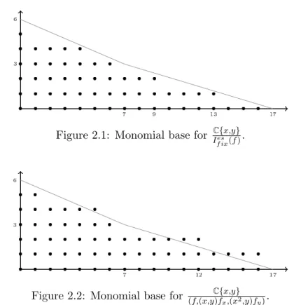
Example 1.7.1. Let '(t) = (t3_{, t}10_{), (t) = (t}3_{, t}10_,10 3 t7), (t) = (t3,103t7). The defor-mations given by • X(t, s) = t3, Y (t, s) = s1t4+ s2t5+ s3t7+ s4t8+ t10+ s5t11+ s6t14; • X(t, s) = s1t + s2t2+ t3, Y (t, s) = s3t + s4t2+ s5t4+ s6t5+ s7t7+ s8t8+ + t10+ s9t11+ s10t14; are respectively

• an equimultiple semiuniversal deformation; • a semiuniversal deformation

of '. The conormal of the deformation given by

X(t, s) = t3, Y (t, s) = s1t7+ s2t8+ t10+ s3t11;

is an equimultiple semiuniversal deformation of . The fake conormal of the deformation given by X(t, s) = s1t + s2t2+ t3, P (t, s) = s3t + s4t2+ s5t4+ s6t5+ 10 3 t 7_{+ s} 7t8;

is a semiuniversal deformation of the fake conormal of . The conormal of the deforma-tion given by X(t, s) = s1t + s2t2+ t3, Y (t, s) = ↵2t2+ ↵3t3+ ↵4t4+ ↵5t5+ ↵6t6+ + ↵7t7+ ↵8t8+ ↵9t9+ ↵10t10+ ↵11t11; with ↵2 = s1s3 2 , ↵3 = s1s4+ 2s2s3 3 , ↵4= 3s3+ 2s2s4 4 , ↵5 = 3s4+ s1s5 5 , ↵6 = 2s2s5+ s1s6 6 , ↵7= 3s5+ 2s2s6 7 , ↵8 = 10s1+ 9s6 24 , ↵9 = 3s1s7+ 20s2 27 , ↵10= 1 + s2s7 5 , ↵11= 3s7 11 , is a semiuniversal deformation of .

Example 1.7.2. Let Z = _{{(x, y) 2 C}2 _{: (y}2 _x5_)(y2 _x7_{) = 0}. Consider the}

parametrization ' of Z given by

x1(t1) = t21, y1(t1) = t51 x2(t2) = t22, y2(t2) = t72.

Let be the fake projection of the conormal of ' given by

x1(t1) = t21, p1(t1) = 5 2t 3 1 x2(t2) = t22, p2(t2) = 7 2t 5 2.

The deformations given by

• X1(t1, s) = t21, Y1(t1, s) = s1t31+ t51, X2(t2, s) = t22, Y2(t2, s) = s2t22+ s3t32+ s4t42+ s5t25+ s6t62+ t72+ + s7t82; • X1(t1, s) = s1t1+ t21, Y1(t1, s) = s3t1+ s4t31+ t51, X2(t2, s) = s2t2+ t22, Y2(t2, s) = s5t2+ s6t22+ s7t32+ s8t42+ s9t52+ s10t62+ + t7₂+ s11t82; are respectively

• an equimultiple semiuniversal deformation; • a semiuniversal deformation

of '. The conormal of the deformation given by

X1(t1, s) = t21, Y1(t1, s) = t51,

is an equimultiple semiuniversal deformation of the conormal of '. The fake conormal of the deformation given by

X1(t1, s) = s1t1+ t21, P1(t1, s) = s3t1+5 2t 3 1, X2(t2, s) = s2t2+ t22, P2(t2, s) = s4t2+ s5t22+ s6t32+ s7t42+ 7 2t 5 2+ s8t62;

is a semiuniversal deformation of the fake conormal of . The conormal of the deforma-tion given by X1(t1, s) = s1t1+ t21, Y1(t1, s) = ↵2t21+ ↵3t31+ ↵4t41+ t51, X2(t2, s) = s2t2+ t22, Y2(t2, s) = 2t22+ 3t32+ 4t42+ 5t52+ 6t62+ + 7t72+ 8t82; with ↵2= s1s3 2 , ↵3 = 2s3 3 , ↵4 = 5s1 8 , 2= s2s4 2 , 3 = 2s4+ s2s5 3 , 4 = 2s5+ s2s6 4 , 5= 2s6+ s2s7 5 , 6 = 4s7+ 7s2 12 , 7 = 1 + s2s8 7 , 8= 2s8 8 ,

is a semiuniversal deformation of the conormal of '. Example 1.7.3. Let

Z =_{{(x, y) 2 C}2: y(y4 2x5y2+ x10 4x8y x11) = 0_}.

Consider the parametrization ' of Z given by

x1(t1) = t41, y1(t1) = t101 + t111 x2(t2) = t2, y2(t2) = 0.

The deformation given by

X1(t1, s) = t41, Y1(t1, s) = t101 + t111 + s11t51+ s12t61+ s13t71+ s14t91+ s15t101 + s16t131

+ s17t141 + s18t171 + s19t181 + s20t211 + s21t251 + s22t291 ,

X2(t2, s) = t2, Y2(t2, s) = t2+ s1t2+ s2t22+ s3t32+ s4t24+ s5t52+ s6t62

+ s7t72+ s8t82+ s9t92+ s10t102 ;

is an equimultiple semiuniversal deformation of '. The conormal of the deformation given by

X1(t1, s) = t41, Y1(t1, s) = t101 + t111 + s2t91+ s3t101 + s4t131 + s5t114+ s6t171 + s7t181 ,

is an equimultiple semiuniversal deformation of the conormal of '. Let us exemplify how to get rid of

(0, 0) @ @x+ (0, t 4 2) @ @y (1.7.1)

when we go from the plane to the Legendrian case. All the other parameters that don’t figure in the Legendrian case but do so in the plane case can be eliminated proceeding

in a similar way. Let J denote the sub _OZ-module of (1.5.2) given by

m_C¯' + (x, y)˙ @ @x (x 2_{, y)} @ @y + bI. We have that xp @ @x + 1 2xp 2 @ @y 2 bI, which is equal to ✓ 10 4 t 10 1 + 11 4 t 11 1 , 0 ◆ @ @x+ 1 2 ✓ 10 4 ◆2 t16₁ + 210 4 11 4 t 17 1 + ✓ 11 4 ◆2 t18₁ , 0 ! @ @y. We have that ˙ ' = (4t3₁, 1) @ @x + (10t 9 1+ 11t101 , 0) @ @y, and 1 4(t 7 1, 0) ˙' = (t101 , 0) @ @x+ ✓ 10 4 t 16 1 + 11 4 t 17 1 , 0 ◆ @ @y,

which means that

(t10₁ , 0) @ @x+ (0, 0) @ @y = (0, 0) @ @x + ✓ 10 4 t 16 1 + 11 4 t 17 1 , 0 ◆ @ @y mod J. Similarly (t11₁ , 0) @ @x+ (0, 0) @ @y = (0, 0) @ @x + ✓ 10 4 t 17 1 + 11 4 t 18 1 , 0 ◆ @ @y mod J. As x4 _{= (t}16 1 , t42) we have that (0, 0) @ @x+ t 16 1 , 0 @ @y = (0, 0) @ @x + 0, t 4 2 @ @y mod J.

This means that, mod J, we can write (1.7.1) as a linear combination of (0, 0)_@x@ +

Chapter 2

Equisingular Deformations of

Legendrian Curves

2.1

Introduction

To consider deformations of the parametrization of a Legendrian curve is a good first approach in order to understand Legendrian curves. Unfortunately, this approach can-not be generalized to higher dimensions. On the other hand the obvious definition of deformation has its own problems. First, not all deformations of a Legendrian curve are

Legendrian. Second, flat deformations of the conormal of yk xn = 0 are all rigid, as

we recall in example 2.5.3, hence there would be too many rigid Legendrian curves. We pursue here the approach initiated in [4], following Sophus Lie original approach to contact transformations: to look at [relative] contact transformations as maps that take [deformations of] plane curves into [deformations of] plane curves. We study the category of equisingular deformations of the conormal of a plane curve Y replacing it by

an equivalent category DefYes,µ, a category of equisingular deformations of Y where the

isomorphisms do not come only from di↵eomorphisms of the plane but also from contact transformations. Here µ stands for ”microlocal”, which means ”locally” in the cotangent bundle (cf. [15], [16]).

Example 2.4.4 presents contact transformations that transform a germ of a plane

curve Y into the germ of a plane curve Y such that Y and Y are not topologically

equivalent or are topologically equivalent but not analytically equivalent.

We call equisingular deformation of a Legendrian curve to a deformation with eq-uisingular plane projection. The flatness of the plane projection is a constraint strong enough to avoid the problems related with the use of a naive definition of deformation and loose enough so that we have enough deformations.

In section 2.6 we use the results of section 2.5 on equisingular deformations of the parametrization of a Legendrian curve to show that there are semiuniversal equisingular deformations of a Legendrian curve. In particular, we show that the base space of the semiuniversal equisingular deformation is smooth. This argument does not produce a constructive proof of the existence of the semiuniversal deformation in its standard form.