SARIMA Analysis and Automated Model
Reports with BETS, an R Package
by Talitha F. Speranza, Pedro C. Ferreira, and Jonatha A. da Costa
Abstract This article aims to demonstrate how the powerful features of the R package BETS can be
applied to SARIMA time series analysis. BETS provides not only thousands of Brazilian economic time series from different institutions, but also a range of analytical tools, and educational resources. In particular, BETS is capable of generating automated model reports for any given time series. These reports rely on a single function call and are able to build three types of models (SARIMA being one of them). The functions need few inputs and output rich content. The output varies according to the inputs and usually consists of a summary of the series properties, step-by-step explanations on how the model was developed, predictions made by the model, and a file containing these predictions. This work focuses on this feature and several other BETS functions that are designed to help in modeling time series. We present them in a thorough case study: the SARIMA approach to model and forecast the Brazilian production of intermediate goods index series.
Introduction
TheBETS(Ferreira et al.,2017) package (an abbreviation for Brazilian Economic Time Series) for R (R Core Team,2017) allows easy access to the most important Brazilian economic time series and a range of powerful tools for analyzing and visualizing not only these data, but also external series. It provides a much-needed single access point to the many Brazilian series through a simple, flexible and robust interface. The package now contains more than 18,000 Brazilian economic series and contains an integrated modelling and learning environment. In addition, some functions include the option of generating explanatory outputs that encourage and help users to expand their knowledge.
BETS relies on several well-established R packages. In order to work with time series, BETS
functions build upon packages such asforecast(Hyndman,2015),mFilter(Balcilar,2016),urca(Pfaff et al.,2016) andseasonal(Sax,2016). Access to external APIs to obtain data is handled by the web scraping and HTTP tools available through thehttr(Wickham, 2017) andrvest(Wickham,2016) packages, whereas BETS own databases are queried using the packageRMySQL(Ooms et al.,2016). This article seeks to demonstrate many of these features through a practical case. We create a SARIMA model (Box and Jenkins,1970) for the Brazilian production of intermediate goods index (BPIGI) series, step by step, using mostly functions from BETS. Then, we show that BETS is capable of usingrmarkdown(Allaire,2017) to generate a fully automated report that includes a virtually identical SARIMA analysis. The report needs few inputs, runs for any given time series and has the advantage of outputting several informative comments, explaining to the user how and why it achieved the given results. The outputs, of course, vary according to the inputs. Reports provide a link to a file containing the series under analysis and the predictions calculated by the automated model. Automated reports can also produce GRNN1and exponential smoothing models, but here we focus on the previously specified methodology2. In the next section, we briefly present the SARIMA approach and show how to use BETS functions to conduct such an analysis in a typical case: predicting the future levels of the BPIGI. Then, in Section 3, we introduce the automated model reports and illustrate its capabilities by applying it to the series under study using a range of other inputs. Section 4 concludes this article.
SARIMA Analysis: A Case Study
In this section we develop a case study in which we use a handful of BETS functions to model and forecast values of the Brazilian production of intemediate goods index, following the SARIMA (Box & Jenkins) approach. Before starting the analysis we will briefly look at the methodology to be used. For a more comprehensive treatment of the topic, seeBox and Jenkins(1970) andFerreira et al.(2016)3.
1General Regression Neural Network, as proposed bySpecht(1991)
2Examples on how to use GRNN and exponential smoothing reports are available in the documentation for the functionreport().
3For a hands-on introduction, see the tutorial of Arima models offered by Duke university athttps://people. duke.edu/~rnau/411arim.htm
Box & Jenkins Methodology
The Box & Jenkins methodology allows the prediction of future values of a series based only on past and present values of the same series. These univariate models are known as SARIMA, an abbreviation for Seasonal Autoregressive Integrated Moving Average, and have the following form:
ΦP(B)φp(B)∇d∇DZt=ΘQ(B)θq(B)at, (1) where
• B is the lag operator, i.e., for all t>1, BZt=Zt−1 • P, Q, p and q are the orders of the polynomials • ΦP(B)is the seasonal autoregressive polynomial • φp(B)is the autoregressive polynomial
• ∇d= (1−B)dis the difference operator and d is the number of unit roots
• ∇D= (1−Bs)Dis the difference operator at the seasonal frequency s and D is the number of seasonal unit roots
• Ztis the series being studied
• ΘQ(B)is the seasonal moving average polynomial • θq(B)is the moving average polynomial
• atis the random error.
In its original form, which will be used here, the Box & Jenkins methodology consists of three iterative stages:
(i) Identification and selection of the models: the series is checked for stationarity and the appro-priate corrections are made for non-stationary cases, by differencing the series d times in its own frequency and D times in the seasonal frequency. The orders of the polynomials φ,Φ, θ, and Θ are identified using the autocorrelation function (ACF) and partial autocorrelation function (PACF) of the series.
(ii) Estimation of the model’s parameters using maximum likelihood or dynamic regression. (iii) Confirmation of model compliance using statistical tests.
The ACF, used in stage (i), can be defined as the correlation of a series with a lagged copy of itself as a function of lags. Formally, we can write the ACF of a time series s with realizations sifor i∈ [1, N] and mean ¯s as ACF(s, l) = ∑ N−l i=1(si−¯s)(si+l−¯s) ∑Ni=1(si−¯s)2 . (2)
Another tool for phase (i), the PACF also gives the correlation of a series with its own lagged values, but controlling for all lower lags. Let Pt,l(x)denote the projection of xtonto the space spanned by xt+1, . . . , xt+l−1. We can define the PACF as
PACF(s, l) = (
Cor(si, si+1)if l=1,
Cor(st+l−Pt,l(st+l), ... ,st−Pt,l(st))if l≥1. (3) The PACF is used to find p (the lag beyond which the PACF becomes zero is the indicated number of autoregressive terms), while the ACF is used to find q (the cut in the ACF points to the number of moving average terms). Seasonal polynomial orders, P and Q, are identified in a similar fashion, but by inspecting high values at fixed intervals. In this case, the intervals become the orders.
If the model does not pass phase (iii), the procedure starts again at step (i). Otherwise, the model is ready to be used to make forecasts. In the next section we will look at each of these stages in more detail and say more about the methodology as we go through the case study.
Some preliminary topics
The first step is to find the series in the BETS database. This can be done with the BETSsearch() function. It performs flexible searches on the metadata table that stores series characteristics. Since metadata is accessed through SQL queries, searchers are fast and the package performs well in any
environment. BETSsearch() is a crucial feature of BETS, so we provide a thorough description in this section.
Accepted parameters, expected data types, and definitions are the following:
• description - A character. A search string to look for matching series descriptions. • src - A character. The source of the data.
• periodicity - A character. The frequency with which the series is observed. • unit - A character. The unit in which the data were measured.
• code - An integer. The unique code for the series in the BETS database.
• view - A boolean. By default, TRUE. If FALSE, the results will be shown directly on the R console. • lang - A character. Search language. By default, ’pt’, for Portuguese. A search can also be
performed in English by changing the value to ’en’.
To refine the search, there are syntax rules for the parameter description:
1. To look for alternative words, separate them by blank spaces. Example: description = 'core ipca'means that the description of the series should contain the words core and ipca.
2. To search for complete expressions, put them inside single quotes (’ ’). Example: description = "index and 'core ipca'"means that the description of the series should contain the expression core ipca and the word index.
3. To exclude words from the search, insert a∼before each word. Example: description = "ipca ∼ core"means that the description of the series should contain the word ipca and should not contain the word core.
4. To exclude a whole expression from a search, place them inside single quotes (’ ’) and insert a∼before each of them. Example: description = "index ∼ 'core ipca'"means that the description of the series should contain index and should not contain core ipca.
5. It is possible to search for or exclude certain words as long as these rules are obeyed.
6. No blank space is required after the exclusion sign (∼), but it is required after each expression or word.
Finally, the command to find information about the series, which we will use throughout this article, is shown below, along with the corresponding output.
# Searching for the production of intermediate goods index series # excluding the term 'imports' from the search
results <- BETSsearch(description = "'intermediate goods' ~ imports", view = F, lang = "en") results
#> # A tibble: 3 x 7
#> code description unit periodicity start #> <chr> <chr> <chr> <chr> <chr> #> 1 11068 Intermediate go? Index M 31/0? #> 2 1334 Production indi? Index M 31/0? #> 3 21864 Physical Produc? Index M 01/0? #> # ... with 2 more variables: last_value <chr>, #> source <chr>
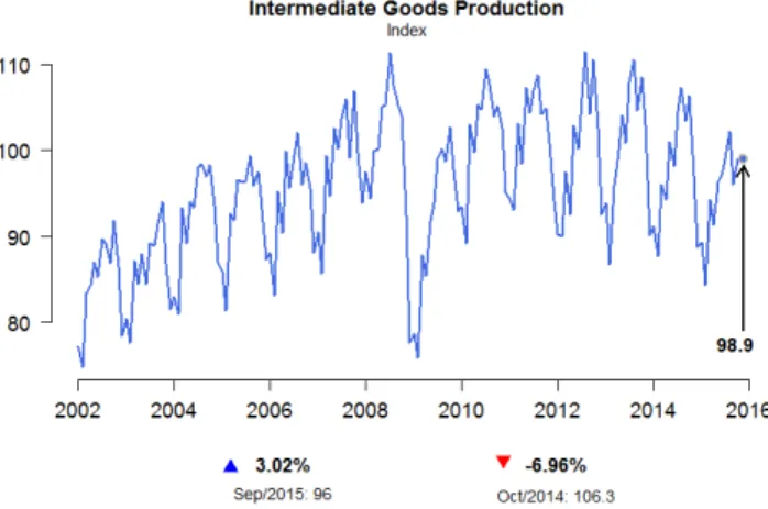
The series we are looking for is the third (code 21864). We now load it using the function BETSget() and store some values for later comparison with the model’s forecasts. We will also produce a graph (Figure1) to help formulate hypotheses about the behavior of the underlying stochastic process. The professional looking chart is created with chart(), which has the nice property of displaying useful information about the series, such as the last value and monthly/interannual variations.
# Get the series with code 21864 (BPIGI, IBGE) data <- BETSget(21864)
# Keep last values for comparison with the forecasts
data_test <- window(data, start = c(2015,11), end = c(2016,4), frequency = 12) data <- window(data, start = c(2002,1), end = c(2015,10), frequency = 12) # Graph of the series
params <- list(
title = "Intermediate Goods Production", subtitle = "Index",
colors = "royalblue")
chart(ts = data, style = "normal", open = T, params = params, file = "igp.png")
Figure 1: Graph of the BPIGI, made with function chart(). Indicators below the x coordinates
represent index variation over a month and over 12 months, respectively.
Four characteristics can be observed. First, the series is homoskedastic, with monthly seasonality. A further striking feature is the structural break in November 2008, when the international financial crisis occurred and investor confidence plummeted. This break had a direct impact on the next important characteristic of the series, the trend, which was initially clearly one of growth, albeit not at explosive rates. From November 2008 onward, however, production appeared to remain unchanged or even to fall. Since the main goal of this article is to present BETS’ features, rather than performing an overcautious time series analysis, we decided to work with fewer observations, thus avoiding problems with the structural break. Only the values from January 2009 on were used. This did not imply poorer results. In fact, discarding older values yields better predictions, at least within the SARIMA framework.
data <- window(data, start = c(2009,1), end = c(2015,10), frequency = 12)
In the following sections we create a model for the chosen series following the previously defined modelling steps.
I. Identification Stationarity Tests
This subsection covers a crucial step in the Box & Jenkins approach: checking if there are unit roots in the seasonal and non-seasonal autoregressive model polynomials and determining how many of these roots there are. If there are no unit roots, the series is stationary. In case we find unit roots, it is possible to obtain stationarity by differencing the original series. Then, the order of the polynomials can be identified using the ACF and the PACF funcitons.
The ur_test() function performs unit root tests. The user can choose among Augmented Dickey Fuller (ADF,Dickey and Fuller(1979)), Phillips-Perron (PP,Phillips and Perron(1988)), and KPSS (Kwiatkowski et al.,1992) tests. The ur_test() function was built around functions from the urca package. Relative to those, the advantage of ur_test() is the output, which is designed to quickly see the test’s results and all the needed information. The output is an object with two fields: (i) a table showing test statistics, critical values and whether the null hypothesis is rejected or not, and (ii) a vector containing the residuals of the test’s equation. This equation is shown below.
∆yt=φ1+τ1t+τ2yt−1+δ1∆yt−1+· · · +δp−1∆yt−p+1+εt (4) The test statistics in the output table refer to the coefficients φ (drift), τ1(deterministic trend) and
test parameters, ur_test() accepts the same parameters as urca’s ur.df(), as well as the desired significance level.
df <- ur_test(y = data, type = "drift", lags = 12, selectlags = "BIC", level = "5pct") # Show the result of the tests
df$results
## statistic crit.val rej.H0 ## tau2 -0.9673939 -2.89 no ## phi1 0.7526983 4.71 yes
Therefore, for the series in levels, the null hypothesis that there is a unit root cannot be rejected at a 95% confidence level, as the test statistic tau2 is greater than the critical value. We will now apply the diff function to the series repeatedly, to determine whether the differenced series has a unit root. This way we find out how many unit roots there are.
ns_roots <- 0 d_ts <- data
# Dickey-Fuller tests loop
# Execution is interrupted when the null hypothesis cannot be rejected while(df$results[1,"statistic"] > df$results[1,"crit.val"]) {
ns_roots <- ns_roots + 1 d_ts <- diff(d_ts)
df <- ur_test(y = d_ts, type = "none", lags = 12, selectlags = "BIC", level = "5pct") }
ns_roots #> [1] 1
Hence, for the series in first differences, the hypothesis that there is a unit root is rejected at the 5% significance level. We now use the nsdiffs function from the forecast package to perform the Osborn-Chui-Smith-Birchenhall test (Osborn et al.,1988) and identify unit roots at the seasonal frequency (in our case, monthly).
library(forecast)
# OCSB tests for unit roots at the seasonal frequency nsdiffs(data, test = "ocsb")
#> [1] 1
The results indicate that there is a seasonal unit root and that seasonal differencing is therefore required:
d.data <- diff(diff(data), lag = 12, differences = 1) Autocorrelation Functions
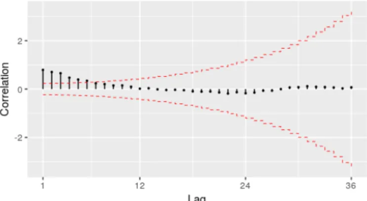
The previous conclusions are corroborated by the autocorrelation function of the series in differences (from now on,∇∇12Zt). It shows that statistically significant correlations, i.e., correlations outside the confidence interval, are not persistent for lags corresponding to multiples of 12 or values close to these multiples. This indicates the absence of a seasonal unit root.
The BETS function that we use to draw the correlograms is corrgram(). Unlike its main alternative, the forecast package’s Acf() function, corrgram() returns an attractive graph and provides the option of calculating the confidence intervals using the method proposed by Bartlett (Bartlett,1946). The greatest advantage it offers, however, cannot be shown here as it depends on Javascript. If the style parameter is set to 'plotly', an interactive graph is produced, displaying all the values of interest (autocorrelations, lags and confidence intervals) on mouse hover, as well as providing zooming, panning, and the option to save the graph in png format.
# Correlogram of differenced series
Figure 2: Autocorrelation function of∇∇12Zt
This correlogram, however, is not sufficient for us to propose a model for the series. We will therefore produce a graph of the partial autocorrelation function (PACF) of∇∇12Zt. corrgram() can also be used for this purpose.
# Partial autocorrelation function of diff(data)
corrgram(d.data, lag.max = 48, type = "partial", style="normal")
Figure 3: Partial autocorrelation function of∇∇12Zt
The ACF in Figure2and PACF in Figure3could have been generated by a SARIMA(1,0,0)(0,0,0) process. The explanation is straightforward: the ACF exhibits exponential decay and the PACF has a sharp cutoff after the first lag. This is a textbook example of an AR(1) process. Therefore, the first model proposed for Ztwill be a SARIMA(1,1,0)(0,1,0)[12] model.
II. Estimation
To estimate the coefficients of the SARIMA(1,1,0)(0,1,0)[12] model, we will use the Arima() function from the forecast package. The t tests will be performed using the t_test() function, which receives an object of type "arima" or "Arima", an integer representing the number of exogenous variables in the model and an integer for the desired significance level. It returns a data frame containing information related to the test (estimated coefficients, standard errors, test statistics, critical values and the results of the test).
# Estimation of the model parameters model1 <- Arima(data, order = c(1,1,0),
seasonal = list(order = c(0,1,0), period = 12)) # t-test with the estimated coefficients
# 1% significance level t_test(model1, alpha = 0.01)
#> Coeffs Std.Errors t Crit.Values Rej.H0 #> ar1 -0.386501 0.1099599 3.514925 2.639505 TRUE
We conclude from column Rej.H0 that the AR(1) coefficient, when estimated by maximum likeli-hood, is statistically significant at a 99% confidence level .
III. Diagnostic Tests
The aim of the diagnostic tests is to determine whether the chosen model is suitable. Here, two well-known tools will be used: analysis of standardized residuals and the Llung-Box test (Ljung and Box,1978).
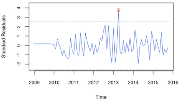
The graph of the standardized residuals will be produced with the std_resid() function, which was implemented specifically for this purpose.
# Graph of the standardized residuals resids <- std_resid(model1, alpha = 0.01) # Highlight outlier
points(2013 + 1/4, resids[52], col = "red")
Figure 4: Standard residuals from the first proposed model.
We can see that there is a prominent and statistically significant outlier in April 2013. A second model including a dummy (a time series whose values can be either 0 or 1, to control for the structural break) is therefore proposed. The dummy is defined as follows:
D1t = (
1, t=April 2013
0, otherwise (5)
This dummy can be created using the dummy() function, as shown below. The start and end parameters indicate time period covered by the dummy. The from and to fields indicate the interval within which the dummy should take a value of 1.
dummy1 <- dummy(start = c(2009,1), end = c(2015,10), year = 2013, month = 4)
Estimation of this model by maximum likelihood resulted in coefficients that are statistically different from 0 at a 1% significance level. The graph of the standardized residuals of the new model (Figure5) also shows that the decision to include Dtwas correct as there is no more evidence of a structural break.
# Estimation of the parameters of the model with a dummy model2 <- Arima(data, order = c(1,1,0),
seasonal = list(order = c(0,1,0), period = 12), xreg = dummy1) # t-test with the estimated coefficients
# 1% significance level t_test(model2, alpha = 0.01)
#> Coeffs Std.Errors t Crit.Values Rej.H0 #> ar1 -0.4063976 0.1095272 3.710472 2.639505 TRUE #> dummy 5.2072304 1.3552891 3.842155 2.639505 TRUE
resids <- std_resid(model2, alpha = 0.01) # Highlight November 2008
points(2013 + 1/4, resids[52], col = "red")
Figure 5: Standard residuals of the model proposed after the detection of a structural break
We spotted some other possible outliers in the standard residuals graph. Hence we introduce two more dummies to improve the model and then estimate a third set of coefficients.
D2t= ( 1, t=December 2012 0, otherwise (6) D3t= ( 1, t=January 2013 or February 2013 0, otherwise (7)
dummy2 <- dummy(start = c(2009,1), end = c(2015,10), year = 2012, month = 12) dummy3 <- dummy(start = c(2009,1), end = c(2015,10), year = 2013, month = c(1,2)) dummy <- cbind(dummy1,dummy2,dummy3)
model3 <- Arima(data, order = c(1,1,0),
seasonal = list(order = c(0,1,0), period = 12), xreg = dummy)
One possible way of evaluating the quality of the models is to calculate the value of an information criterion. This is already contained in the object returned by Arima().
# Show BIC for the two estimated models model1$bic
#> [1] 335.7308 model3$bic #> [1] 334.3813
Note also that the Bayesian Information Criterion (BIC,Schwarz(1978)) for the model with the dummies is smaller. Hence, based on this criterion as well, the model with the dummy should be preferred over the previous one.
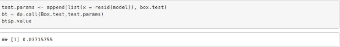
The Ljung-Box test for the chosen model can be performed with the Box.test() function in the
statspackage. We will follow Rob Hyndman’s suggestion4and use min(2m, T/5)lags, where m is the period of seasonality (12 here) and T is the length of the time series (82), which yields 16 in our case. # Ljung-Box test on the residuals of the model with a dummy
Box.test(resid(model3), type = "Ljung-Box",lag = 16) #> Box-Ljung test
#> data: resid(model2)
#> X-squared = 27.073, df = 16, #> p-value = 0.04067
The p-value of 0.041 is low and indicates there is no statistical evidence to reject the null hypothesis of no autocorrelation in the residuals. We could have added one MA term to double the p-value and generate such evidence, but we decided not to, for two reasons: (i) the law of parsimony; (ii) adding an extra term would be an ad hoc solution - we have no indication from the ACF and PACF that this term should exist; and (iii) there is no reason to be overcautious and present an extensive analysis, because our intention is to exhibit BETS’ features.
IV. Forecasts
BETS provides a convenient way of making forecasts with SARIMA, GRNN, and exponential
smooth-ing models. The predict() function receives the parameters from the forecast() function (from the package of the same name) and returns not only the objects containing the information related to the forecasts, but also produces a graph of the series including the predicted values. Displaying the information in this way is important to get a better idea of how suitable the model is. The actual values for the forecasting period can also be shown if desired.
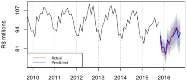
We now call predict() to generate the forecasts for the proposed model. The parameters object (object of type arima or Arima), h (forecast horizon), and xreg (the dummy for the forecasting period) are inherited from the forecast() function. The others are from predict() itself and control features of the graph, except for actual, which is the the series of effective values observed during the forecasting period.
new_dummy <- dummy(start = start(data_test), end = end(data_test)) new_dummy <- cbind(new_dummy, new_dummy, new_dummy)
preds <- predict(object = model3, xreg = new_dummy,
actual = data_test, xlim = c(2010, 2016.2), ylab = "R$ Millions",
style = "normal", legend.pos = "bottomleft")
Figure 6: Graph of the proposed SARIMA model forecasts, an output of predict
The areas in dark blue and light blue around the forecasts are the 85% and 95% confidence intervals, respectively. It appears that the forecasts were satisfactory, since in general the actual values are inside the confidence interval.
To make this statement more meaningful, we can check various measures of fit by consulting the accuracyfield contained within the predictions object (preds).
preds$accuracy
#> ME RMSE MAE MPE MAPE ACF1
#> Test set -0.08333333 2.252776 1.85 -0.2144377 2.14463 0.3403901 #> Theil's U
#> Test set 0.5675735
The other field in this object, predictions, contains the object returned by forecast() (or by another forecasting function, such as grnn.test() or predict(), depending on the model).
Using the automated report for SARIMA modeling
The report() function performs the Box & Jenkins modeling for any series chosen by the user and generates reports with the results and explanatory comments. Besides, it allows the forecasts of the model to be saved in a data file and accepts parameters in order to increase model flexibility. Each input series produce a different output, as expected. The report() prototype is as follows:
report(mode = "SARIMA", ts = 21864, parameters = NULL, report.file = NA, series.saveas = "none")
If the user changes the value of the parameter series.saveas() from ‘none’ to a valid format, the series and the model forecasts are saved in a file. series.saveas accepts all the formats save() functions can handle (namely, ‘.sas’, ‘.dta’ and ‘.spss’) plus ‘.csv’, which is very convenient. The argument ts is just as flexible, and is capable of receiving a list containing ts objects, codes of series within the BETS database, or a combination of both. A report is generated for each element on this list. For instance, the following piece of code would work:
series <- list(21863, BETSget(21864))
parameters <- list(cf.lags= 25, n.ahead = 15 ) report(ts = series, parameters = parameters)
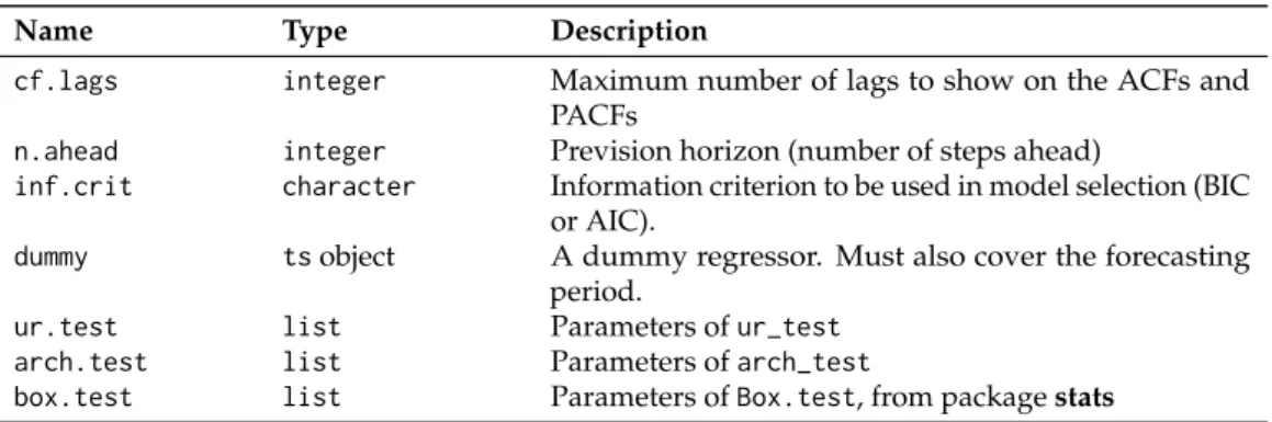
The list of reports’ specific arguments are passed through parameters, whose accepted fields vary according to the type of report (defined via mode). In the case of SARIMA models, these fields are presented in table1, all of them being optional.
Name Type Description
cf.lags integer Maximum number of lags to show on the ACFs and PACFs
n.ahead integer Prevision horizon (number of steps ahead)
inf.crit character Information criterion to be used in model selection (BIC or AIC).
dummy tsobject A dummy regressor. Must also cover the forecasting period.
ur.test list Parameters of ur_test
arch.test list Parameters of arch_test
box.test list Parameters of Box.test, from package stats
Table 1: Possible fields of parameters, an argument of report function, when mode is set to SARIMA
To model the BPIGI series in a similar way to what we modeled in the last section, we resort to the call below:
params = list( cf.lags = 48, n.ahead = 12,
box.test = list(lag = 16),
dummy = dummy(start= c(2009,1) , end = c(2016,4) , year = 2013, month = 4), ur.test = list(mode = "ADF", type = "none", lags = 12,
selectlags = "BIC", level = "5pct") )
report(ts = window(BETSget(21864), start= c(2009,1) , end = c(2015,10)), parameters = params,
series.saveas = "csv")
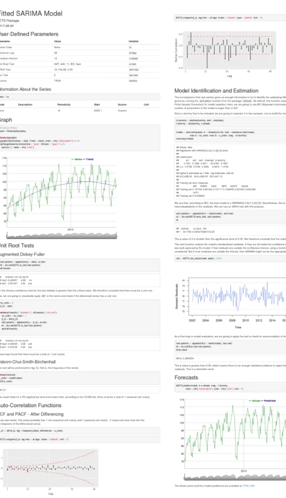
The report is rendered in the form of an html file, which opens automatically in the user’s default internet browser. This whole file is shown in Figure7. It consists of the following:
1. The information about the series as it is found in the BETS metadata table. In our example call, we use a custom series, so it exhibits more general information.
2. The graph of the series along with its trend, which is extracted with an HP Filter (Hodrick and Prescott,1997). The graph is produced with thedygraphspackage (Vanderkam et al.,2016) and enables the user to define windows and examine the series’ values.
3. The steps involved in the identification of a possible model: unit root tests (at the moment, ACF (Dickey and Fuller,1979), PP (Phillips and Perron,1988) or KPSS (Kwiatkowski et al.,1992) for non-seasonal unit roots, and OCSB (Osborn et al.,1988) test for seasonal unit roots) and correlograms of the original series (if no unit root is found), or the differenced series (if one or more unit roots are found).
4. Estimation of the parameters and display of the result from the automatic model selection performed by the auto.arima() function (from the forecast package).
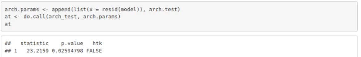
5. The ARCH test (Engle,1982) for heteroskedasticity in the residuals. If residuals are found to be heteroskedastic, the report performs a log transformation on the original series and run steps 3 and 4 again for the transformed series.
6. The graph of the standard residuals.
7. The Ljung-Box (Ljung and Box, 1978) test for autocorrelation in the residuals. If the null hypothesis of no autocorrelation is rejected, the user will be advised to use a dummy or another type of model.
8. The n-steps-ahead forecasts and a graph of the original series with the forecasted values and confidence intervals, also produced with dygraphs (this output is an option of predict()). 9. A link to the file containing the original data and the forecasts.
One example of how the output could change in response to different inputs is obtained by removing the dummy from the last example. The call without a dummy renders a report that, after detecting autocorrelation in the residuals, suggests the usage of a dummy to solve the problem (Figure 8). It does indeed solve it, as we demonstrated.
Figure 8: Snippet of the report generated without a dummy.
We now provide one more call and output snippets from the report() function, aiming at illustrat-ing its capabilities. First, suppose we need to model the Brazilian production of capital goods (BPCG) series. Its unique identifier in the BETS database is 21863, so this will be the value of parameter ts. The next piece of code builds a SARIMA report using the same dummy we needed in the case study, but ARCH test and Box test parameters are different.5
dum <- dummy(start= c(2002,1) , end = c(2017,12) , from = c(2008,7) , to = c(2008,11)) series <- window(BETSget(21863), start = c(2002,1), end = c(2017,6))
params <- list( cf.lags = 36, n.ahead = 6, dummy = dum,
arch.test = list(lags = 12, alpha = 0.03), box.test = list(type = "Box-Pierce") )
report(ts = series, parameters = params)
Figures9to11show snippets of the report that was generated by the last call and demonstrate that it presents different results when compared to the one produced previously. OCSB test, for instance, did not find any seasonal unit root, thereby displaying a different comment (Figure9).
Figure 9: First snippet of the example report with the BPCG series
In addition, residuals were found to be heteroskedastic, which forced the model to be estimated a second time, using the log transformation of the original series (Figure10).
Figure 10: Second snippet of the example report with the BPCG series
Finally, the second model was tested and considered better than the first (Figure11) and no autocorrelation in the residuals were found.
Figure 11: Third snippet of the example report with the BPCG series
Note that running a report saves a lot of time and might be insightful. However, performing the analysis in detail, using individual BETS functions rather than the batch of functions included in the reports, may provide more flexibility. Since reports use auto.arima(), they might not find models that are in line with a more sofisticated analysis. For example, the SARIMA model calculated by auto.arima() in the first example (Figure7) is not the one we proposed in the case study. This happened because the function did not find a non-seasonal unit root, since it does not test for more than 2 lags, and we tested for 6. For now, we cannot include the option of testing for more lags, the reason being that auto.arima() does not accept it.
Conclusion
We have shown in this article that the approach adopted in BETS is a novel one as it allows users not only to quickly and easily access thousands of Brazilian economic time series, but also to use and analyze these series in many different ways. Its automated reports are comprehensive, fully customizable and three methods can be readily applied: SARIMA models, GRNNs and exponential smoothing models. We showed case studies to examine the use of the first, but only mentioned the latter two. Nevertheless, the user can benefit from the extensive documentation shipped with the
package, where example code to generate GRNN and exponential smoothing reports are exhibited and discussed.
In the future we hope to expand these dynamic reports and provide new options for users. One such option has already been taken into account in the design of the package: a display mode that does not include explanations about the methodology, so that the information is provided in a more technical, succinct manner. In addition to developing new modeling methods, such as Multi-Layer Perceptrons, fuzzy logic, Box & Jenkins with transfer functions, and multivariate models, we plan to refine the analyses themselves.
Bibliography
J. J. Allaire. Rmarkdown: Dynamic Documents for R, 2017. URLhttp://cran.r-project.org/package= rmarkdown. [p133]
M. Balcilar. Mfilter: Miscellaneous Time Series Filters, 2016. URLhttp://cran.r-project.org/package= mfilter. [p133]
M. S. Bartlett. On the theoretical specification and sampling properties of autocorrelated time series. Supplement to the Journal of the Royal Statistical Society, 1946. [p137]
G. E. P. Box and G. M. Jenkins. Time Series Analysis Forecasting and Control. Holden Day, San Francisco, 1970. [p133]
G. E. P. Box and D. A. Pierce. Distribution of residual autocorrelations in autoregressive-integrated moving average time series models. Journal of the American Statistical Association, 65(332):1509–1526, 1970. [p144]
D. A. Dickey and W. A. Fuller. Distribution of the estimators for autoregressive time series with a unit root. Journal of the American Statistical Association, 74, 1979. [p136,144]
R. Engle. Autoregressive conditional heteroscedasticity with estimates of the variance of United Kingdom inflation. Econometrica, 50(4):987–1007, 1982. [p144]
P. C. Ferreira, D. Mattos, D. Almeida, I. de Oliveira, and R. Pereira. Análise De Séries Temporais Usando o R. FGV/IBRE, Rio de Janeiro, RJ, 2016. [p133]
P. C. Ferreira, T. F. Speranza, J. C. Azevedo, F. O. Teixeira, and D. Marcolino. BETS: Brazilian Economic Time Series, 2017. URLhttp://cran.r-project.org/package=BETS. [p133]
R. J. Hodrick and E. C. Prescott. Postwar U.S. business cycles: An empirical investigation. Journal of Money, Credit, and Banking, 1997. [p144]
R. J. Hyndman. Forecast: Forecasting Functions for Time Series and Linear Models, 2015. URLhttp: //cran.r-project.org/package=forecast. [p133]
D. Kwiatkowski, P. C. B. Phillips, P. Schmidt, and Y. Shin. Testing the null hypothesis of stationarity against the alternative of a unit root. Journal of Econometrics, 1992. [p136,144]
G. M. Ljung and G. E. P. Box. On a measure of a lack of fit in time series models. Biometrika, 65, 1978. [p139,144]
J. Ooms, D. James, S. DebRoy, H. Wickham, and J. Horner. RMySQL: Database Interface and MySQL Driver for R, 2016. URLhttp://cran.r-project.org/package=RMySQL. [p133]
D. R. Osborn, A. P. L. Chui, J. Smith, and C. R. Birchenhall. Seasonality and the order of integration for consumption. Oxford Bulletin of Economics and Statistics, 1988. [p137,144]
B. Pfaff, E. Zivot, and M. Stigler. Urca: Unit Root and Cointegration Tests for Time Series Data, 2016. URL http://cran.r-project.org/package=urca. [p133]
P. C. Phillips and P. Perron. Testing for a unit root in time series regression. Biometrika, 1988. [p136, 144]
R Core Team. R: A Language and Environment for Statistical Computing. R Foundation for Statistical Computing, Vienna, Austria, 2017. URLhttps://www.R-project.org/. [p133,364]
C. Sax. Seasonal: R Interface to X-13-ARIMA-SEATS, 2016. URLhttps://cran.r-project.org/web/ packages/seasonal/index.html. [p133]
G. Schwarz. Estimating the dimension of a model. The Annals of Statistics, 6, 1978. [p140]
D. F. Specht. A general regression neural network. IEEE Transactions on Neural Networks, 1991. [p133] D. Vanderkam, J. J. Allaire, J. Owen, D. Gromer, P. Shevtsov, and B. Thieurmel. Dygraphs: Interface to ’Dygraphs’ Interactive Time Series Charting Library, 2016. URLhttps://cran.r-project.org/web/ packages/dygraphs/index.html. [p144]
H. Wickham. Rvest: Easily Harvest (Scrape) Web Pages, 2016. URLhttp://cran.r-project.org/ package=rvest. [p133]
H. Wickham. Httr: Tools for Working with URLs and HTTP, 2017. URLhttp://cran.r-project.org/ package=httr. [p133]
Pedro C. Ferreira
Instituto Brasileiro de Economia (IBRE) Fundação Getúlio Vargas (FGV) pedro.guilherme@fgv.br Talitha F. Speranza
Instituto Brasileiro de Economia (IBRE) Fundação Getúlio Vargas (FGV) talitha.speranza@fgv.br Jonatha A. da Costa
Instituto Brasileiro de Economia (IBRE) Fundação Getúlio Vargas (FGV) jonatha.costa@fgv.br