Optimization of experimental design in fMRI: a general framework
using a genetic algorithm
Tor D. Wager* and Thomas E. Nichols
Department of Psychology, C/P Area, University of Michigan, 525 E. University, Ann Arbor, MI 48109-1109, USA
Received 14 February 2002; revised 1 August 2002; accepted 13 August 2002
Abstract
This article describes a method for selecting design parameters and a particular sequence of events in fMRI so as to maximize statistical power and psychological validity. Our approach uses a genetic algorithm (GA), a class of flexible search algorithms that optimize designs with respect to single or multiple measures of fitness. Two strengths of the GA framework are that (1) it operates with any sort of model, allowing for very specific parameterization of experimental conditions, including nonstandard trial types and experimentally observed scanner autocorrelation, and (2) it is flexible with respect to fitness criteria, allowing optimization over known or novel fitness measures. We describe how genetic algorithms may be applied to experimental design for fMRI, and we use the framework to explore the space of possible fMRI design parameters, with the goal of providing information about optimal design choices for several types of designs. In our simulations, we considered three fitness measures: contrast estimation efficiency, hemodynamic response estimation efficiency, and design counterbalancing. Although there are inherent trade-offs between these three fitness measures, GA optimization can produce designs that outperform random designs on all three criteria simultaneously.
© 2003 Elsevier Science (USA). All rights reserved.
Keywords:Optimization; fMRI; Genetic algorithm; Experimental design; Neuroimaging methods; Efficiency; Counterbalancing
Introduction
This article describes a method for optimizing the stim-ulus sequence in event-related fMRI using a genetic algo-rithm (GA). We describe how genetic algoalgo-rithms may be applied to experimental design for fMRI, and we present simulations of random and optimized stimulus sequences over a range of design parameters. Event-related fMRI is a major advance in methodology because of the flexibility it allows in experimental design and the specificity with which particular mental processes may be studied; but the space of possible design choices for a given study is large and com-plex, and it is difficult to know which parameter values are best. The framework for optimization we present here is general and can be used to maximize statistical and non-statistical (i.e., psychological validity) properties of fMRI designs using novel criteria or existing criteria for design
fitness (e.g., Dale, 1999; Friston et al., 1999, 2000a; Josephs and Henson, 1999; Liu et al., 2001). Previous research on optimization has considered only a narrow range of possible parameter values and design types, often excluding factors such as temporal autocorrelation of fMRI noise, nonlinear-ity in observed signal, the presence of multiple conditions and multiple contrasts of interest within a single experi-ment, experiment-related factors such as psychological probes that influence the design but are difficult to model, and factors such as counterbalancing of stimuli and repeated presentations that influence the psychological validity of the task. The flexibility of the genetic algorithm as an optimi-zation tool, combined with novel methods for estimating signal nonlinearities, allows us to circumvent all of these limitations. Within the GA framework, researchers can de-velop experimental designs that are optimal with respect to the unique characteristics of the research paradigm under investigation.
Optimization of experimental designs may best be de-scribed as a search through the space of possible designs,
* Corresponding author.
E-mail address:[email protected] (T.D. Wager).
R
Available online at www.sciencedirect.com
NeuroImage 18 (2003) 293–309 www.elsevier.com/locate/ynimg
with the dimensionality of the space defined by the number of design parameters allowed to vary. We combine use of the genetic algorithm with conventional exhaustive search over subsets of design parameters. A conventional search is used when the search space is very restricted and exhaustive search is possible. For example, when choosing an inter-stimulus interval (ISI), the search proceeds over a single-parameter dimension, and design fitness is assessed over a range of ISIs. This type of parameter mapping is feasible over a low-dimension parameter space (i.e., when trying to choose one or two design parameters). However, as Dale (1999) discovered, there is great variability among realiza-tions of random event-related designs with the same param-eter values. Optimization of the particular ordering of events is accomplished with the genetic algorithm, which is effec-tive at optimizing over very high-dimensional parameter spaces, and yields a particular pseudorandom sequence of events with maximum suitability.
Optimization of event sequences promises the greatest improvement in experimental fMRI design when rapid, event-related sequences are used. The advantages of rapid event-related fMRI over blocked fMRI or PET designs have been discussed at length (Buckner, 1998; Burock et al., 1998; Dale & Buckner, 1997; D’Esposito et al., 1999; Friston et al., 1998; Josephs and Henson, 1999; Rosen et al., 1998). Briefly, one major advantage of event-related de-signs is that they permit more specific isolation of particular psychological events than block designs, making psycho-logical inference easier and making it possible to image a whole new class of psychological events. Statistically, rapid designs (typically with ISIs⬍4 s) may improve statistical power by as much as 10:1 over single-trial designs (Dale, 1999). Not only is it possible to estimate the magnitude of regional activation using rapid designs, it is also possible to obtain reliable estimates of the time course of activation with subsecond resolution (Miezin et al., 2000).
However, all these advantages are mitigated by serious limitations posed by the shape and linearity of the signal response (e.g., BOLD) in fMRI. The statistical power of effects in rapid event-related fMRI depends greatly on the timing parameters, the particular sequence of events chosen, and how these variables interact with signal nonlinearities, temporal noise autocorrelation, and psychological factors relating to the consistency and magnitude of the expected neural activity across trials.
In this article, we first review previous approaches to experimental design optimization in fMRI. We then intro-duce the genetic algorithm and the way in which it is applied in this context. Under Methods, we describe the linear systems approach and a modification to account for nonlinearity. Following that, we describe the measures of design efficiency and the method for parameterizing an fMRI model. We then describe measures of psychological suitability (e.g., counterbalancing). Finally, we describe four simulations demonstrating the ability of the genetic
algorithm to find optimal designs for various combinations of statistical and psychological considerations.
Previous approaches to optimization of fMRI designs
Josephs and Henson (1999) were among the first to examine the relative fitness of fMRI designs in a linear system. They generated random event sequences with spec-ified transitional probabilities, performed an exhaustive search across various ISIs, and examined designs with and without temporal “jitter” or stochastic variation in event onset times (Burock et al., 1998; Dale, 1999). Their measure of fitness was “estimated measurable power” (EMP)— es-sentially the average squared deviation of a predictor from its mean.
The use of EMP as a criterion of fitness is a reasonable choice, as the statistical power of the design increases monotonically as the energy (EMP) of the predictor in-creases. However, EMP is limited because it does not take into account the other major constraint on statistical power: correlation between predictors in the design matrix.
Dale (1999) provided an alternate measure of design fitness, termed efficiency. Efficiency is the inverse of the sum of the variance of parameter estimates (see Methods, Eq. (7)). Increased variance of parameter estimates reduces the significance for a given effect size, so maximizing ef-ficiency is a reasonable endeavor. In fact, in the discipline of experimental design, maximizing efficiency leads to what are called A-optimal designs (Atkinson and Donev, 1992). The essential aspect of efficiency is that it captures col-linearity of each predictor with the others; if two predictors are nearly collinear their parameters cannot be estimated precisely. The variance of the predictor thus contains informa-tion about both the energy (EMP) of the predictor and its correlation with other predictors or combinations of predictors. If a deconvolution approach is used, as it is in Dale’s (1999) initial simulations, the efficiency reflects the power in estimating the shape of the hemodynamic response (Dale, 1999; Liu et al., 2001). If a basis set of hemodynamic response functions (HRFs) is used (Dale, 1999) or a single assumed HRF (Liu et al., 2001) is used, the efficiency statistic reflects the detection power of the design or the ability to correctly estimate the height parameter of each basis function.
However, it may often be desirable to maximize HRF shape estimation power while retaining power for contrast detection. In the extreme, contrast detection with no ability to estimate the HRF (e.g., as in a blocked design) leaves ambiguity in whether results are related to a specific psy-chological or physiological event of interest or whether they are related to other processes that occur proximally in time (Donaldson et al., 2001). For example, comparing reading of difficult words to easier words in a blocked design could lead to differences in overall level and quality of attention during difficult blocks, as well as in specific processes that occur each time a difficult word is encountered. Designs with no HRF shape estimation power confound these types of effects. Another case where HRF shape estimation is particularly useful is in estimating differences in HRF delay onset between events (Miezin et al., 2000) and in cases where the hypothesis depends on the shape of activation, as in studies that examine maintenance of information in work-ing memory over short delay intervals (Cohen et al., 1997). Friston et al. (1999) gave a formulation for the standard error of a contrast across parameter estimates for different predictors, allowing for generalization of efficiency to con-trasts among psychological conditions. It was subsequently generalized to account for temporal filtering and autocorre-lation (see Eq. (10)). This formula easily translates into a measure of the estimation efficiency of a set of contrasts (Eq. (11)), which is an important advancement because the design parameters optimal for estimating a single event type are very different from those optimal for estimating a dif-ference between two event types or another contrast across different conditions (Dale, 1999; Friston et al., 1999; Jo-sephs and Henson, 1999). Considering that most researchers in cognitive neuroscience are interested in multiple con-trasts across conditions within a single study, or at least the difference between an activation state and a baseline state, optimization strategies that take advantage of the ability to estimate efficiency for a set of contrasts are very useful.
Genetic algorithms
Genetic algorithms are a subset of a larger class of optimization algorithms, called evolutionary algorithms, which apply evolutionary principles in the search through high-dimensional problem spaces. Genetic algorithms in particular code designs or candidate solutions to a problem as a digital “chromosome”—a vector of numbers in which each number represents a dimension of the search space and the value of the number represents the value of that param-eter (Holland, 1992). Analogous with genes on a biological chromosome, the elements of a design vector in a genetic algorithm are parameters specifying how to construct an object. For example, in aircraft design, three parameters might be material, curvature of the wing foil, and wing length. Values in the design vector can be continuous, as with length, or nominal, as with material. In fMRI design, the chromosome is a vector ofNtime bins, and the values
in each slot represent the type of stimulus presented, if any, at that time. This method allows for temporal jitter at the temporal resolution of the time bins, with variable numbers of rest bins following each event of interest creating sto-chastic temporal variation (e.g., Burock et al., 1998). How-ever, the resolution specified is arbitrary.
A second common feature of genetic algorithms is that selection of designs operates on numerical measures of fitness. Design vectors must be translatable into single num-bers that represent the suitability of the design. In aircraft design, an engineer may want to minimize material costs and fuel consumption and maximize carrying capacity and maximum safe flying speed. These quantities must be as-sessed through simulation and collapsed to a single number that represents the overall suitability of a particular design specification. In fMRI, researchers may want to simulta-neously maximize the efficiency of estimation of several contrasts and the efficiency of estimating the hemodynamic response for statistical reasons and minimize stimulus pre-dictability for psychological reasons.
Three processes with analogs in evolutionary theory drive the operation of genetic algorithms: selection, cross-over, and point mutation. Genetic algorithms generally start with a population of randomly generated design vectors, test the fitness of those vectors, select the best ones, and recom-bine the parameter values (i.e., exchange some elements) of the best designs. The designs can then be tested again, and the process is iterated until some criterion is reached. This process is analogous to natural selection: Designs are ran-domly rather than explicitly constructed, but the best de-signs from each generation are carried over to the next. On average, combinations of numbers that code for desirable features tend to spread throughout the population, and the population evolves through successive generations toward higher fitness scores.
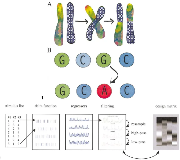
The process of exchanging elements among successful designs also has a biological analog, which is referred to as “crossover.” Although there are many ways to exchange design elements, one of the simplest is for successful (i.e., high-fitness) vectors to be paired together, as biological chromosomes are, and exchange the half of their parameters that lies above a randomly selected point along the vector. The crossover process is illustrated Fig. 1A.
A third process important in genetic algorithms is ran-dom reassignment of the values of a small number of design elements to other values, as shown in Fig. 1B. This process is analogous to point mutation in biology, which refers to the random mutation of certain components of DNA. The functional value of this process in the algorithm is to ensure that the population of designs as a whole remains hetero-geneous. Crossover relies on heterogeneity in the population; essentially, the heterogeneity determines how large of a search space the algorithm covers. While it is unlikely that random mutations alone will generate high-fitness designs, random mutation in combination with crossover can be very effective. Genetic algorithms have been applied over the past 40
years to a number of areas of science and engineering, including structural design and statistics, and recently in biology for protein folding and synthesis of proteins and drugs (Douguet et al., 2000; Sheridan et al., 2000; Yadgari et al., 1998). They are particularly suited to problems that are difficult to solve analytically or by hill-climbing techniques such as gradient descent methods used in many nonlinear fitting algorithms and expectation maximization techniques (Dempster et al., 1977). These problems typically have a large and complex “fitness landscape”—a mapping of fitness across incrementally varying parameter values, where each parameter is a dimension of the landscape. A large search space and
nonmonotonicity of fitness across many dimensions makes exhaustive search computationally prohibitive and causes hill-climbing algorithms to get stuck in local optima.
Methods
Linear systems approach
Simulation is carried out in the framework of the general linear model
Fig. 1. Illustration of crossover (A) and point mutation (B). In crossover, chromosomes in biology or vectors in a genetic algorithm pair up and exchange pieces at a randomly selected crossover point. In point mutation, certain genes or elements of a vector are randomly given a new value from the available range of possible values.
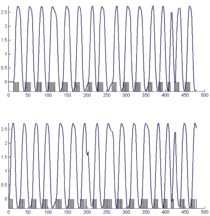
Fig. 3. Comparison of actual data for 10 subjects collected at 3 T (A) to predicted response in a linear system (B). Flickering checkerboard stimuli (120 ms) were presented, and motor responses were collected, once per second in a series of 1, 2, 5, 6, 10, or 11 stimulations, with a 30-s rest interval following the series. Data in (A) show percentages of signal change in series of each length. Linear predictions (B) were constructed by convolving a canonical HRF, normalized to the observed response height of a single checkerboard stimulation, convolved with the stimulus delta function for each series. Actual responses to long series peaked at approximately two times the height of the single stimulation response, whereas the linear convolution predicts responses over five times greater.
Fig. 4. Schematic showing the stages in GA operation. Design vectors are transformed to model matrices, which are tested for fitness. Selected designs undergo crossover, and the resulting “children” are retested iteratively until the algorithm is stopped.
Y⫽X ⫹ , (1)
whereYis thenvector of data observed at a given voxel,X
is then-by-k⫹ 1 design matrix whose columns represent the expected response,is a (k⫹1) vector of coefficients for the columns of X, and is a nvector of unobserved random errors; we make the usual assumption that eachiis
normally distributed with mean zero and variance2. There are three typical approaches to findingˆ (an estimate of). The first approach is to assume independent errors and use the usual least squares estimate,ˆ⫽(X⬘X)⫺1X⬘Y.The other two approaches, prewhitening and precoloring, account for dependent errors. LetV⫽Var()/2, the correlation matrix of the errors. Both prewhitening and precoloring estimates can be written
ˆ ⫽共共KX兲⬘KX兲⫺1共KX兲⬘KY, (2)
whereKis an-by-n(de)correlating matrix. In prewhitening,
K is chosen such thatKVK⬘is the identity matrix; in pre-coloringKis chosen such thatKVK⬘ ⬇KK⬘. The prewhit-ening approach yields the most efficient estimator ofwith colored noise, but leads to biased estimates of 2 if the estimate of the noise autocorrelation is inaccurate (Friston et al., 2000a).
The noise autocorrelation estimates used in our simula-tions were derived empirically from a visual–motor task in which subjects were asked to press the thumbs of both hands on seeing a change in a visual stimulus (Aguirre et al., 1998), which occurred every 20 s, with images acquired every 2 s over 20 trials for a total of 200 images per subject. As in previous approaches to noise estimation (Aguirre et al., 1997; Friston et al., 2000; Zarahn et al., 1997), we assumed a stationary noise model. The data were regressed on the estimated hemodynamic response and its temporal derivative, to provide a reasonably flexible model that can account for some variation in response delay, and the resid-uals were used to calculate the average cross-correlation across brain voxels for each subject, giving a 50-point estimation of the autocorrelation (Box et al., 1994), which were then averaged across seven subjects to give an auto-correlation estimate specific for our imaging environment. Although we judged this to be an adequate autocorrelation model, use of the GA framework does not depend in any way on this particular estimation method; any method judged sufficiently accurate is acceptable.
Accounting for nonlinearity
The general linear model assumes that the response to each event is independent of and sums linearly with re-sponses to other events. Several studies have demonstrated that nonlinear interactions in fMRI do occur (Birn et al., 2001; Friston et al., 2000; Janz et al., 2001; Vazquez and Noll, 1998), with the principal nonlinear effect being a saturation of fMRI signal when events are repeated less than 2 s apart. That is, the hemodynamic response to a second
event is less than to the first, and the estimated response height decreases still more for subsequent occurrences of the event. Boynton et al. (1996), although they report linear BOLD responses with respect to stimulus duration, found saturation effects in response magnitude. Other labs have found nonlinear saturation with stimulus presentation rate (Berns et al., 1999; Binder et al., 1994), consistent with the idea that closely spaced events produce signal saturation. An alternative way of conceptualizing the effect we term “saturation” is to say that the fMRI response to initial, brief events is greater than the value expected under linearity. The difference between these two conceptualizations amounts to a difference in the reference function (an im-pulse response for the saturation account and a block of stimuli for the alternative account); the same underlying phenomenon is described by both accounts. This effect is relatively small at long ISIs, but can have a substantial impact on designs with ISIs less than 4 s. Simulation with ISIs of less than 1 s may be completely untenable without a model of signal saturation. In previous simulations, design efficiency increases without bound as the ISI becomes very short (Dale, 1999; Friston et al., 1999; Josephs and Henson, 1999). In effect, discrete linear convolution, which is typi-cally used to construct predicted responses, becomes mean-ingless at short ISIs. With continuous stimulation dis-cretized at ISI s, the predicted response magnitude approaches infinity as ISI approaches zero, whereas the actual response magnitude is invariant with respect to the sampling resolution of the indicator function (i.e., the stim-ulus onset times).
In a block design with task and control periods of equal length and number of stimuli, this effect is not a problem. In continuous-stimulation block design models, where the ISI is assumed to be zero, scaling of the predictors depends on the actual sampling resolution at which the design is con-structed. This resolution is often at least equal to the repe-tition time (TR) of volume acquisitions. Sampling at differ-ent TRs results in an equivaldiffer-ent scale change in the response estimates and standard errors, leaving the resulting test statistic invariant to sampling rate. However, when block design predictors (or repeated, closely spaced events) are mixed with individual events (for an example, see Liu et al., 2001, Fig. 4), the situation becomes problematic: the scaling of the block portion of the predictor relative to the individ-ual events is arbitrary, depending on the TR, and linear convolution can yield very poor predictions of the signal response.
trains of 5, 6, 10, and 11 stimuli were approximately equal, indicating that it is difficult to increase activity above this level, as shown in Fig. 3. The peak value was about twice the magnitude of the response to a single brief impulse.
In our simulations, we modified the linear convolution by adding a “squashing function” that replaced values greater than 2⫻the impulse response with the 2⫻value. Thus, the predicted response sums linearly up to twice the impulse response height, at which it is completely saturated. While nonlinear effects are clearly more complicated than the squashing model suggests and more accurate models of nonlinearity are needed, we adopt this as an interim solution because it is easily computed and captures the basic idea of signal saturation. Again, the GA framework can accommo-date any model of nonlinear BOLD response.
Measures of design efficiency
The principal measure of uncertainty in estimation is the variance– covariance matrix of ˆ. When the data are inde-pendent, this is
Var共ˆ兲⫽2共X⬘X兲⫺1. (3)
Thus, the uncertainty in the estimates depends on the prop-erties of the design matrix and the noise variance2. When the data are dependent and (de)correlated with matrixK,we have
Var共ˆ兲⫽2共Z⬘Z兲⫺1Z⬘KVK⬘Z共Z⬘Z兲⫺1, (4)
where Z ⫽ KX, the filtered design matrix (Friston et al., 1999, 2000a). If we are interested inbcontrasts contained in ab⫻ k⫹ 1 matrixC,we focus on the variance ofCˆ.
Assuming unit variance and substituting the pseudoin-verse ofZfor (Z⬘Z)⫺1Z⬘(Graybill, 1976, p. 28), we have
Var共Cˆ兲⫽CZ⫺KVK⬘共Z⫺兲⬘C⬘. (5)
Design efficiency is the reciprocal of an arbitrary combina-tion of the diagonals of Var(Cˆ). Use of the trace corre-sponds to equally weighting each contrast of interest. We use a weighting vectorwof lengthbwhose weights repre-sent the importance of each contrast for the overall aim of the study. The overall measure of design efficiency is
⫽1/trace兵diag共w兲Var共Cˆ兲其, (6)
where diag(w) is a diagonal matrix comprised of the ele-ments ofw.Several special cases are worth considering. If
X consists of a deconvolution matrix (Glover, 1999; Hin-richs et al., 2000; Menon et al., 1998), andCis the identity
matrix, Eq. (7) gives the estimation efficiency for the shape of the HRF (Liu et al., 2001). IfCis instead replaced by a basis set of canonical HRF vectors, then the expression evaluates the efficiency of estimating the basis set (Dale, 1999). In our simulations, we useto measure efficiency of both a set of contrasts and the HRF deconvolution model for all trial types.
Parameterizing a model
The genetic algorithm works by interchanging pieces of design vectors that represent the stimulation sequence dur-ing scanndur-ing. The fitness metric, however, is derived from the filtered design matrixZassociated with the stimulation sequence. It is important, therefore, to parameterize the design matrix as accurately as possible, including data fil-tering and analysis choices (see Fig. 2).
In our parameterization of design matrices, the design vector contains one element per ISI, and the value of each element is an integer representing the stimulation condition at that time during the experiment, with 0 for rest and 1 . . .
karbitrarily assigned to conditions. For example, the integer 1 in the 5th element of the design vector might represent a visual stimulation presented at the onset of the 5th acquisi-tion, and 2 in the 10th element might represent auditory stimulation during the 10th acquisition.
Each design vector is transformed into a high-resolution design matrix whose columns are the indicator functions for the event onsets of each trial type sampled at a high time resolution (we used 100 ms) and convolved with a canonical hemodynamic response function (SPM99, http://www.fil. ion.ucl.ac.uk/spm). The design matrix is resampled at the TR, yielding the model matrixX.If a whitening approach is used, the model matrix is decorrelated as perK.If a coloring approach is used the model matrix may then be correlated via high- and/or low-pass filtering, yielding the filtered model matrix Z. Filtering is optional and depend on the projected analysis strategy for the study; in general, the simulation is most accurate when the design matrix is treated exactly like the design matrix of the actual analysis.
Psychological restriction of search space
The search through possible designs may be constrained according to a number of psychological factors, including restrictions on repetition of stimuli and transitional proba-bilities, or counterbalancing, among trial types. In the GA framework, psychological considerations are decided upon by the experimenter and implemented as either hard or soft
Fig. 5. Efficiency plots (linear model) over ISI and temporal jitter, created by inserting a number of rest intervals at random locations into the design, for Simulation 1. The length of the simulated scan was kept constant at 480 s, and the efficiency of a difference between two event types (a [1-1] contrast) was estimated for each combination of ISI and proportion of rest intervals. (A) Results assuming linear additivity of the HRF response. Efficiency approaches infinity at short ISIs because the signal response can sum without bound. (B) Line plots of efficiency as a function of ISI under the linear model for selected proportions of rest intervals, 1, 41, and 81%.
constraints. Hard constraints are implemented by excluding design vectors that do not meet specified criteria from fur-ther consideration. Soft constraints are implemented by tak-ing a weighted sum across scores on all fitness measures of interest to yield a single overall fitness score, which is then used as the criterion for selection.
Acceptable limits on stimulus repetition may vary de-pending on the psychological nature of the task. In our GA simulations, we excluded design vectors that contained more than six of the same trial type in a row anywhere in the series.
Counterbalancing of stimuli assures that the event se-quence is not predictable to participants. In a perfectly counterbalanced design, the probability of each event type is independent of the event history. For counterbalancing to the first order, we consider the joint probability of trial type
jfollowing trial typei,which is
pij⫽pipj, (7)
whereiandjindex trial type, from 1 tok,andpiandpjare the base rates for each trial type. If all events occur at equal rates, thenpij⫽1/k2, and in a counterbalanced design each event type follows each other one equally often. The ex-pected number of trials of typejfollowing typeiis
E共Nij兲⫽apij, (8)
whereais the number of stimulus presentations. In matrix notation,
E共N兲⫽app⬘, (9)
wherep⫽{p1. . .pk} is a column vector of base rates. The formula can be generalized to counterbalancing up to therth order. In anrth order counterbalanced design, we consider the joint probability of trial type j on the current trial and trial typeiat lagr, E(Nijr). Thus the overall expected values given an rth order counterbalanced design can be repre-sented by ak⫻k⫻rthree-way arrayE(N). In practice, the expected number of stimulus presentations per condition at each time lag r is the same, so E(N..r) contains the same values for allr.
Given the expected number of trials for each combina-tion of stimulus presentacombina-tion orders, it is simple to compute the deviation of any design vector from perfect counterbal-ancing. Thek⫻k⫻rarrayN,which represents the number of observed occurrences of event pairi, jwith time lagr,is compared to the expected arrayE(N) by taking the average sum of squared differences between the two arrays. This yields an overall counterbalancing score f with a lower bound of 0 indicating perfect counterbalancing. The asso-ciated fitness measure ⫽ 1 ⫺ f (so that higher values signify greater fitness) can be used to compare design vec-tors with one another and can be computed using
⫽1⫺ 1
IJR
冘
ijr共Nijr⫺E共Nijr兲兲2 (10)
While designs with large have good overall counterbal-ancing, we are also concerned with the worst-case counter-balancing for any given trial type. Hence we may impose a hard constraint by eliminating any designs for which max 兵共Nijr ⫺ E共Nijr兲兲2其exceeds 10% of the expected number of stimuliE(Nijr).
We also need to constrain the degree to which a design vector contains the desired frequencies of each trial type. This quantification is necessary because the recombination of design vectors in the GA does not strictly maintain the input frequencies for all design vectors. We define
⫽1⫺max兩g⫺ab兩, (11)
where g is a k-length vector containing the number of observed events in each condition.
Search methods: exhaustive search and genetic algorithm
As the optimization of trial structure is a search through parameter space, the search algorithm used should depend on the size and complexity of the search space and the fitness landscape or the mapping of design fitness onto search parameters. Small search spaces can be mapped using exhaustive search, in which every combination of parameters (or a set covering the space with reasonable thoroughness) is tested, and the ultimate design is selected by using the design with the highest estimated fitness. As an example, we chose to estimate the optimal ISI and temporal jitter (introduced by inserting a random number of rest intervals into an event-related design; Burock et al., 1998) by generating random designs at a range of simulations and testing their fitness using the detection power measure de-scribed above. The results of these tests are reported in Simulation 1.
We used the GA to choose the optimal ordering given a selected ISI and number of rest intervals. The starting point for the GA was a population of design vectors created with the desired number of events in each condition in random order. Design matrices were constructed for each design vector, and fitness measures to be limited by hard constraint (including , , and maximum number of re-peated events, depending on the simulation) were estimated for each.
Each fitness measure was standardized by the population mean and standard deviation; this makes the metrics com-parable and gives more weight to measures with small variability. A linear combination of these standardized mea-sures that defines the overall fitness measure
F⫽w˜⫹w˜⫹w˜, (12)
where˜,˜, and˜ are the standardized efficiency, counter-balancing, and condition frequency measures, respectively, andw,w, and ware their weights.
(cho-sen arbitrarily to implement a soft cutoff in fitness scores) and combined with a uniform(0,1) variate:
Ft⫽rand关0,1兴⫹1/共1⫹e⫺
␣F兲
, (13)
where Ft is the transformed fitness score, and ␣ is a constant representing selection pressure or the degree of “softness” in the selection process. Design vectors with
Ftabove the median were selected for crossover. “Selec-tion pressure” in this context is the probability of select-ing a design with F ⬍ F. The case ␣ ⫽ 0 produces random selection (allFtare equal), and␣3⬁produces a step function where all designs with above-median Ft
also have above-median F. The best value for ␣ was determined to be 2.1, found by systematically varying the parameter value and observing the GA’s performance; specifically, the GA produced designs of highest fitness per iteration in our simulations with this value of␣. Use of random noise with the sigmoid transform allowed for some random variation in which designs were selected, preserving population variability. This principle of pro-moting diversity is important for systems that rely on natural or stochastic variation to produce optimal de-signs, and we found it to be helpful here.
Selected design vectors are paired at random and crossed over at a single randomly selected point until the population limit is reached. The portion of the vectors that lies above the crossover point is exchanged, so that the new design vectors consist of pieces of two “parent” vectors. After crossover, as in biology, a small percentage (we chose 0.1%) of the values across all lists are subject to random mutation, in which two vector elements are randomly inter-changed. This process can provide additional leverage for selection, but its main function is to maintain variability in the population and prevent the system from getting “stuck” in a suboptimal solution.
Another concern is the population becoming too homogeneous. So another step taken is to introduce randomness if all lists are too correlated. Specifically, if the average correlation between lists rises above 0.6, 10% of the event codes of each design are replaced with random event codes. The event codes to be replaced are randomly selected for each design, and the best design is left intact.
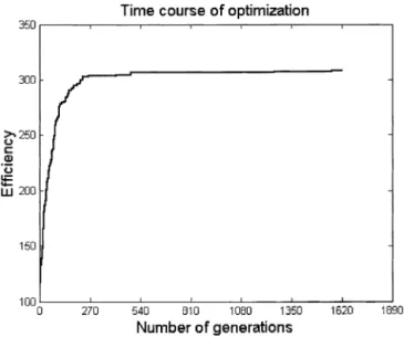
To preserve the integrity of the most optimal design thus far, a separate copy is made of this design and inserted into the population without crossover or mutation. The popula-tion of new design vectors is then reevaluated for fitness, and the process of evaluation, selection, and crossover con-tinues iteratively until a specified number of generations is reached, as shown in Fig. 4. An alternate strategy to using a fixed number of generations is to monitor convergence by plottingFt(e.g., see Fig. 9) and exiting the algorithm when the system does not improve in a specified number of generations.
Simulations
Simulation 1
This simulation demonstrates exhaustive search over ISIs and jitter. This simulation was designed to maximize detection efficiency for a [1⫺1] contrast across two equally probable conditions and generate an efficiency surface ex-ploring the ISI by trial density space. No filtering was used, andVdetermined from local data was used for this and all other simulations, except where otherwise noted. The effi-ciency of 100 random event sequences at each combination of ISI and jitter was estimated, and their mean efficiency was used as the population reference. ISI ranged from 0.1 to 16 s, in increments of 0.1, and jitter ranged from 1% of the total stimulation periods being rest intervals to 81% rest intervals. The TR was 2 s, with 240 acquisitions; these parameters were used for all simulations. Separate simula-tions were run with and without nonlinear saturation.
Simulation 2
Previous researchers have suggested that block designs are more efficient at detecting differences between condi-tions than event-related ones (Dale, 1999). This simulation examines this assertion by using the GA to optimize the efficiency for a [1⫺1] contrast across two equally probable conditions with no intrinsic autocorrelation model (i.e., in-dependent noise), no filtering, and no psychological con-straints. In this situation, the GA should converge on a block design. We explored this prediction further by rerunning the simulation with a highly autocorrelated noise model. The noise model was created with the autocorrelation func-tion 1/(t/14 ⫹ 1), where t is time in seconds, chosen to resemble typical highly autocorrelated data from our scan-ner (see Fig. 8C). We reasoned that increased scanscan-ner noise at low frequencies should push the optimal design into higher frequencies so that it overlaps less with the noise. For both of these simulations, TR and ISI were fixed at 2 s and no nonlinear saturation was used. Generation size was 500.
Simulation 3
This simulation was designed to test the ability of the GA to optimize multiple efficiency measures simultaneously and to compare GA optimization versus random search through design space. The GA was set to optimize detection efficiency for a single predictor, with half of the events being the condition of interest and half being rest. The TR was 2 s and the ISI was 2 s. An identical simulation was performed using random search instead of the GA. Rather than subjecting design vectors to crossover, the random search algorithm simply rerandomized the event order in the population of design vectors and tested their fitness, saving the best vector at each iteration. The algorithm returned the best single design vector tested. Both simulations were run for equal time, each examining approximately 13,000 de-signs (45 generations for the GA). Generation size was 300.
In a second set of simulations, we used random and GA search algorithms, with the same parameters, to optimize both contrast and HRF estimation efficiency simulta-neously. If there is latitude to partially circumvent the in-herent trade-off between contrast estimation and HRF esti-mation, the GA may produce designs that are superior to randomized designs on both efficiency measures.
Simulation 4
The purpose of this simulation was to test the ability of the GA to simultaneously optimize multiple constraints across a range of ISIs for more than two conditions. We simulated rapid event-related designs with four condi-tions at an ISI of 1 s and compared the performance of the
GA after 1128 generations of 300 event lists each (10 h of optimization) with groups of 1000 random designs at ISIs ranging from 0.4 to 8 s. The GA optimized (1) efficiency for a [1 1-1-1] contrast across the trial types, (2) HRF estimation efficiency across the trial types, (3) counterbalancing of all trial types up to third order, (4) 1 and 2, or (5) 1–3. Rest periods were included and main-taining the input frequencies of each condition was not specified as a priority (w⫽ 0), so the GA could select the number of rest periods in the optimal design; the average time between trials of each type could vary, with a lower limit of ⬃ 4 s. This constraint was implicit in construction of the simulation with 1 s ISI and four trial types of interest.
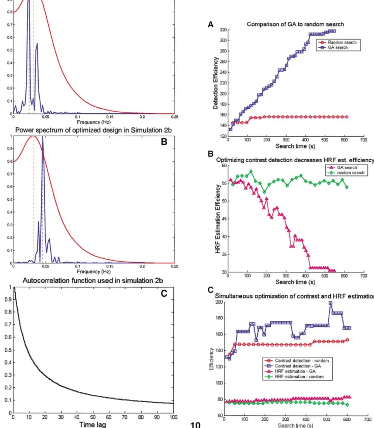
Fig. 8. (A) Spectral density plots of the optimized model (blue line) and the canonical SPM99 HRF (red line). (B) The same spectral profiles for a optimized model assuming high noise autocorrelation, with the autocorrelation function shown in (C). The frequency of block alternations in the evolved model increases under high noise autocorrelation, moving the power spectrum of the signal out of the range of the noise.
Computation times
Several metrics might be used to measure gains in effi-ciency using GA or other search algorithms. One might choose to track efficiency as a function of number of cycles (generations), number of models tested, or computation time. We present simulations here in terms of computation time, annotated with description of the number of cycles. Although computation time depends on the speed of the computer system, for a given system, run time is the most direct way to compare different search parameters and al-gorithms, and how much time it takes to achieve a certain result is in some sense the “bottom line” in choosing a way to search. The number of models tested and the number of cycles depend on the particulars of the simulation and are not comparable across different simulations even on the same computer.
For comparability, all simulations were run on a Pentium III 700-MHz computer with 128 Mb of RAM. In 10 min of search time with a generation size of 300 designs, the GA could complete approximately 45 cycles totaling⬃13,000 designs tested. These numbers also depend on the length of the designs and the complexity of the filtering and autocor-relation options, but where we compare simulation times, these variables are held constant.
Results and discussion
Simulation 1
The surface maps in Figs. 5 and 6 show efficiency as a function of ISI and trial density assuming signal response linearity (Fig. 5A and B) and assuming a simple nonlinear
squashing of the signal response at 2⫻the impulse response (Fig. 6A and B). Results assuming linearity essentially rep-licate the findings of Josephs and Henson (1999, Fig. 2). Efficiency increases exponentially as ISI approaches zero, with dramatic increases at ISIs of less than 0.7 s. This result occurs because the signal is allowed to sum linearly without bound, and at short ISIs the signal magnitude approaches infinity.
Simulation assuming nonlinear saturation provides more reasonable estimates, although the nonlinearity model is only a rough approximation. With no rest periods, these results suggest that an optimal ISI is around 2.2 s, giving an average time between trials of the same type of 4.4 s. In this case, the random ordering of the trials provides the neces-sary temporal jitter, and additional rest intervals decrease power. However, at short ISIs (2 s or less), it becomes advantageous to insert rest intervals (Fig. 6), as the signal begins to saturate at these ISIs.
With greater degrees of nonlinearity, the optimal ISI grows longer. In a parallel simulation (not shown), we found that using a saturation value of 1.6⫻ resulted in an optimal ISI of 3 s or an average of 6 s between trials of the same type. Accurate models of signal nonlinearity will allow researchers to make better estimates of optimal pa-rameter choices.
These results are for detecting differences between two conditions. If the goal is to estimate the shape of the hemo-dynamic response, or detect other contrasts, a different efficiency surface would be expected. The strength of this approach is that one can generate an efficiency surface specific to the aims and design requirements of a particular study, taking into account a specific autocorrelation model, filtering options, contrasts of interest, psychological design constraints, and estimation strategy. Once a particular combination of parameters is chosen from the efficiency surface, the GA can be used to further optimize the particular trial ordering.
Simulation 2
Results show that as expected, the GA converged on a block design (Fig. 7) and that the peak of the power spec-trum closely matched the peak of the power specspec-trum of the HRF (Fig. 8A). The peak power of the optimized design was at 0.025 Hz or 40.0 s periodicity, slightly lower in frequency than the HRF, with a second peak just above the peak frequency of the HRF. The peak power of the HRF occurred at 0.032 Hz or 31.5 s periodicity. With a high-autocorrelation noise model (Fig. 8C), corresponding to the increased low-frequency drift, we found that the solution of the GA was a block design with a higher frequency of alternation. Fig. 8B shows that the power spectrum for the design peaks at mod: 0.046 Hz, 21.8 s periodicity, substan-tially higher in frequency than the HRF power peak. Based on these results, the optimal design for detecting a differ-ence between two conditions depends on the noise autocor-relation in the scanner. In particular, higher autocorautocor-relation
calls for higher-frequency designs. As Fig. 9 shows, the GA converged on the block design in approximately 250 gen-erations.
Simulation 3
Fig. 10A shows detection efficiency over the search time for the GA and the random search algorithm. The GA produced much greater gains in efficiency with more itera-tions, indicating that it outperformed the random search algorithm. The random search algorithm was also somewhat effective; the range of efficiency for 1000 random designs was 63.05 to 142.37, with the best design substantially less efficient than produced by either GA search. However, as shown in Fig. 10B, optimizing detection efficiency comes at an inherent cost in HRF estimation efficiency, as predicted by Liu et al. (2001). In the GA simulation, HRF estimation efficiency is below the range of HRF estimation efficiency scores for random designs (efficiency ranges from 44.54 to 58.50 for 1000 random designs), indicating that the gains in contrast estimation power with the GA optimization came at the cost of decreases in HRF estimation efficiency.
An important additional question is whether the GA could optimize both detection efficiency and HRF estima-tion efficiency simultaneously. The results of a simulaestima-tion
using both GA and random search methods are shown in Fig. 10C. With GA search, contrast efficiency improves substantially within 2 min (less than 10 generations), and the HRF estimation efficiency improves somewhat more slowly. The GA substantially outperforms random search on both measures. These results indicate that it is possible to achieve a reasonable balance between detection and HRF estimation ability. Although the optimized design is much more efficient than random event permutations on both measures, it is inferior to optimizing a single measure.
Simulation 4
The purpose of this simulation was to test the ability of the GA to simultaneously optimize multiple constraints (˜,
˜, and˜ ) at a range of input ISIs. In Fig. 11, we express the results of both random simulations at a range of ISIs and the optimized designs in terms of fitness as a function of the average time between repeated events of the same type.
The results show that a short ISI—1 s, with ⬃ 4 s between same-type events—produces the best contrast ef-ficiency in random designs, with a slightly longer optimal time between repetitions (⬃6 s) for HRF estimation effi-ciency. The results suggest that a compromise at ⬃5 s between trials of the same type will produce the best
simul-Fig. 11. Simulation 4: Optimized and block designs (black dots) compared to the mean of 1000 random sequences (black lines) on three fitness measures: (A) contrast detection efficiency (eff), (B) HRF estimation efficiency (hrf), and (C) counterbalancing (cbal). 95% confidence intervals for individual random designs at each value on the abscissa are indicated by dashed black lines. Optimizing for a particular fitness measure produces significant costs in other fitness measures. Optimizing for multiple measures produced designs that were well above random designs on all optimized measures, but not as good as is possible with selective optimization.
taneous optimization of contrast and HRF efficiency, as indicated by the line peaks in Fig. 11A (contrast efficency) and Fig. 10B (HRF efficiency), at a small cost in counter-balancing (Fig. 11C). These results are in good agreement with similar models from other simulations (e.g., Birn et al., 2002, Fig. 2). Simultaneous optimization of contrast and HRF efficiency produced a design that was substantially better than random designs on both measures, as shown in Table 1, but was inferior to single-criterion optimization, 1:2.00 for contrast and 1:1.33 for HRF estimation. Optimi-zation of all three fitness criteria still produced a design that was better than random designs on all three measures (Fig. 11, Table 1). This result indicates that although there are trade-offs between measures of fitness, those trade-offs are not absolute. The importance of any of the fitness criteria depends on the particular goals of the study.
Extensions of the GA framework
One advantage of the GA framework is that it allows for estimation of design fitness with any arbitrary design. Ex-perimenters are not limited to modeling simple one-or two-condition designs; the choice of autocorrelation models, HRF types, and design types is arbitrary. In our lab, we have used the GA framework to develop and test mixed block/ event-related designs, designs in which the stimulation is an extended epoch rather than a brief event, designs in which the conditions of interest involve dependencies among trials (e.g., task switching experiments, in which the events of interest involve changes between processing different types of stimuli, rather than the occurrence of any particular stimulus), self-paced designs, and experiments with probe and instruction periods inserted into the stimulus sequence, which change the spectral characteristics of the design. Although the possibilities are nearly limitless, the principle remains the same throughout these modifications:
parame-terize your model, choose relevant fitness measures, and let the GA find an exceptional model.
Conclusions
Based on our simulations, it appears that it is difficult to simultaneously optimize the ability to detect a response, the ability to estimate the shape of the response, and counter-balance the ordering of events in a stimulus sequence. How-ever, GA optimization produces designs that are much more effective by all of these criteria than random ordering of the event sequence. In addition, the GA framework produces more effective results than random search through the space of possible event orderings.
For our assumed model of the HRF and signal nonlin-earity, these simulations suggest that the optimal design for detecting main effects or differences is a block design with 21– 40 s periodicity, depending on the amount of noise autocorrelation, which produced approximately a 6:1 power advantage over randomized event-related designs in our simulations of difference detection across four conditions [A⫹ B ⫺ (C⫹ D)]. Given no other constraints, the GA framework rapidly converges to this design. For random designs, the best choice of ISI for both contrast detection and HRF estimation is one that produces trials of the same condition that are an average of 5 s apart (i.e., a 2.5-s ISI with two trial types or a 1.25-s ISI with four trial types). As nonlinear saturation of the signal response increases, the optimal ISI increases as well. Temporal jitter is recom-mended if the design involves only a single event type, if only main effects are of interest, or if the ISI is less than 2 s (for two-condition designs). However, use of an optimized, pseudorandom trial order can improve on random designs even at the optimal ISI.
Optimization of fMRI trial design is a difficult problem, with a number of considerations that depend jointly on the characteristics of fMRI signals, the characteristics of the brain response elicited, and the psychological goals of the study. Because of the great variation in types of design and study goals, it is difficult to come up with a simple set of rules that will produce the optimal design in all situations. The GA takes a step toward solving this problem by allow-ing researchers to specify designs with great flexibility, potentially capturing many of the idiosyncrasies of a study and optimizing the statistical and nonstatistical properties of the design with respect to the particular concerns of the study.
Acknowledgments
Thank you to Doug Noll, Rick Riolo, John Jonides, Ed Smith, Rick Bryck, Steve Lacey, and Ching-Yune Sylvester for helpful discussions on this material. This work was supported in part by a National Science Foundation
Grad-Table 1
Ratio (%) of efficiencies for selected designs compared to random designsa
Optimization type Fitness measure
Contrast eff. HRF est. Counterbalancing
Block design 657 13 95.7
Contrast efficiency 577 70 96.5
HRF estimation eff. 80 136 99.2
Counterbalancing 107 79 102.2
Contrast⫹HRF 289 120 99.5
Contrast⫹HRF⫹ counterbalancing
217 119 101.2
aPercentage scores are calculated as the fitness of the optimized (or
uate Research Fellowship to T.D.W. and by a National Institute of Mental Health grant to John Jonides.
References
Aguirre, G.K., Zarahn, E., D’Esposito, M., 1997. Empirical analyses of BOLD fMRI statistics. II. Spatially smoothed data collected under null-hypothesis and experimental conditions. NeuroImage 5 (3), 199 – 212.
Aguirre, G.K., Zarahn, E., D’Esposito, M., 1998. The variability of human, BOLD hemodynamic responses. NeuroImage 8 (4), 360 –369. Atkinson, G.L., Donev, A.N., 1992. Optimum Experimental Designs.
Clar-endon Press, Oxford.
Berns, G.S., Song, A.W., Mao, H., 1999. Continuous functional magnetic resonance imaging reveals dynamic nonlinearities of “dose-response” curves for finger opposition. J. Neurosci 19 (14), RC17.
Binder, J.R., Rao, S.M., Hammeke, T.A., Frost, J.A., Bandettini, P.A., Hyde, J.S., 1994. Effects of stimulus rate on signal response during functional magnetic resonance imaging of auditory cortex. Brain Res. Cogn. Brain Res 2 (1), 31–38.
Birn, R.M., Cox, R.W., Bandettini, P.A., 2002. Detection versus estimation in event-related fMRI: choosing the optimal stimulus timing. Neuro-Image 15 (1), 252–264.
Birn, R.M., Saad, Z.S., Bandettini, P.A., 2001. Spatial heterogeneity of the nonlinear dynamics in the fmri bold response. NeuroImage 14 (4), 817– 826.
Boynton, G.M., Engel, S.A., Glover, G.H., Heeger, D.J., 1996. Linear systems analysis of functional magnetic resonance imaging in human VI. J. Neurosci 16 (13), 4207– 4221.
Box, G.E.P., Jenkins, G.M., Reinsel, G.C., 1994. Time Series Analysis: Forecasting and Control, third ed. Prentice Hall, Englewood Cliffs, NJ. Buckner, R.L., 1998. Event-related fMRI and the hemodynamic response.
Hum. Brain Mapp 6 (5– 6), 373–377.
Burock, M.A., Buckner, R.L., Woldorff, M.G., Rosen, B.R., Dale, A.M., 1998. Randomized event-related experimental designs allow for ex-tremely rapid presentation rates using functional MRI. NeuroReport 9 (16), 3735–3739.
Cohen, J.D., Perlstein, W.M., Brower, T.S., Nystrom, L.E., Noll, D.C., Jonides, J., Smith, E.E., 1997. Temporal dynamics of brain activation during a working memory task. Nature 386 (6225), 604 – 608. Dale, A.M., 1998. Optimal experimental design for event-related fMRI.
Hum. Brain Mapp 8 (2–3), 109 –114.
Dale, A.M., Buckner, R.L., 1997. Selective averaging of rapidly presented individual trials using fMRI. Hum. Brain Mapp 5, 329 –340. Dempster, A.P., Laird, N.M., Rubin, D.B., 1977. Maximum likelihood
from incomplete data via the EM algorithm. J.R. Stat. Soc. Ser. B Method. 39, 1–22.
D’Esposito, M., Zarahn, E., Aguirre, G.K., 1999. Event-related functional MRI: implications for cognitive psychology. Psychol. Bull. 125 (1), 155–164.
Donaldson, D.I., Petersen, S.E., Ollinger, J.M., Buckner, R.L., 2001. Dis-sociating state and item components of recognition memory using fMRI. NeuroImage 13 (1), 129 –142.
Douguet, D., Thoreau, E., Grassy, G., 2000. A genetic algorithm for the automated generation of small organic molecules: drug design using an evolutionary algorithm. J. Comput. Aid. Mol. Des. 14 (5), 449 – 466. Friston, K.J., Josephs, O., Rees, G., Turner, R., 1998. Nonlinear
event-related responses in fMRI. Magn. Reson. Med. 39 (1), 41–52. Friston, K.J., Josephs, O., Zarahn, E., Holmes, A.P., Rouquette, S., Poline,
J., 2000a. To smooth or not to smooth? Bias and efficiency in fMRI time-series analysis. NeuroImage 12 (2), 196 –208.
Friston, K.J., Mechelli, A., Turner, R., Price, C.J., 2000b. Nonlinear re-sponses in fMRI: the Balloon model, Volterra kernels, and other he-modynamics. NeuroImage 12 (4), 466 – 477.
Friston, K.J., Zarahn, E., Josephs, O., Henson, R.N., Dale, A.M., 1999. Stochastic designs in event-related fMRI. NeuroImage 10 (5), 607– 619.
Glover, G.H., 1999. Deconvolution of Impulse response in event-related BOLD fMRI. NeuroImage 9, 416 – 429.
Graybill, F.A., 1976. Theory and Application of the Linear Model. Dux-bury Press, Belmont, CA.
Hinrichs, H., Scholz, M., Tempelmann, C., Woldorff, M.G., Dale, A.M., Heinze, H.J., 2000. Deconvolution of event-related fMRI responses in fast-rate experimental designs: tracking amplitude variations. J. Cogn. Neurosci. 2 (Suppl 2), 76 – 89.
Holland, J.H., 1992. Genetic algorithms. Sci. Am. 267 (1), 66 –72. Janz, C., Heinrich, S.P., Kornmayer, J., Bach, M., Hennig, J., 2001.
Coupling of neural activity and BOLD fMRI response: new insights by combination of fMRI and VEP experiments in transition from single events to continuous stimulation. Magn. Reson. Med. 46 (3), 482– 486. Josephs, O., Henson, R.N., 1999. Event-related functional magnetic reso-nance imaging: modelling, inference and optimization. Phil. Trans. R. Soc. Lond. B Biol. Sci. 354 (1387), 1215–1228.
Liu, T.T., Frank, L.R., Wong, E.C., Buxton, R.B., 2001. Detection power, estimation efficiency, and predictability in event-related fMRI. Neuro-Image 13 (4), 759 –773.
Menon, R.S., Luknowski, D.C., Gati, J.S., 1998. Mental chronometry using latency-resolved functional MRI. Proc. Natl. Acad. Sci. USA 95, 10902–10907.
Miezin, F.M., Maccotta, L., Ollinger, J.M., Petersen, S.E., Buckner, R.L., 2000. Characterizing the hemodynamic response: effects of presenta-tion rate, sampling procedure, and the possibility of ordering brain activity based on relative timing. NeuroImage 11 (6 Pt 1), 735–759. Rosen, B.R., Buckner, R.L., Dale, A.M., 1998. Event-related functional
MRI: past, present, and future. Proc. Natl. Acad. Sci. USA 95 (3), 773–780.
Sheridan, R.P., SanFeliciano, S.G., Kearsley, S.K., 2000. Designing tar-geted libraries with genetic algorithms. J. Mol. Graph. Model. 18 (4 –5), 320 –334 525.
Vazquez, A.L., Noll, D.C., 1998. Nonlinear aspects of the BOLD response in functional MRI. NeuroImage 7 (2), 108 –118.
Yadgari, J., Amir, A., Unger, R., 1998. Genetic algorithms for protein threading. Proc. Int. Conf. Intell. Syst. Mol. Biol. 6, 193–202. Zarahn, E., Aguirre, G.K., D’Esposito, M., 1997. Empirical analyses of
BOLD fMRI statistics. I. Spatially unsmoothed data collected under null-hypothesis conditions. NeuroImage 5 (3), 179 –197.