A NON-STANDARD OPTIMAL CONTROL PROBLEM ARISING IN AN ECONOMICS APPLICATION
Alan Zinober* and Suliadi Sufahani
Received May 3, 2012 / Accepted July 10, 2012
ABSTRACT.A recent optimal control problem in the area of economics has mathematical properties that do not fall into the standard optimal control problem formulation. In our problem the state value at the final time the state,y(T)=z, is free and unknown, and additionally the Lagrangian integrand in the functional is a piecewise constant function of the unknown valuey(T). This is not a standard optimal control problem and cannot be solved using Pontryagin’s Minimum Principle with the standard boundary conditions at the final time. In the standard problem a free final statey(T)yields a necessary boundary conditionp(T)=0, wherep(t)is the costate. Because the integrand is a function ofy(T), the new necessary condition is that
y(T)should be equal to a certain integral that is a continuous function ofy(T). We introduce a continuous approximation of the piecewise constant integrand function by using a hyperbolic tangent approach and solve an example using a C++ shooting algorithm with Newton iteration for solving the Two Point Boundary Value Problem (TPBVP). The minimising free value y(T) is calculated in an outer loop iteration using the Golden Section or Brent algorithm. Comparative nonlinear programming (NP) discrete-time results are also presented.
Keywords: optimal control, non-standard optimal control, piecewise constant integrand, economics, com-parative nonlinear programming results.
1 INTRODUCTION
Calculus of Variations (CoV) provides the mathematical theory to solve extremizing functional problems for which a given functional has a stationary value either minimum or maximum [13]. Optimal control is an extension of CoV and it is a mathematical optimization method for deriving optimal control policies. Optimal control channels the paths of the control variables to optimize the cost functional whilst satisfying (in this paper) ordinary differential equations. Economics is a source of interesting applications of the theory of CoV and optimal control [7]. A few classical examples that reflect the use of optimal control are the drug bust strategy, optimal production, optimal control in discrete mechanics, policy arrangement and the royalty payment problem [5, 7, 9].
*Corresponding author
In a recently studied economics problem a firm struggling with intensively low demand of their product will purposely increase the marginal cost by reducing the production of the product and increase the selling price [11]. Therefore the requirement to pay a flat-rate royalty on sale has the effect of increasing the marginal cost and thereby decreasing the output while simultaneously increasing the price. The effect of permitting a nonlinear royalty leads to a non-standard CoV problem not previously considered. In this paper we will demonstrate some ways of solving the problem without discussing the precise economics details.
Let us start by considering a simple problem. We wish to determine the control functionu(t)
wheret ∈ [0,T]that maximises the integral functional
J[(·)] = Z T
0
f(t,y(t),u(t),y(T))dt (1)
subject to satisfying the state ordinary differential equation d ydt = u(t)with y(0)known and the endpoint state valuey(T)at timet=T unknown. The Lagrangian integrand depends on the unknown final valuey(T)and this is not a standard optimal control problem because the function depends ony(T). A standard optimal control often solves a problem with the final state y(T)
free and then the boundary condition p(T)is zero [12]. The Hamiltonian for optimal control theory arises when using Pontryagin’s Minimum Principle (PMP) [13]. It is used to find the optimal control for taking a dynamical system from one state to another subject to satisfying the underlying ordinary differential equations [12]. We introduce a continuous approximation of the piecewise constant integrand function by using a hyperbolic tangent approach. The present paper will indicate how such problems can be solved. In the next section we will discuss the theoretical approach in order to solve the problem. We will follow the work of Malinowska and Torres [6], in proving the boundary condition for CoV [2]. Then we will demonstrate a numerical example and we will use C++ to solve it. We also compare the results with a nonlinear programming(NP) discrete-time approach and then present some conclusions.
2 NON-STANDARD OPTIMAL CONTROL
In classical optimal control problems, the function (1) does not depend specifically on the free value y(T). However, in our case, the Lagrangian integrand function f depends on y(T). We present a recent theorem that indicates that p(T)is equal to a certain integral at time T. Ma-linowska and Torres [6] have proven this boundary condition for CoV on time scales [2]. The following theorem can be applied to our problem.
Theorem:[6, 7]
Ify˜(·)is the solution of the following problem
J[(·)] = Z T
0
f t,y(t),y˙(t),y(T)dt (2)
y(·)∈C1 (4)
then
d
dt fy˙ t,y˜(t),y˙˜(t),y˜(T)
= fy t,y˜(t),y˙˜(t),y˜(T)
(5)
for allt∈ [0,T]. Moreover
fy˙ t,y˜(t),y˙˜(t),y˜(T)= −
Z T
0
fz t,y˜(t),y˙˜(t),y˜(T)dt
From an optimal control perspective one [12, 13] has the costatep(T)= fy˙ t,y˜(t),y˙˜(t),y˜(T).
Hence
p(T)= − Z T
0
fz t,y˜(t),y˙˜(t),y˜(T)dt (6)
wherep(t)is the Hamiltonian multiplier or costate function. Theorem 1 shows that the necessary optimal condition does not havep(T)=0 as is the case for the standard classical optimal control problem.
Suppose that we wish to consider a piecewise constant function f in (2). For example, consider
J[(·)] =
Z T
0
f(t,y(t),u(t),z)dt
wherez=y(T)and
f(t,y,u,z)=0.3u(t)2+W(zy(t)sin(πt)+0.5) (7)
and
W = (
a for y≤0.5z
b for y>0.5z (8)
witha andbreal numbers. We have a discontinuous integrand that cannot be differentiated as required in the final boundary condition (7). We introduce a continuous approximation of the piecewise constant integrand function by using a hyperbolic tangent approach in order to have a continuous smooth function. Other approximations have been tried but they required hundreds of terms, for instance in a Fourier series approximation. The tanh(ky)approximation used here is very accurate. A numerical example will be presented in the next section.
3 NUMERICAL EXAMPLE
The example is a simplified version of the proposed economics problems but has the same main features. The state equation (ODE system) is described by
˙
y(t)=u(t) (9)
We wish to maximise
J[(·)] = Z T
0
where
f(t,y,u,z)=3
4
√
u−W(y)
19
20 +zysin
π
t 10
u(t)
(11)
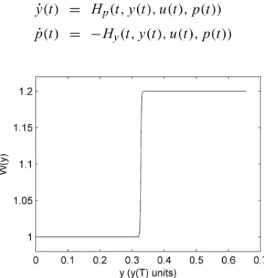
is a continuous function andT =10.W(y)is a piecewise constant function where
W(y)=
(
1 for y≤0.5z
1.2 for y>0.5z (12)
We approximateW(y)using a hyperbolic tangent function
W =1.1+0.1 tanh(k(y−0.5)) (13)
and we select k suitably large. k = 450 say. For larger values of k we obtain a smoother approximation of the functionW(y)(see Fig. 1). The known initial state is y(0)=0 and final state valuez=y(T)is free. Therefore the Hamiltonian is described byH(t,y,u,p)= f+p.u and
˙
y(t) = Hp(t,y(t),u(t),p(t)) (14)
˙
p(t) = −Hy(t,y(t),u(t),p(t)) (15)
Figure 1–W(y)approximation.
The costate satisfies
˙
p=40−40 tanh(50y−25z)2
19
20+zysin
π
t 10
u(t)+W zsin π t 10
u(t) (16)
The stationarity condition isHu=0 and this yields
u(t)= 9
64W1920+zysin π10t −p2
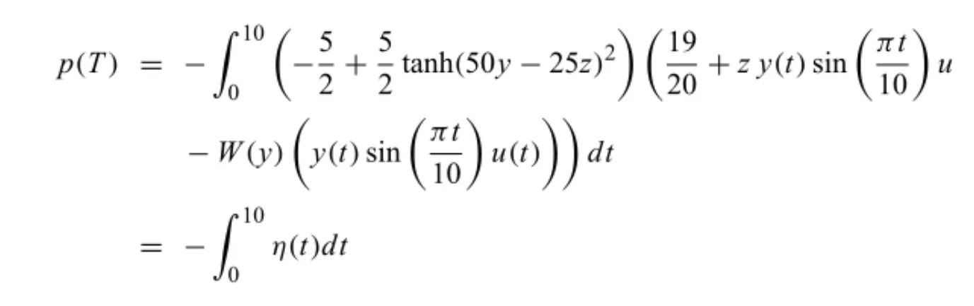
Equation (6) holds so
p(T) = − Z 10
0
−5
2+ 5
2tanh(50y−25z)
2 19
20+z y(t)sin
π
t 10
u
−W(y)
y(t)sin
π
t 10
u(t)
dt
= − Z 10
0
η(t)dt
4 RESULTS
There are several necessary conditions that need to be satisfied, such as the state equation (9) and the costate equation (16) along with the stationarity condition (17). Also the initial condition of y(0)is given and we select a guessed initial value of p(0). We also need to make sure the boundary condition of (18) will be satisfied at the final time,T. This is a two point boundary value problem. We need to ensure that the iteration value ofzused in (17) will be equal toy(T)
at the final timeT. This is satisfied in our algorithm only when the p(T)boundary condition converges. Then we will have the optimal solution. The minimising free valuey(T)is calculated in an outer loop iteration using the Golden Section (or Brent) maximising line search algorithm. We used the Newton shooting method with two guessed valuesv1 = p(0)andv2= p(T). We use the programming language C++ in order to solve the shooting method and other algorithms described in the Numerical Receipe library [8]. We iterate the system with the state equation y(t), costate equationp(t), the integral ofη(t)and the cost function J(t).
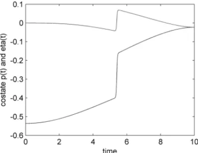
An optimal solution was obtained with high accuracy. The results are
y(T)=0.654221, p(T)= −0.022793, eta(T)= −0.022793 and J(T)=1.138440.
Figures 2–4 shows the optimal curves of the state variable y(t), adjoint variable p(t)and the integraleta(t)and the control variableu(t).
Figure 3– Costate v time shooting algorithm.
Figure 4– Control v time shooting algorithm.
As a comparative approach, we used a different nonlinear programming discrete-time technique to solve the same problem [1, 7]. We solved the problem using Euler and also Runge-Kutta discretisation, and an optimization algorithm in order to solve the unknown control variablesuk
at each timetk [1]. We used the AMPL program language [3] and the MINOS nonlinear solver
with 45 time steps in order to solve the problem.
reset;
#################### ### PARAMETERS ### param N = 45; param x0 = 0; param T = 10; param N1 = N-1; param TN = T/N; param S = T/N/2;
### VARIABLES ### var x {0..N}, default x0; var u {0..N} >= 0.0001; ################### ### OBJECTIVE ###
maximize J: sum {j in 0..N1} (0.75*sqrt(u[j]) - (1.1+0.1*tanh(450.0*x[j]25.00*x[N]))*0.95*u[j]
-(1.1+0.1*tanh(450.0*x[j]-225.00*x[N]))*x[N]*x[j]*u[j]*sin(pi*j*TN/10))*TN; #####################
### CONSTRAINTS ###
subject to xinit: x[0] = x0 ; ### RK4 METHOD
var xp1 {i in 0..N1} = u[i];
var xp2 {i in 0..N1} = u[i] + S*xp1[i]; var xp3 {i in 0..N1} = u[i] + S*xp2[i]; var xp4 {i in 0..N1} = u[i] + TN*xp3[i];
subject to xdyn {i in 0..N1}: x[i+1] = x[i] + TN*(1/6*u[i] + 2/3*(u[i]+u[i+1])*0.5 + 1/6*u[i+1]);
subject to uN : u[N] = u[N1];
############# SOLVING OPTIONS ############## option solver minos;
solve;
###### OUTPUT SCREEN display J;
display x[N]; display xinit;
printf: " # N = %d\n", N; printf: " # Data\n";
printf{i in 0..N-1}: " %24.16e %24.16e %24.16e %24.16e\n\n", i*TN, x[i], u[i], xdyn[i];
printf: " %24.16e %24.16e %24.16e\n", J, x[N], u[N-1];
display {i in 0..N1} i*TN, x, xdyn, u > resultzurichRK.txt; end;
Figures 5–7 show the plot of optimal results for both the shooting and nonlinear programming (NP) approaches for the state variable y(t), costate and control variableu(t). The results are essentially the same. The NP results are good but the Hamiltonian shooting approach is a much more accurate approach.
5 CONCLUSION
Figure 5– State v time shooting and NP(x) algorithms.
Figure 6– State v time shooting and NP(x) algorithms.
REFERENCES
[1] BETTSJT. 2001. Practical methods for optimal control using nonlinear, Advances in Design and Control, Society for Industrial and Applied Mathematics (SIAM), Philadelphia, PA.
[2] FERREIRARAC & TORRESDFM. 2008. Higher-order calculus of variations on time scales. Math-ematical control theory and finance, pp. 149–159. Springer, Berlin.
[3] FOURERR, GAYDM & KERNIGHANBW. 2002. AMPL: a modelling language for mathematical programming, Duxbury, Press/Brooks/Cole Publishing Company.
[4] STEFANI G. 2009. Hamiltonian approach to optimality conditions in control theory and nons-mooth analysis. Nonsnons-mooth analysis control theory and differential equations, INDAM, Roma. http://events.math.unipd.it/nactde09/sites/default/files/stefani.pdf.
[5] LEONARD D & LONG NV. 1992. Optimal control theory and static optimization in economics, Cambridge University Press, Cambridge.
[6] MALINOWSKA AB & TORRES DFM. 2010. Natural boundary conditions in the calculus of variations. Mathematical Methods in the Applied Sciences, 33(14): 1712–1722. Wiley, doi: 10.1002/mma.1289.
[7] PEDROAFC, TORRESDFM & ZINOBERASI. 2010. A non-classical class of variational problems with application in economics. International Journal of Mathematical Modelling and Numerical Optimisation,1(3): 227–236. InderScience, doi: 10.1504/IJMMNO.2010.031750.
[8] PRESSWH, TEUKOLSKYSA, VETTERLINGWT & FLANNERYBP. 2007. Numerical recipes: The art of scientific computing. Third edition. Cambridge Univ. Press, Cambridge.
[9] SETHISP & THOMPSONGL. 2000. Optimal control theory – Applications on management science and economics. Second edition. Kluwer Academic Publishers, Boston, MA.
[10] VINTERR. 2000. System and control: foundation and application optimal control, Birkha Boston, Springer-Verlag New York, New York.
[11] ZINOBERASI & KAIVANTOK. 2008. Optimal production subject to piecewise continuous royalty payment obligations, internal report.
[12] KIRKDE. 1970. Optimal control theory: An introduction. Prentice-Hall Network Series, New Jersey.