ORIGINAL PAPER
Back to the edge: relative coordinate system for use-wear analysis
Ivan Calandra1 &Lisa Schunk1,2&Alice Rodriguez3&Walter Gneisinger1&Antonella Pedergnana1&Eduardo Paixao1,4& Telmo Pereira4&Radu Iovita3,5&Joao Marreiros1,2,4
Received: 8 November 2018 / Accepted: 28 January 2019 # The Author(s) 2019
Abstract
Use-wear studies rely heavily on experiments and reference collections to infer the function of archeological artifacts. Sequential experiments, in particular, are necessary to understand how use-wear develops. Consequently, it is crucial to analyze the same location on the tool’s surface during the course of an experiment. Being able to relocate the area of interest on a sample is also essential for reproducibility in use-wear studies. However, visual relocation has limited applicability and there is currently no easy and efficient alternative. Here we propose a simple protocol to create a coordinate system directly on the sample. Three ceramic beads that serve as reference markers are adhered onto the sample, either with epoxy resin or acrylic polymer. The former is easier to work with but the latter is reversible so it can be applied to archeological samples too. The microscope’s software then relocates the position(s) of interest. We demonstrate the feasibility of this approach and measure its repeatability by imaging the same position on an experimental flint blade 10 times with two confocal microscopes. Our results show that the position can be relocated automatically with a horizontal positional repeatability of approximately 14% of the field of view. Quantitative surface texture measurements according to ISO 25178 vary due to this positional inaccuracy, but it is still unknown whether this variation would mask functional differences. Although still perfectible, we argue that this protocol represents an important step toward repeatability and reproducibility in experimental archeology, especially in use-wear studies.
Keywords Confocal microscopy . ISO 25178 . Lithics . Repeatability . Surface texture . Traceology
Introduction
Experimental archeology has become one of the most impor-tant tools in Paleolithic archeology. In use-wear studies in particular, experiments are necessary to build up reference collections to which the archeological samples are compared. Yet, most studies have focused only on the wear produced after the experiment, while neglecting the state before use in
the experiment (e.g., Bofill et al.2013; Portillo et al. 2013; Stemp et al. 2015; Sano and Oba 2015; Key et al.2015; Watson and Gleason 2016; Galimova and Sitdikov 2017; Queffelec et al. 2018). However, no surface is perfectly smooth, meaning that the topography already present before the experiment (i.e., surface topography due to tool manufacturing orBunused^ topography) has an effect on the development of wear. To tackle this problem, some studies
Electronic supplementary material The online version of this article (https://doi.org/10.1007/s12520-019-00801-y) contains supplementary material, which is available to authorized users.
* Ivan Calandra [email protected]
1
TraCEr, Laboratory for Traceology and Controlled Experiments at MONREPOS Archaeological Research Centre and Museum for Human Behavioural Evolution, RGZM, Neuwied, Germany
2 Institute for Prehistoric and Protohistoric Archaeology, Johannes
Gutenberg University, Mainz, Germany
3 Anthrotopography Laboratory, Center for the Study of Human
Origins, Department of Anthropology, New York University, New York City, NY, USA
4
ICArEHB, Interdisciplinary Center for Archaeology and Evolution Human Behaviour, University of Algarve, Faro, Portugal
5
Early Prehistory and Quaternary Ecology, University of Tübingen, Tübingen, Germany
have analyzed nearby unused areas (e.g., Stemp et al.2013,
2018) or unused experimental samples (e.g., Stemp and Stemp
2001, 2003; Evans and Donahue 2005, 2008; Evans and Macdonald2011; Macdonald 2014; Werner2018) that are assumed to show the same unused topography. However, no two surfaces are identical: even two surfaces from the same sample will have different unused topographies. This differ-ence becomes fundamental when quantitative 3D use-wear analyses are applied. Other studies (e.g., Asryan et al.2014; Ollé and Vergès2014; Evans et al.2014; Pedergnana et al.
2016; Chabot et al.2017; Benito-Calvo et al.2018; Martisius et al.2018) have therefore analyzed how use-wear develops through sequential experiments, in which the researchers tried to visually relocate the same surface before, during, and after the experiment. However, this approach only works if the surface has not changed to the point that it is not recognizable anymore (Martisius et al.2018). Moreover, it is highly depen-dent on the scale of analysis, where smaller areas are harder to find again visually than larger ones. This is true, for example, when using scanning electron (SEM) or confocal microscopes at high magnifications. In summary, there is a need to auto-matically relocate the area of interest without visual compar-isons (Martisius et al.2018). To our knowledge, only Stemp and Stemp (2003) and Martisius et al. (2018) developed such a system by scratching the sample to create a reference point on the sample.
Here we present a simple protocol to automatically relocate a position on a sample, either before, during, and after an experiment, or for the re-analysis of samples with different microscopes/analyses (e.g., archeological samples, samples stored in reference collections). The method described here can work with any type of microscope featuring a motorized stage and associated software. In order to quantify the poten-tial of the method to affect the measurement of surface topog-raphy, we applied it with confocal microscopes. While we tested this method only on experimental samples, it can also be applied to archeological samples.
The goals of the present study were to (1) demonstrate the coordinate system functionality on two confocal microscopes from different manufacturers, (2) measure the X-Y positional repeatability of the coordinate system functionality on each microscope, and (3) measure the variability in surface topog-raphy due to this positional (in)accuracy. We were therefore not interested in comparing the positional repeatability of each microscope. We argue that, whatever the repeatability of the microscope and associated software used is, the coordinate system functionality available to the user should be applied because it is in any case better than finding the location man-ually and visman-ually.
Hereafter, following Leach (2013), the term surface topography will be used to describe the overall surface structure, while surface form is defined as the shape of the object, and surface texture is what remains when the
form is removed from the topography. These definitions differ from Evans et al. (2014), where texture describes the roughness and topography the waviness (both includ-ed in Leach’s (2013) texture), the distinction between roughness and waviness being based on wavelength filters (see below).
Materials and methods
Samples
We selected two experimental tools displaying use-wear. Both tools (FLT1-4 and FLT1-7) are blades knapped from flint from the French Pyrenees (Narbonne-Sigean Basin). They were used in mechanical bi-directional linear (cutting-like) action on dry wood (Pinus sp.) boards. Each blade performed 250 strokes of 2 × 30 cm at 0.5 m.s−1with a 4.5 kg load applied onto the tool (Pereira et al. in prep.).
Ceramic beads were adhered onto the ventral side of the samples to be used as reference points for the defini-tion of a coordinate system directly on the samples. For this, epoxy resin was used on sample FLT1-7. Epoxy resin is, in the strict meaning of the term, not reversible and should not be applied to archeological samples. Therefore, Paraloid B72, an acrylic polymer used routinely in archeological conservation, was also tested and applied to sample FLT1-4. Paraloid B72 is easily reversible (i.e., dissolved) with acetone or ethyl acetate. The sample FLT1-4 was used to demonstrate the applicability of Paraloid B72 (see below for details); it was not used for further analysis, as the aim was to show the feasibility of the procedure using a conservation grade adhesive. It should be remembered that the specific glass transition temperature (Tg) of an adhesive might cause the adhesive to flow, if placed under a localized heat source such as microscope lighting other than LED.
Cleaning procedure
The samples were placed in new individual plastic bags filled with ~ 300 mL of demineralized water and a nonionic deter-gent (BASF Plurafac LF901, 1 g/L = 1% w/v; BASF SE, Ludwigshafen, Germany). They were then immersed into an ultrasonic bath (EMAG Emmi 20HC) pre-heated at 40 °C and left for 5–10 min to reach the bath temperature. Ultrasonic action was applied for 15 min at 45 KHz and 150 W.
Subsequently, samples were rinsed in two steps: (1) the bags were filled and emptied 3 times with tap water to remove surfactant residues and (2) the bags were filled with ~ 300 mL demineralized water and immersed into the 40 °C bath for 5–10 min and another 15 min of ultra-sonic action at 45 KHz and 150 W to remove residues
from all previous steps. Finally, the samples were covered and left to air-dry overnight.
The measured area (around the edge) was cleaned again with 2-propanol 70% v/v and lens cleaning tissues just before acquisition.
Beads
Ceramic beads were adhered to the ventral side of the samples either with epoxy resin (FLT1-7) or Paraloid B72 (FLT1-4) (see Online Resource1).
The epoxy resin component (Epoxydharz L) was mixed with the hardener component (Härter S) in a 10:4 ratio by weight. Black pigment concentrate (Universal-Farbpaste, Schwarz), maximum 2% weight, was added to make the p r e p a r a t i o n m o r e v i s i b l e . T h i x o t r o p i c f i l l e r (Thixotropiermittel) was also added on demand to reduce viscosity. All components are manufactured by R&G Faserverbundwerkstoffe GmbH (Waldenbruch, Germany). The pot life of the entire preparation is up to 1.5 h, and the curing time is approximately 24 h. Resin drops were applied via a needle-point onto the flint surface under a Leica M420 stereo-microscope at low magnification (× 120–× 180). After about 30 min, 100–200 μm diameter ceramic beads (SiLiBead Type ZY-S 0,1-0,2; Sigmund Lindner GmbH, Warmensteinach, Germany) were applied via a needle-point wetted with 2-propanol, although we realized later that the residual resin was enough for the needle-point to remain sticky to handle the beads without alcohol (see Online Resource 1). This 30 min delay was necessary to ensure that the beads would not sink into the resin pool. The beads were centered as precisely as possible in the resin pool.
Paraloid B72, an EA/MMA copolymer, was dissolved in ethyl acetate (Kremer Pigmente GmbH & Co. KG, Aichstetten, Germany) to 25% w/w. The dissolved polymer starts to set by evaporation of solvent more or less instanta-neously. Polymer drops were applied via a needle-point onto the flint surface under a binocular. Ceramic beads were ap-plied via a needle-point wetted with ethyl acetate.
In both cases, the beads were adhered approximately in the same plane as the region of interest, several millime-ters away from the active parts of the tool (e.g., edge). This ensures that the beads would not be removed during the experiments. Additionally, epoxy resin and ceramics are strong and resilient materials that should offer suffi-cient resistance to accidental displacement. The beads were adhered 5–10 mm apart; they should not be placed in a straight line but no specific angle between the beads is required (Fig.1). While decreasing the size of the beads might offer processual advantages, they become increas-ingly challenging to manipulate.
3D data acquisition
Scanning conditions
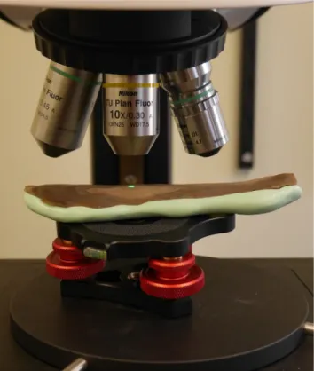
A mold was taken of the dorsal side of the flint blade (FLT1-7) to ensure that the sample will stay stable during acquisition (Fig.2). Indeed, plasticine (Patafix) was found to be too soft so that the sample was moving a few mi-crometers per minute, which was enough to be detected and to influence the acquisition. Moreover, plasticine can be difficult to remove from (archeological) samples, which can compromise future residue analysis (e.g., Pedergnana et al. 2016). The mold was made of Provil n o v o P u t t y r e g u l a r s e t ( K u l z e r G m b H , H a n a u , Germany), a two-component silicone impression material comprising base paste and matching catalyst paste for addition curing that hardens in 3–5 min at ambient room conditions.
The sample was positioned with the measured area as horizontal as possible (Fig.2) to minimize the vertical (z-axis) measuring range. For this, the sample had to be tilted slightly. The tilt required is dependent on the mor-phology of the sample and on the area of interest on the sample. Temperature and humidity were measured con-stantly in both labs.
Confocal microscopes and acquisition settings
We acquired 3D surface topography data on sample FLT1-7 with two confocal microscopes, also called opti-cal profilometers: (1) an upright light microscope Axio Imager.Z2 Vario coupled to a laser-scanning confocal mi-croscope (LSCM) LSM 800 MAT (Carl Zeiss Microscopy GmbH) at the laboratory for Traceology and Controlled Experiments (TraCEr) at MONREPOS, Germany, and (2) a Sensofar S neox optical profilometer (Sensofar Metrology, Barcelona, Spain) at the Anthrotopography Laboratory at New York University, USA. They are here-after referred to as BLSM^ and BS neox^, respectively. Other confocal microscopes may feature a similar func-tionality, and, if so, could also be used; for example, the Olympus LEXT or the Leica DCM8 (identical to the S neox, except for the objectives).
All relevant information and settings are listed in Table 1. Both systems were turned on at least 1 h before starting acquisition, so that all components were warmed up to limit thermic drift during acquisition. The coordi-nate system was created and calibrated (see section BCoordinate system^ below) with 10× objectives, while
the 3D surface topography was acquired with 50× objec-tives. The fields of view are fixed for each microscope and objective combination. With the 50× objectives, the fields of view measure 255.56 × 255.56 μm on the LSM
and 350.88 × 264.19 μm on the S neox (Table 1). The frame size is fixed on the S neox (1360 × 1024 pixels) but it can be adjusted with up to 6144 × 6144 pixels on the LSM. Frame size was therefore set to 991 × 991 pixels on the LSM in order for the pixel size (or measuring point spacing = field of view/frame size) to be identical on both microscopes: 0.258μm in X and Y directions.
Coordinate system
Zeiss’s ZEN blue (for the LSM) and Sensofar’s SensoSCAN (for the S neox) software packages can achieve the same goal: automatically find a location on a sample again and again. Three markers on the sample are needed for both systems. These markers serve as reference points to define a coordinate Fig. 1 Overview of the two samples prepared for this study, FLT1-4 (a-b)
and FLT1-7 (c-d). Photos of the tools (a, c) and close-ups of the attached beads (b, d) on each sample, rotated 90° counter clockwise relative to the overview photos. The numbering of the beads corresponds to the order of the reference markers. Photos were taken with a Nikon DSLR camera
D610 with a Nikon AF-S VR Micro-Nikkor 105 mm f/2.8G IF-ED lens. Close-ups were acquired with a Smartzoom 5 equipped with a PlanApo 1.6×/0.1 objective at × 34 total on-screen (17.5″) magnification (Carl Zeiss Microscopy GmbH)
system directly on the sample (see Online Resource2for step-by-step instructions on each microscope’s software).
Acquisition was performed on each microscope by ap-plying the following procedure. (1) The coordinate system was created before the first scan, using the three adhered beads as reference points with the 10× objective. (2) One area with visible polish was located and scanned with the 50× objective. (3) The sample was removed from the mi-croscope stage and lifted from its molded support. (4) The sample was repositioned on the stage with its orientation (rotation and tilt) as close as possible to the original ori-entation. (5) The coordinate system was then calibrated again with the 10× objective and the microscope software automatically moved the microscope XY stage so that the same location was positioned under the objective. (6) This location was scanned again with the 50× objective, with-out further manual adjustments of the stage. Deviations from scan to scan therefore only result from pre-positioning (rotation and tilt) errors, positional reproduc-ibility of the stage motors, and inaccuracy (rounding) of the software calculations. (7) The process was repeated so that the sample was scanned 10 times with each microscope.
Since the coordinate systems cannot be exchanged from one microscope and software package to the other, we had to create and use two different coordinate systems, one for
each microscope. However, we tried to manually find the lo-cation of the first scan on the first microscope (LSM) for the first scan on the second microscope (S neox), so that the ac-quired surfaces are as similar as possible. Therefore, the first scan on each microscope was located manually; the subse-quent nine scans were located automatically with the software packages. This is not critical because, as stated above, the goal is not to compare the two pieces of equipment.
3D data processing
The resulting 3D surface data were processed in ConfoMap v7.4.8633 (a derivative of MountainsMap Imaging Topography developed by Digital Surf, Besançon, France). A template was applied to each 3D surface (n = 20) with the following procedure: (1) extract the topographic layer, (2) extract the 255.56 × 255.56μm area (991 × 991 pixels) from the top left corner, (3) apply a Gaussian low-pass S-filter (S1 nesting index = 0.425μm, end effects managed) to remove noise and keep the primary surface, (4) apply an F operator (polynomial of degree 3) to remove the form and keep the SF surface, i.e., texture, (5) apply a Gaussian high-pass L-filter (L nesting index = 127μm, end effects managed) to filter out the waviness and keep the SL surface, i.e., roughness, and (6) threshold the surface between 0.010 and 99.9% material ratio to remove the aberrant positive and negative spikes. Steps 1–2 were applied to surfaces from the S neox only. See Online Resource3for details and for results on each surface.
This template follows Digital Surf’s Metrology Guide (ac-cessible at https://guide.digitalsurf.com/en/guide.html) and therefore the ISO 25178 norm (International Organization for Standardization2012) as closely as possible, but it should not be expected that lithic tool surfaces require the exact same processing as dictated by the ISO norms, defined for industrial applications. Moreover, such surfaces constrain some process-ing settprocess-ings. We therefore adapted the cutoff values for the filters based on field of view as follows: The L nesting index cannot be larger than half the shortest side (breadth) of the field of view, i.e., 255.56/2 = 127.78μm, truncated to 127 μm. The ISO 4287/4288 norms (International Organization for Standardization1996,1997) state thatλs(2D equivalent of the S1nesting index) should be 300 times smaller than λc (2D equivalent of the L nesting index), i.e., 0.426μm, rounded to 0.425μm. These norms also recommend the pixel size to be no larger than one-fifth ofλs/S1, i.e., 0.0852μm, which would result in 255.56/0.0852 = 3000 pixels in X and in Y directions on the LSM, or 350.88/0.0852 = 4119 pixels in X and 264.19/ 0.0852 = 3111 pixels in Y on the S neox. The detector of the LSM can measure up to 6144 × 6144 pixels, but the CCD camera sensor of the S neox is limited to 1360 × 1024 pixels. So pixel size was limited to 0.258μm in both X and Y direc-tions, as explained above.
Fig. 2 View of the sample FLT1-7 during definition of the coordinate system with the S neox: a manual goniometer is used to orientate the region of interest as horizontally as possible and a silicon mold holds the sample in place. The same setup was used on the LSM
Much more work is needed to define the best way to analyze the surfaces of archeological tools but this task is beyond the scope of the present study. The processing workflow was performed consistently to enable the com-parison, which was the goal. It is not intended as a general recommendation on how to measure surfaces of experi-mental or archeological samples.
On each thresholded S-L surface, we first manually measured, with theBparallel lines^ distance measurement study, the X and Y distances from an easily identifiable feature to the sides of the image in full screen view (Online Resource3). This tool cannot constrain the mea-surement to either X or Y directions, but we adjusted the lines so that the X and Y angles deviated less than 0.1°
from pure X/Y directions, i.e., 90° and 0° (X direction) or 0° and− 90° (Y direction).
Additionally, in order to have an idea of the texture varia-tion between the repeated measurements, ISO 25178-2 rough-ness parameters (Online Resource4) were computed from the thresholded S-L surfaces (Online Resource5).
Statistical procedure
As explained above, a comparison of positional accuracies between the microscopes was not the goal of this study. The statistical analyses therefore focus on measuring the positional repeatability of each microscope individually, and how Table 1 Acquisition settings on both confocal microscopes
Setting LSM S neox
Microscope Manufacturer Carl Zeiss Microscopy GmbH Sensofar Metrology Model Axio Imager.Z2 Vario + LSM 800 MAT S neox
Location Laboratory TraCEr laboratory, MONREPOS, Germany
Anthrotopography Laboratory, New York University, USA
Floor -1 (basement) 7
Anti-vibration table Passive Active Acquisition Software ZEN blue 2.3 with Shuttle&Find module SensoSCAN 6.4
Mode LSM (laser scanning confocal microscopy) Confocal Objective Manufacturer Carl Zeiss Microscopy GmbH Nikon Corporation
Coordinate system C Epiplan-Apochromat 10×/NA = 0.40/WD = 5.4 mm FOV = 850.8 × 709.9μm
TU Plan Fluor EPI P
10×/NA = 0.30/WD = 17.5 mm FOV = 1754 × 1320μm Surface topography C Epiplan-Apochromat
50×/NA = 0.95/WD = 0.22 mm
TU Plan Fluor EPI P 50×/NA = 0.30/WD = 2 mm
Illumination Source Laser LED
Wavelength 405 nm 530 nm
Intensity 4% 55.50%
Settings Scanning direction Both ways (no correction, line step = 1) na
Scanning speed 8 (max) × 1
Bit depth 16 bits 8 bits
Master Gain 245 V na
Pinhole diameter 54μm (1 AU lateral optical resolution) na Size and resolution (surface
topography, 50×)
Zoom × 0.5 na
FOV 255.56 × 255.56μm 350.88 × 264.19μm Frame size 991 × 991 pixels 1360 × 1024 pixels
X/Y pixel size 0.258μm 0.258μm
Step size 0.25μm 0.20μm
Data quality No noise cut (0–65,335 levels, post-processing)
Sensitivity = 1.00
Measurement conditions Duration ~ 2–3 min ~ 1 min
Vertical (z) measuring range
28–35 μm 60μm
Temperature 22.8 to 23.8 ± 0.5 °C 21.7 to 22.7 ± 0.5 °C Relative humidity 54.40 to 62.60 ± 3 %rH 56.90 to 62.90 ± 3 %rH AU Airy Unit (1 AU = 1.22λ/NA), FOV field of view, na not applicable, NA numerical aperture, WD working distance
variable the results of topographic analyses are, due to this positional (in)accuracy.
The absolute value of the difference between the X/Y dis-tances from each scan and the X/Y disdis-tances from the first scan was calculated. This gives a measure of the shift in X/Y direc-tions between the repeated measurements (Online Resource
5). The minimum, maximum, mean, median, and standard deviation of these X/Y shifts were calculated for each micro-scope (n = 2 × 9).
The same statistics were also calculated for each ISO 25178-2 parameter, for each microscope, on all scans (n = 2 × 10).
All statistical analyses were performed in the open-source software R (v. 3.5.2; R Core Team2018) through RStudio (v. 1.1.463; RStudio Inc., Boston, USA) for Microsoft Windows 10. The following packages were used: doBy (v. 6.4-2; Højsgaard and Halekoh2018), ggplot2 (v. 3.1.0; Wickham
2016), openxlsx (v. 4.1.0; Walker2018), R.utils (v. 2.7.0; Bengtsson2018). Reports of the analyses in HTML format, created with the knitr (v. 1.21; Xie2014, 2015,2018) and rmarkdown (v. 1.11; Allaire et al. 2018) packages for R/RStudio, are available as Online Resource6.
Results
Shift
X/Y
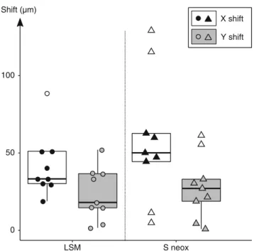
The mean shift is larger in X than Y direction for both micro-scopes (Table2, Fig.3, Online Resource5, and script no. 3 of Online Resource6): around 42 and 58μm (X), and around 24 and 28μm (Y), for the LSM and S neox respectively. The same trend can be observed on the medians. The positional repeatability varies greatly around these central tendencies: from less than 1μm (Y direction on the S neox) to more than 129μm (X direction on the S neox).
The X and Y shifts, as well as their variations, are smaller on the LSM than on the S neox.
3D surface texture
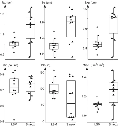
Six parameters, spanning the different categories of field pa-rameters (Online Resource4), are plotted on Fig.4; plots for
the other 23 parameters can be found in the HTML output for the statistical analysis (script no. 3 of Online Resource6). The Sa and Sq parameters are different measures of surface rough-ness (Blateyron2013). Sxp is the height difference between the average height of the surface (p = 50% material ratio) and the highest peak, excluding the 2.5% highest points (q = 97.5% material ratio). Str is a measure of isotropy; it varies between 0 (anisotropic surface) and 1 (isotropic surface). Std calculates the main direction of the surface, but is obviously only relevant for anisotropic surfaces, which is not the case here (Str > 0.6). Vmc is the volume of material (i.e., below the surface), excluding the 10% lowest (p = 10%) and 20% highest (q = 80%) points.
The variation in the measurement of surface texture be-tween the repeated measurements is substantial for most pa-rameters (Fig.4; Online Resources5–7). In other words, all quantified properties of the surface texture (height, roughness, isotropy, volume...; Online Resource4) are impacted by the
X-0 50 100 LSM S neox Shift (µm) X shift Y shift
Fig. 3 Boxplots of X/Y shifts on both microscopes. The boxes represent the interquartile range (IQR), i.e., between the 25th and 75th percentile, with the median shown as a thick horizontal line. The bars extend up to 1.5 IQR on each side of the box. Empty symbols represent outliers (points beyond 1.5 IQR). The points are spread horizontally within each group so that none are superimposed for readability
Table 2 Descriptive statistics of X/Y shifts on both microscopes
X (μm) Y (μm)
Microscope n Min Max Mean Median SD Min Max Mean Median SD
LSM 9 18.85 88.73 41.84 33.30 20.39 1.57 52.11 23.57 18.07 17.02
S neox 9 5.01 129.30 58.46 50.23 41.44 0.79 61.37 28.09 27.10 20.39 n sample size, min minimum, max maximum, SD standard deviation
Y shift from the coordinate system functionality. The variabil-ity between the measurements is larger on the S neox than on the LSM for 20 out of 29 ISO 25178 parameters, spanning all categories except height parameters and probably resulting from the larger X-Y shift.
Discussion
The proposed coordinate system functionality is articulated into two main steps. First, three ceramic beads are adhered onto the sample’s surface to serve as reference markers. In case of experimental samples, epoxy resin is preferred so that the beads are permanently and strongly adhered. It is indeed important that the beads are not removed during the ex-periments, as the coordinate system cannot be recreated if one or more beads get detached or displaced. For archeological samples, Paraloid B72 can be used because it is easily reversible. However, this is meaningful only if the beads can be adhered for at least two sequential im-aging acquisitions before being removed.
Second, the software packages of the confocal micro-scopes use these markers to define a coordinate system on the sample. Every scan is then relative to this coordinate
system and it is therefore possible to automatically relo-cate the position.
Comparison of software packages
The same experimental stone tool was scanned with two con-focal microscopes: a Zeiss LSM 800 MAT operated with the ZEN blue software package (together with the Shuttle-and-Find module), and a Sensofar S neox with SensoSCAN soft-ware. Both software packages offer a coordinate system func-tionality but the workflow is different and most variations result from a different original application. This part of the Sensofar software was developed to be used as a template, i.e., to prepare a routine to analyze different samples in iden-tical ways. The Shuttle-and-Find module of Zeiss was devel-oped for correlative microscopy, i.e., for imaging the same spot on a given sample with different pieces of equipment (e.g., light and scanning electron microscopes [SEM]). This is why SensoSCAN needs a template for the acquisition pa-rameters (Bsingle measurement recipe^, SMR), while the ac-quisition settings can be adjusted for each measurement and the coordinate system is calibrated before acquisition in ZEN blue. The SensoSCAN workflow could become problematic if the sample or its orientation has changed significantly, so that the z-range is too small for the new acquisition. In this case, 0.9 1.1 1.3 Sa (µm) 1.2 1.4 1.6 0.5 0.6 0.7 0.8 LSM S neox 0 50 100 150 2.5 3.0 3.5 1.0 1.2 1.4 Sq (µm) Sxp (µm) Str (no unit) Std (°) Vmc (µm3/µm2) LSM S neox LSM S neox
Fig. 4 Boxplots of selected ISO 25178 parameters: Sa, Sq, Sxp, Str, Std, and Vmc. See Fig.3for details on boxplots and symbols
the z-range should be increased in advance in the SMR to account for this possibility; this is why we set it to 60μm (Table1). The very fast acquisition of the S neox, as compared to the LSM, makes this solution practical. Additionally, each position can be assigned a different SMR, so that each position can be acquired with appropriate settings. On the other hand, while it is possible to plan several acquisitions on the same sample in ZEN blue (with another optional module), each acquisition must be run with the same settings.
Some other differences are noteworthy. The size of the crosshair is fixed in ZEN blue while the diameter of the circle can be adjusted to fit the diameter of beads in SensoSCAN, which should improve the positional repeatability, although the X-Y deviation was observed to be higher for the S neox (Table2). The Shuttle-and-Find module (Zeiss) also offers more possibilities: the coordinate system can be (1) mirrored so that the same system can be applied to originals, molds, and casts, and (2) transferred between different microscopes (light, digital, and confocal microscopes, and SEM) as long as each of them features a motorized XY stage and the Shuttle-and-Find module. Finally, in SensoSCAN, the stage moves auto-matically to where it expects the next reference marker. We did not find an option to deactivate this behavior that could be dangerous for some samples and the objectives, as the objec-tive could then crash into the sample. This behavior can be turned off in ZEN blue (Online Resource2, step 6a).
Accuracy of the method
The positional repeatability of the coordinate system function-ality depends on several factors: positional repeatability of the motors of the XY stage, rounding errors of the algorithms, and transformations unaccounted for (rotation and tilt, see below). The mean absolute positional repeatability (combined mean X and Y shifts via Pythagoras’ formula), taking into account all these factors, is 48.02μm for the LSM and 64.86 μm for the S neox. However, these values should be considered relative to the acquired field of view, larger with the S neox. The relative positional repeatability could be defined as the absolute re-peatability divided by the field of view diagonal, resulting in a unit-less value. This gives 13.29% on the LSM and 14.77% on the S neox. Therefore, a deviation of about 14% of the field of view can be expected when using the coordinate system functionality on both microscopes. We expect that the posi-tional repeatability of microscopes from other manufacturers will be in the same range.
Ideally, the positional repeatability should be as small (i.e., small deviation) as possible, but practical and technical con-straints limit it to 14% of the field of view. While this value might seem too large, we argue it still represents an improve-ment over visual relocation, because (1) it is faster and can be applied on every sample routinely, (2) it does not depend on the recognition of features that might be removed through
wear formation during experiments, or that might not be rec-ognizable or look differently with different pieces of equip-ment, and (3) after the approximate position is found again with the functionality, fine visual adjustments could still be performed quickly to improve the relocation.
To our knowledge, there are only three studies that applied ISO 25178 parameters (Sq) to a set of experimental flints used on different worked materials. Evans and Macdonald (2011) used their experimental tools on antler, dry hide, fresh hide, greasy hide, and wood and acquired their surface topography with a laser-scanning confocal microscope (LSCM). Their Fig. 3b shows the means ± 2 standard deviations for each worked material, calculated from 3.8 and 10.1μm areas ex-tracted from the acquired surfaces. The doubled standard de-viation of Sq from the LSM (Online Resource7) would not blur the differences on the large areas between the worked materials. The measured variation of Sq on the S neox is larger, so that the different worked materials would be indis-tinguishable; the difference between unused and used samples would also vanish. Macdonald (2014) used experimental flints on antler, wood, hide, meat, and wheat and imaged their surfaces with focus variation microscopy. Based on her Table 3, it seems that the variation in Sq from the LSM would likely still allow the distinction between the worked materials, while the variability from the S neox would probably blur the differences. Unfortunately, Ibáñez et al. (2018) published only the results of their discriminant analy-sis; therefore, Sq values cannot be compared.
However, the Sq values from these other studies (Evans and Macdonald2011; Macdonald2014) are not directly com-parable to ours because the size of the analyzed areas and the processing steps are different. Moreover, these studies focused on polished areas, where Sq is expected to be lower, while we analyzed the whole image frame. So it remains to be tested whether the variations in ISO parameters due to the coordinate system repeatability would indeed mask potential differences between worked materials, use duration, applied forces, or any other experimental variable.
Limitations and future improvements
The application of reference markers on the sample as present-ed here with adhesives and ceramic beads is already easy and cheap, but it can be further improved. The ratio of epoxy resin and hardener is difficult to measure for the small quantities needed to adhere a few beads on a few samples. So there is usually a lot of waste to ensure adequate quantities for effi-cient mixing. An alternative would be to work with UHU Endfest epoxy resin in dual-barrel cartridges with mixing tips. While the process worked well with epoxy resin, the Paraloid B72 proved difficult to work with because of its short curing time and, in high dilution, low viscosity, leading to larger-than-needed areas covered in glue (Fig.1b). Adjusting
the ratio of Paraloid B72 to ethyl acetate will surely improve the applicability of this glue, and therefore the applicability of this process to archeological samples.
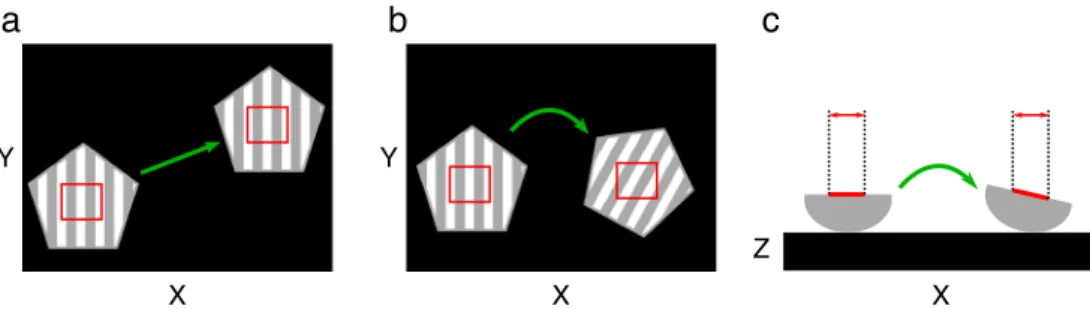
The orientation of a sample on a microscope XY stage can vary along three geometric transformations: translation (linear movement in the horizontal XY plane), rotation (circular movement in the horizontal XY plane), and tilt (inclination relative to the horizontal XY plane). The software packages used here can mathematically correct for translation of the sample on the stage: it does not matter where the sample is located on the stage (Fig.5a). However, rotation on the stage is only partially accounted for: the center of the field of view is located on the same point of the sample, but the field of view is rotated, meaning that different parts of the sample are im-aged (Fig.5b). Finally, tilt cannot be fully corrected because the size of the imaged part of the sample varies with tilt (Fig.
5c). Furthermore, the software packages used here do not correct for tilt but account only for horizontal transformations (translation and rotation). The positional repeatability of the coordinate system therefore depends greatly on the precision of the re-positioning (rotation and tilt) on the stage. A molded support can be used to reproducibly orientate (tilt) the sample on the microscope stage (similar to Fig.2). Alternatively, or additionally, a two-axis goniometer and/or a rotational stage with micrometer screws would allow the precise reorientation of the sample.
As a final note, defining the area of interest before running the experiment as shown here is not without its problems. Most use-wear studies analyze areas showing polish (i.e., shiny, flattened surfaces in light microscopy; e.g., Marreiros et al.2015 and references therein) because the polished areas are assumed to represent the most distinctive wear. However, the extent of these polished areas depends on many factors (among others, duration of use, force applied, and worked material; Marreiros et al.2015
and references therein). This implies that it is not possible to know before the experiment where polish is going to develop on the sample. Three strategies can be employed to deal with this problem, in order to be able to compare the surface topography before, during, and after an experiment. First, a sufficient number of areas can be analyzed before the experiment so that at least one will show use-wear at the end of the experiment; this is
likely not an efficient approach. Second, algorithms could be used to automatically extract and analyze the polished areas only within a large enough acquired surface, as Evans et al. (2014) did, with partial success. Finally, visual identification of polish probably represents the end stage of a continuous wear process (e.g., Grace 1989); earlier wear stages, where polish cannot be observed with light microscopy or SEM, could still be quantitatively distinctive of different uses (e.g., worked ma-terial, force, duration).
Conclusions
In this study, we presented a simple protocol to create a coor-dinate system on a sample that can be used to automatically relocate a given position on such sample. The workflow can be split into three main steps: (1) adhere three ceramic beads onto the sample that will serve as reference markers, (2) set up the coordinate system and define the position(s) of interest on the sample, and (3) use the coordinate system functionality to automatically relocate these position(s).
We first demonstrated the applicability of this approach on an experimental flint blade by adhering beads with epoxy resin onto the sample. We also showed that the beads can be attached to archeological samples if Paraloid B72 is used, because this polymer is reversible with solvents such as ace-tone or ethyl acetate. We then applied and tested this method with two confocal microscopes: a laser-scanning confocal mi-croscope manufactured by Carl Zeiss Microscopy GmbH (LSM 800 MAT) and an optical profilometer by Sensofar Metrology (S neox). This method can be used with any mi-croscope with a motorized XY stage and the same software functionalities: all types of microscopes from Zeiss; all profilometers from Sensofar (S neox and its predecessors) and Leica (DCM8); the Olympus LEXT presumably has a similar functionality, too. Positional repeatability is likely to vary depending on the equipment due to the motors’ repeat-ability and software algorithms.
As all methods, this method has limitations and the relative positional repeatability of about 14% of the field of view might seem large. On the other hand, it still represents a great
X Y
a
X Yb
X Zc
Fig. 5 Schematic drawing of translation (a), rotation (b), and tilt (c). A component of translation is included in b and c as well, for readability. Black = microscope stage, red = field of view, green arrows =
transformation, gray stripped pentagon = sample, X-Y-Z = microscope directions (X and Y axes define the horizontal plane, and Z is the vertical axis)
improvement over visual relocation, especially for quantita-tive use-wear analyses. In some cases, it can be used as a first step. Fine adjustments could be made visually so that the position(s) can be relocated more quickly. Alternatively, the B4D Series Analysis^ module of ConfoMap/MountainsMap could be used to automatically perform the fine alignments. However, if the surface has changed too much (e.g., due to experimentation) or if the different pieces of equipment image the sample in ways that are difficult to compare visually (e.g., light microscope vs. SEM), this coordinate system function-ality is the best option.
We regard this coordinate system functionality as an im-portant step toward repeatability and reproducibility in exper-imental studies. With this method, it is not only possible and easier to analyze the same location(s) on a sample during sequential experiments, but also to re-analyze the same sample in a comparable way, either with different pieces of equipment for further analysis or by different researchers. We therefore hope that this protocol will contribute to the development of reproducible experimental programs and archeological re-search, especially in, but not limited to, use-wear analysis. Acknowledgments We thank Sigmund Lindner GmbH for providing us the ceramic beads used for the coordinate system, and BTC Europe GmbH for the detergent used to clean the samples. We also thank Adam M. Platteis (Sensofar Metrology) and Dr. Matthias Vaupel (Carl Zeiss Microscopy GmbH) for their help with the microscopes. Funding This research has been supported within the Römisch-Germanisches Zentralmuseum– Leibniz Research Institute for Archeology by German Federal and Rhineland Palatinate funding (SondertatbestandBSpurenlabor^) and is publication no. 1 of the TraCEr laboratory. AR and RI thank New York University for funding the Anthrotopography Laboratory.
Compliance with ethical standards
Conflict of interest The authors declare that they have no conflict of interest.
Open Access This article is distributed under the terms of the Creative C o m m o n s A t t r i b u t i o n 4 . 0 I n t e r n a t i o n a l L i c e n s e ( h t t p : / / creativecommons.org/licenses/by/4.0/), which permits unrestricted use, distribution, and reproduction in any medium, provided you give appropriate credit to the original author(s) and the source, provide a link to the Creative Commons license, and indicate if changes were made. Publisher’s note Springer Nature remains neutral with regard to jurisdic-tional claims in published maps and institujurisdic-tional affiliations.
References
Allaire JJ, Xie Y, McPherson J et al (2018) rmarkdown: Dynamic Documents for R. R package version 1.11. https://CRAN.R-project.org/package=rmarkdown. Accessed 27 Sep 2018
Asryan L, Ollé A, Moloney N (2014) Reality and confusion in the rec-ognition of post-depositional alterations and use-wear: an experi-mental approach on basalt tools. J Lithic Stud 1:9–32.https://doi. org/10.2218/jls.v1i1.815
Bengtsson H (2018) R.utils: Various Programming Utilities. R package version 2.7.0.https://CRAN.R-project.org/package=R.utils. Accessed 27 Sep 2018
Benito-Calvo A, Arroyo A, Sánchez-Romero L, Pante M, de la Torre I (2018) Quantifying 3D micro-surface changes on experimental stones used to break bones and their implications for the analysis of early stone age pounding tools. Archaeometry 60:419–436.
https://doi.org/10.1111/arcm.12325
Blateyron F (2013) The areal feature parameters. In: Leach R (ed) Characterisation of areal surface texture. Springer Berlin Heidelberg, Berlin, Heidelberg, pp 45–65
Bofill M, Procopiou H, Vargiolu R, Zahouani H (2013) Use-wear analysis of Near Eastern prehistoric Grinding stones. In: Anderson PC, Cheval C, Durand A (eds) Regards croisés sur les outils liés au travail des végétaux. An interdisciplinary focus on plant-working tools. APDCA, Antibes, pp 219–236
Chabot J, Dionne M-M, Paquin S (2017) High magnification use-wear analysis of lithic artefacts from Northeastern America: creation of an experimental database and integration of expedient tools. Quat Int 427:25–34.https://doi.org/10.1016/j.quaint.2015.11.061
Evans AA, Donahue RE (2005) The elemental chemistry of lithic microwear: an experiment. J Archaeol Sci 32:1733–1740.https:// doi.org/10.1016/j.jas.2005.06.010
Evans AA, Donahue RE (2008) Laser scanning confocal microscopy: a potential technique for the study of lithic microwear. J Archaeol Sci 35:2223–2230.https://doi.org/10.1016/j.jas.2008.02.006
Evans AA, Macdonald D (2011) Using metrology in early prehistoric stone tool research: further work and a brief instrument comparison. Scanning 33:294–303.https://doi.org/10.1002/sca.20272
Evans AA, Macdonald DA, Giusca CL, Leach RK (2014) New method development in prehistoric stone tool research: evaluating use dura-tion and data analysis protocols. Micron 65:69–75.https://doi.org/ 10.1016/j.micron.2014.04.006
Galimova M, Sitdikov A (2017) Prehistoric flint scrapers or gun-lock flints? Experimental and use-wear criteria (according to archaeology of Kazan, Tatarstan). Quat Int 427:74–79.https://doi.org/10.1016/j. quaint.2015.12.006
Grace R (1989) Interpreting the function of stone tools: the quantification and computerisation of microwear analysis. B.A.R. Internation Series 474. Archaeopress, Oxford
Højsgaard S, Halekoh U (2018) doBy: Groupwise Statistics, LSmeans, Linear Contrasts, Utilities. R package version 4.6–2.https://CRAN. R-project.org/package=doBy. Accessed 27 Sep 2018
Ibáñez JJ, Lazuen T, González-Urquijo J (2018) Identifying experimental tool use through confocal microscopy. J Archaeol Method Theory.
https://doi.org/10.1007/s10816-018-9408-9
International Organization for Standardization (1996) ISO 4288 – Geometrical product specifications (GPS)– Surface texture: Profile method– Rules and procedures for the assessment of surface texture
International Organization for Standardization (1997) ISO 4287 – Geometrical product specifications (GPS)– Surface texture: Profile method– Terms, definitions and surface texture parameters International Organization for Standardization (2012) ISO 25178-2– geometrical product specifications (GPS)– surface texture: areal – part 2: terms, Definitions and surface texture parameters
Key AJM, Stemp WJ, Morozov M, Proffitt T, de la Torre I (2015) Is loading a significantly influential factor in the development of lithic microwear? An experimental test using LSCM on basalt from Olduvai Gorge. J Archaeol Method Theory 22:1193–1214.https:// doi.org/10.1007/s10816-014-9224-9
Leach R (ed) (2013) Characterisation of areal surface texture. Springer-Verlag, Berlin Heidelberg
Macdonald DA (2014) The application of focus variation microscopy for lithic use-wear quantification. J Archaeol Sci 48:26–33.https://doi. org/10.1016/j.jas.2013.10.003
Marreiros JM, Mazzucco N, Gibaja JF, Bicho N (2015) Macro and micro evidences from the past: the state of the art of archeological use-wear studies. In: Marreiros JM, Gibaja Bao JF, Ferreira Bicho N (eds) Use-wear and residue analysis in archaeology. Springer International Publishing, Cham, pp 5–26
Martisius NL, Sidéra I, Grote MN, Steele TE, McPherron SP, Schulz-Kornas E (2018) Time wears on: assessing how bone wears using 3D surface texture analysis. PLoS One 13:e0206078.https://doi.org/ 10.1371/journal.pone.0206078
Ollé A, Vergès JM (2014) The use of sequential experiments and SEM in documenting stone tool microwear. J Archaeol Sci 48:60–72.https:// doi.org/10.1016/j.jas.2013.10.028
Pedergnana A, Asryan L, Fernández-Marchena JL, Ollé A (2016) Modern contaminants affecting microscopic residue analysis on stone tools: a word of caution. Micron 86:1–21.https://doi.org/10. 1016/j.micron.2016.04.003
Portillo M, Bofill M, Molist M, Albert RM (2013) Phytolith and use-wear functional evidence for grinding stones from the Near East. In: Anderson PC, Cheval C, Durand A (eds) Regards croisés sur les outils liés au travail des végétaux. An interdisciplinary focus on plant-working tools. APDCA, Antibes, pp 205–218
Queffelec A, Rosso D, d’Errico F (2018) The use of ochre 40,000 years ago in Africa. Sensofar Metrology, Barcelona
R Core Team (2018) R: a language and environment for statistical com-puting. R Foundation for Statistical Computing, Vienna, Austria. Version 3.5.2.https://www.R-project.org/. Accessed 27 Sep 2018 Sano K, Oba M (2015) Backed point experiments for identifying
mechanically-delivered armatures. J Archaeol Sci 63:13–23.
https://doi.org/10.1016/j.jas.2015.08.005
Stemp WJ, Stemp M (2001) UBM laser profilometry and lithic use-wear analysis: a variable length scale investigation of surface topography. J Archaeol Sci 28:81–88.https://doi.org/10.1006/jasc.2000.0547
Stemp WJ, Stemp M (2003) Documenting stages of polish development on experimental stone tools: surface characterization by fractal
geometry using UBM laser profilometry. J Archaeol Sci 30:287– 296.https://doi.org/10.1006/jasc.2002.0837
Stemp WJ, Lerner HJ, Kristant EH (2013) Quantifying microwear on experimental Mistassini quartzite scrapers: preliminary results of exploratory research using LSCM and scale-sensitive fractal analy-sis. Scanning 35:28–39.https://doi.org/10.1002/sca.21032
Stemp WJ, Morozov M, Key AJM (2015) Quantifying lithic microwear with load variation on experimental basalt flakes using LSCM and area-scale fractal complexity (Asfc). Surf Topogr Metrol Prop 3: 034006.https://doi.org/10.1088/2051-672X/3/3/034006
Stemp WJ, Lerner HJ, Kristant EH (2018) Testing area-scale fractal com-plexity (Asfc) and laser scanning confocal microscopy (LSCM) to document and discriminate microwear on experimental quartzite scrapers. Archaeometry 60:660–677.https://doi.org/10.1111/arcm. 12335
Walker A (2018) openxlsx: Read, Write and Edit XLSX Files. R package version 4.1.0.https://CRAN.R-project.org/package=openxlsx. Accessed 27 Sep 2018
Watson AS, Gleason MA (2016) A comparative assessment of texture analysis techniques applied to bone tool use-wear. Surf Topogr Metrol Prop 4:024002.https://doi.org/10.1088/2051-672X/4/2/ 024002
Werner JJ (2018) An experimental investigation of the effects of post-depositional damage on current quantitative use-wear methods. J Archaeol Sci Rep 17:597–604.https://doi.org/10.1016/j.jasrep. 2017.12.008
Wickham H (2016) ggplot2: Elegant Graphics for Data Analysis. Springer, New York
Xie Y (2014) knitr: A Comprehensive Tool for Reproducible Research in R. In: Stodden V, Leisch F, Peng RD (eds) Implementing Reproducible Computational Research. Chapman and Hall/CRC, Boca Raton
Xie Y (2015) Dynamic Documents with R and knitr, 2nd edn. Chapman and Hall/CRC, Boca Raton
Xie Y (2018) knitr: A General-Purpose Package for Dynamic Report Generation in R. R package version 1.21.https://yihui.name/knitr/. Accessed 27 Sep 2018