O USO INDEVIDO DA ALTERAÇÃO DA SINTAXE NAS ANÁLISES POST-HOC DE GEE E ANOVA NO SPSS

(1)

THE MISUSE OF SYNTAX ALTERATION FOR GEE AND ANOVA POST-HOC

ANALYSES IN SPSS

João Pedro Nunes¹*, Giovanna Fachetti Frigoli²

¹. Physical Education and Sport Center, Londrina State University, Brazil; - [email protected] ². Biological Sciences Center, Londrina State University, Brazil.

Abstract

The online support of IBM SPSS proposes that users

alter the syntax when performing post-hoc analyses

for interaction effects of ANOVA tests. Other

authors also suggest altering the syntax when

performing GEE analyses. This being done, the

number of possible comparisons (k value) is also

altered, therefore influencing the results from

statistical tests that k is a component of the formula,

such as repeated measures-ANOVA and Bonferroni

post-hoc of ANOVA and GEE. This alteration also

exacerbates type I error, producing erroneous

results and conferring potential misinterpretations

of data. Reasoning from this, the purpose of this paper is to report the misuse and improper

handling of syntax for ANOVAs and GEE post-hoc analyses in SPSS and to illustrate its

consequences on statistical results and data interpretation.

Resumo

O suporte on-line do IBM SPSS propõe que os usuários alterem a sintaxe ao executar análises

post-hoc para efeitos de interação de testes ANOVA. Outros autores também sugerem alterar a

sintaxe ao realizar análises GEE. Assim sendo, o número de possíveis comparações (valor de k)

também é alterado, influenciando, portanto, os resultados dos testes estatísticos de que k é um

componente da fórmula, como na ANOVA de medidas repetidas e nos post-hoc de ANOVA e

GEE. Essa alteração também agrava o erro do tipo I, produzindo resultados errôneos e

conferindo possíveis interpretações errôneas dos dados. Com base nisso, o objetivo deste artigo

é relatar o uso indevido e o manuseio inadequado da sintaxe nas análises post-hoc de ANOVAs

e GEE no SPSS e ilustrar suas consequências nos resultados estatísticos e na interpretação dos

dados

.

INTRODUÇÃO

Statistical tools help to store, organize, and analyze data. Statistical package programs such as SPSS, Statistica, JASP, SigmaPlot, MedCalc, R, etc., facilitate the performance of such tasks, whose purpose is to do

this most accurate as possible. Its use is important to the field of quantitative and experimental sciences; particularly in health sciences, statistical analyses are used to compare the efficacy of a drug to a control situation, for example. For this comparison, there must be at least Info Recebido: 12/2019 Publicado: 04/2020 DOI: 10.29247/2358-260X.2020v7i1.4164 ISSN: 2358-260X Palavras-Chave

estatística; bioestatística; análise de comparação múltipla; precisão Keywords:

statistic; biostatistics; multiple comparison analysis; accuracy

(2)

two measurements in two different timeframes (pre and post-treatment) for both groups (drug vs. control). Thus, there are two fixed factors to be compared: time and group. The most common statistical tests for such time*group comparisons are general and generalized linear model equations (e.g. analysis of variance; ANOVA), when statistical assumptions are met.

In SPSS, the execution of these equations takes place in a simple way, so that it is only necessary to insert the desired variables in recommended boxes. The output provides statistical results (statistical F, and P values) of the main effect of time, main effect of group, and the effect of the interaction time*group; in other words, it presents results of comparisons between different times of data collection (pre- vs. post-intervention), between groups (group 1 vs. group 2), and verify whether they

have equal or different results for desired variable over the time. However, for ANOVA tests, the SPSS presents only comparisons of main effects and does not allow the execution of multiple comparisons (post-hoc) for the interaction effect. The mean and 95% confidence intervals (CIs) of estimated marginal means (EMM) for time*group results are created, allowing only visual inspection of these values so that neither the comparisons between them are performed, nor P values are presented. In this sense, the guide formulated by IBM SPSS support, available online (IBM, 2016a, b), recommends changing the program’s syntax to solve this problem, providing some comparisons. The recommendation acts according to the following example (IBM, 2016a, b):

Original syntax:

/EMMEANS = TABLES(time) COMPARE ADJ(BONFERRONI) /EMMEANS = TABLES(group) COMPARE ADJ(BONFERRONI)

/EMMEANS = TABLES(time*group) Altered syntax:

/EMMEANS = TABLES(time*group) COMPARE(time) ADJ(BONFERRONI) /EMMEANS = TABLES(time*group) COMPARE(group) ADJ(BONFERRONI) In addition, Guimarães and Hirakata

(GUIMARÃES; HIRAKATA, 2013) recommended altering the command-line syntax for generalized linear models (specifically generalized estimated equations; GEE), as similar as did by IBM SPSS support (IBM, 2016a, b). Guimarães and Hirakata suggested that, without this alteration, the originally available output provided by the program is extensive and “difficult to understand” (GUIMARÃES; HIRAKATA, 2013), and with such alteration, desired comparisons for interaction effect could be performed in a potentially clearer way.

However, when using these recommended syntax alterations (GUIMARÃES; HIRAKATA, 2013; IBM, 2016a, b), the mean values of the groups at different times are compared separately, as well as the mean values of each time between different groups. The correct way should be to compare the values altogether. With this, a reduction in the possible number of comparisons is done. Such number is reported as k, and it is a component of post-hoc formulas._{. For example,}

Bonferroni post-hoc adjusts the α (e.g. 0.05) for accepting significance diving α by k. The k value is

(3)

calculated by multiplying the number of means to be compared; then this result should be squared, and then subtracted by one unit from this result, and divided by 2. E.g., In 2x3 comparisons, k value is 15: 2x3 = 6... (6^2 - 6)/2 = 15.

By changing k value, it influences the analyses, may confer erroneous results and misinterpretation of data. In this sense, the purpose of this paper is to alert the misuse and improper handling of the syntax for ANOVA and GEE post-hoc analyses in SPSS and to show its consequences onto statistical results [P values, standard error (SE) and confidence intervals of the differences between comparisons] and data interpretation.

Methods

A data set was designed to illustrate why improper alteration of the syntax in SPSS for making multiple comparisons leads to incorrect results depending on post-hoc to be used: 2 groups with 20 subjects each performing two distinct protocols of resistance training (G1 and G2) were evaluated in a strength test at baseline (T1), and after 5 (T2) and 10 weeks (T3) of intervention. The spreadsheet of the data is available in Supplementary Material.

A repeated measures-ANOVA (rmANOVA) with two fixed factors, group (G1, G2) and time (T1, T2, T3), was performed to verify differences within and between groups. Firstly, in SPSS, a rmANOVA was performed with LSD post-hoc with proposed alterations in syntax (IBM, 2016b), which does not adjust the α for significance acceptance. Subsequently, a Bonferroni post-hoc was performed with alterations in the syntax. The same steps were performed for 2wANOVA (IBM, 2016a).

Since SPSS does not depict all possible comparisons on the output but only between groups at different times and between times for each group, in order to obtain all comparisons, Bonferroni post-hocs were performed in three other statistical softwares: Statistica, JASP, and Jamovi. Additionally, a “simulated” Bonferroni post-hoc after a 2wANOVA was performed in SPSS with following procedures: in the adjustment label for multiple comparisons, LSD was selected (equivalent to no adjustment), however, the α to accept significance was altered from 0.05 (default) to 0.003333, as a result of the α divided by k value (which is 15, in this case). This would offer the possibility to certify whether comparisons (only those available in SPSS) present equal results between the softwares; which indeed did.

For GEE analysis in SPSS, the type of model was defined as linear, after that, there were performed post-hocs of LSD and Bonferroni with and without syntax alterations (GUIMARÃES; HIRAKATA, 2013). Significance was set at P <0.05. The data was stored in Excel (v. 15.0, Excel for Microsoft Office 2013, Redmond, WA, USA), and analyzed in IBM SPSS Statistics (v. 23.0, IBM Corp., Armonk, NY, USA), STATISTICA software (v. 10.0, Statsoft Inc., Tulsa, OK, USA), JASP (Jasp Stats, Amsterdam, Netherlands), Jamovi (v. 0.9, The Jamovi Project).

Results

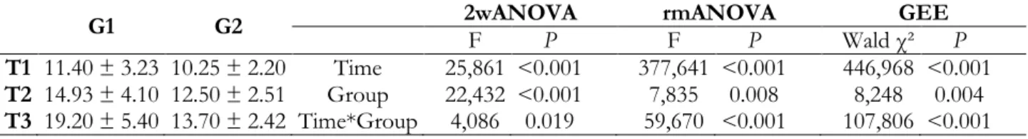
Values for both G1 and G2 in T1, T2, and T3 are presented in Table 1. Significant main effects of time and group and time*group effect were observed with 2wANOVA, rmANOVA, and GEE. The F and P values for ANOVAs, and Wald χ², and P for GEE are

(4)

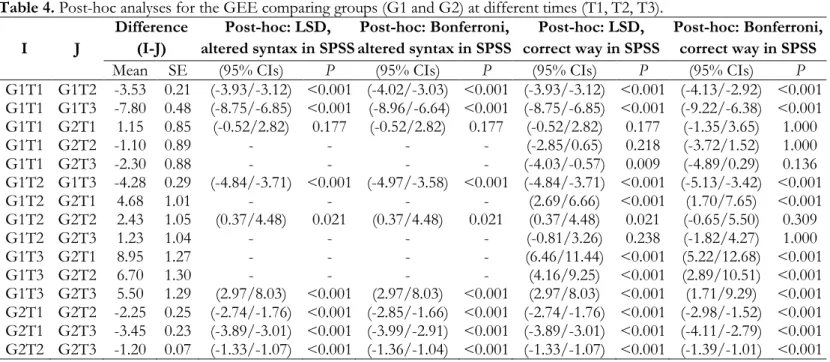
also presented in Table 1. Post-hocs for 2wANOVA, rmANOVA, and GEE analyses are presented in Table 2, Table 3, and Table 4, respectively.

Table 1. ANOVAs and GEE main effects and interaction for values of the illustrative data.

G1 G2 2wANOVA _F _P rmANOVA _F _P _{Wald χ²}GEE _P

T1 11.40 ± 3.23 10.25 ± 2.20 Time 25,861 <0.001 377,641 <0.001 446,968 <0.001

T2 14.93 ± 4.10 12.50 ± 2.51 Group 22,432 <0.001 7,835 0.008 8,248 0.004

T3 19.20 ± 5.40 13.70 ± 2.42 Time*Group 4,086 0.019 59,670 <0.001 107,806 <0.001

Blank spaces in tables are due to that SPSS does not offer such comparisons. Notably, 95% CIs and P were influenced by proposed alteration for all three tests, 2wANOVA (Table 2), rmANOVA (Table 3), and GEE (Table 4). In 2wANOVA and GEE, the altered syntax induces erroneous results only with Bonferroni

post-hoc, while with post-hoc least significant difference (LSD) not. In the rmANOVA test, when the post-hoc is performed with the syntax change (either LSD or Bonferroni) the values of 95% CIs and P are affected, as well as the SE of the difference between the values compared.

Table 2. Post-hoc analyses for the 2wANOVA comparing groups (G1 and G2) at different times (T1, T2, T3).

I J Difference (I-J) altered syntax in SPSS Post-hoc: LSD, Post-hoc: Bonferroni, altered syntax in SPSS Post-hoc: LSD, correct way Post-hoc: Bonferroni, correct way

Mean SE (95% CIs) P (95% CIs) P (95% CIs) P (95% CIs) P

G1T1 G1T2 -3.53 1.11 (-5.72/-1.33) 0.002 (-6.21/-0.84) 0.006 (-5.72/-1.33) 0.002 (-6.84/-0.21) 0.028 G1T1 G1T3 -7.80 1.11 (-9.99/-5.61) <0.001 (-10.49/-5.11) <0.001 (-9.99/-5.61) <0.001 (-11.12/-4.48) <0.001 G1T1 G2T1 1.15 1.11 (-1.04/3.34) 0.301 (-1.04/3.34) 0.301 (-1.04/3.34) 0.301 (-2.17/4.47) 1.000 G1T1 G2T2 -1.10 1.11 - - - - (-3.29/1.09) 0.322 (-4.42/2.22) 1.000 G1T1 G2T3 -2.30 1.11 - - - - (-4.49/-0.11) 0.040 (-5.62/1.02) 0.598 G1T2 G1T3 -4.28 1.11 (-6.47/-2.08) <0.001 (-6.96/-1.59) 0.001 (-6.47/-2.08) <0.001 (-7.59/-0.96) 0.003 G1T2 G2T1 4.68 1.11 - - - - (2.48/6.87) <0.001 (1.36/7.99) 0.001 G1T2 G2T2 2.43 1.11 (0.23/4.62) 0.030 (0.23/4.62) 0.030 (0.23/4.62) 0.030 (-0.89/5.74) 0.456 G1T2 G2T3 1.23 1.11 - - - - (-0.97/3.42) 0.270 (-2.09/4.54) 1.000 G1T3 G2T1 8.95 1.11 - - - - (6.76/11.14) <0.001 (5.63/12.27) <0.001 G1T3 G2T2 6.70 1.11 - - - - (4.51/8.89) <0.001 (3.38/10.02) <0.001 G1T3 G2T3 5.50 1.11 (3.31/7.69) <0.001 (3.31/7.69) <0.001 (3.31/7.69) <0.001 (2.18/8.82) <0.001 G2T1 G2T2 -2.25 1.11 (-4.44/-0.06) 0.044 (-4.94/0.44) 0.133 (-4.44/-0.06) 0.044 (-5.57/1.07) 0.664 G2T1 G2T3 -3.45 1.11 (-5.64/-1.26) 0.002 (-6.14/-0.76) 0.007 (-5.64/-1.26) 0.002 (-6.77/-0.13) 0.035 G2T2 G2T3 -1.20 1.11 (-3.39/0.99) 0.280 (-3.89/1.49) 0.841 (-3.39/0.99) 0.280 (-4.52/2.12) 1.000

(5)

Table 3. Post-hoc analyses for the rmANOVA comparing groups (G1 and G2) at different times (T1, T2, T3). I J Difference (I-J) Post-hoc: LSD, altered syntax in SPSS Post-hoc: Bonferroni, altered syntax in SPSS Post-hoc: LSD, correct way Post-hoc: Bonferroni, correct way

Mean SE (95% CIs) P SE (95% CIs) P SE (95% CI)s P SE (95% CIs) P

G1T1 G1T2 -3.53 0.24 (-4.00/-3.05) <0.001 0.24 (-4.11/-2.94) <0.001 0.29 (-4.10/-2.95) <0.001 0.29 (-4.40/-2.65) <0.001 G1T1 G1T3 -7.80 0.39 (-8.58/-7.02) <0.001 0.39 (-8.77/-6.83) <0.001 0.29 (-8.38/-7.22) <0.001 0.29 (-8.68/-6.92) <0.001 G1T1 G2T1 1.15 0.87 (-0.62/2.92) 0.196 0.87 (-0.62/2.92) 0.196 1.11 (-1.09/3.39) 0.305 1.11 (-2.31/4.61) 1.000 G1T1 G2T2 -1.10 - - - - 1.11 (-3.34/1.14) 0.326 1.11 (-4.56/2.36) 1.000 G1T1 G2T3 -2.30 - - - - 1.11 (-4.54/-0.06) 0.044 1.11 (-5.76/1.16) 0.657 G1T2 G1T3 -4.28 0.22 (-4.71/-3.84) <0.001 0.22 (-4.82/-3.73) <0.001 0.29 (-4.85/-3.70) <0.001 0.29 (-5.15/-3.40) <0.001 G1T2 G2T1 4.68 - - - - 1.11 (2.44/6.91) <0.001 1.11 (1.22/8.13) 0.002 G1T2 G2T2 2.43 1.07 (0.25/4.60) 0.030 1.07 (0.25/4.60) 0.030 1.11 (0.19/4.66) 0.034 1.11 (-1.03/5.88) 0.510 G1T2 G2T3 1.23 - - - - 1.11 (-1.01/3.46) 0.274 1.11 (-2.23/4.68) 1.000 G1T3 G2T1 8.95 - - - - 1.11 (6.71/11.19) <0.001 1.11 (5.49/12.41) <0.001 G1T3 G2T2 6.70 - - - - 1.11 (4.46/8.94) <0.001 1.11 (3.24/10.16) <0.001 G1T3 G2T3 5.50 1.32 (2.82/8.18) <0.001 1.32 (2.82/8.18) <0.001 1.11 (3.26/7.74) <0.001 1.11 (2.04/8.96) <0.001 G2T1 G2T2 -2.25 0.24 (-2.73/-1.77) <0.001 0.24 (-2.84/-1.66) <0.001 0.29 (-2.83/-1.67) <0.001 0.29 (-3.13/-1.37) <0.001 G2T1 G2T3 -3.45 0.39 (-4.23/-2.67) <0.001 0.39 (-4.42/-2.48) <0.001 0.29 (-4.03/-2.87) <0.001 0.29 (-4.33/-2.57) <0.001 G2T2 G2T3 -1.20 0.22 (-1.64/-0.76) <0.001 0.22 (-1.74/-0.66) <0.001 0.29 (-1.78/-0.62) <0.001 0.29 (-2.08/-0.32) 0.001 Table 4. Post-hoc analyses for the GEE comparing groups (G1 and G2) at different times (T1, T2, T3).

I J Difference (I-J) Post-hoc: LSD, altered syntax in SPSS Post-hoc: Bonferroni, altered syntax in SPSS Post-hoc: LSD, correct way in SPSS Post-hoc: Bonferroni, correct way in SPSS

Mean SE (95% CIs) P (95% CIs) P (95% CIs) P (95% CIs) P

G1T1 G1T2 -3.53 0.21 (-3.93/-3.12) <0.001 (-4.02/-3.03) <0.001 (-3.93/-3.12) <0.001 (-4.13/-2.92) <0.001 G1T1 G1T3 -7.80 0.48 (-8.75/-6.85) <0.001 (-8.96/-6.64) <0.001 (-8.75/-6.85) <0.001 (-9.22/-6.38) <0.001 G1T1 G2T1 1.15 0.85 (-0.52/2.82) 0.177 (-0.52/2.82) 0.177 (-0.52/2.82) 0.177 (-1.35/3.65) 1.000 G1T1 G2T2 -1.10 0.89 - - - - (-2.85/0.65) 0.218 (-3.72/1.52) 1.000 G1T1 G2T3 -2.30 0.88 - - - - (-4.03/-0.57) 0.009 (-4.89/0.29) 0.136 G1T2 G1T3 -4.28 0.29 (-4.84/-3.71) <0.001 (-4.97/-3.58) <0.001 (-4.84/-3.71) <0.001 (-5.13/-3.42) <0.001 G1T2 G2T1 4.68 1.01 - - - - (2.69/6.66) <0.001 (1.70/7.65) <0.001 G1T2 G2T2 2.43 1.05 (0.37/4.48) 0.021 (0.37/4.48) 0.021 (0.37/4.48) 0.021 (-0.65/5.50) 0.309 G1T2 G2T3 1.23 1.04 - - - - (-0.81/3.26) 0.238 (-1.82/4.27) 1.000 G1T3 G2T1 8.95 1.27 - - - - (6.46/11.44) <0.001 (5.22/12.68) <0.001 G1T3 G2T2 6.70 1.30 - - - - (4.16/9.25) <0.001 (2.89/10.51) <0.001 G1T3 G2T3 5.50 1.29 (2.97/8.03) <0.001 (2.97/8.03) <0.001 (2.97/8.03) <0.001 (1.71/9.29) <0.001 G2T1 G2T2 -2.25 0.25 (-2.74/-1.76) <0.001 (-2.85/-1.66) <0.001 (-2.74/-1.76) <0.001 (-2.98/-1.52) <0.001 G2T1 G2T3 -3.45 0.23 (-3.89/-3.01) <0.001 (-3.99/-2.91) <0.001 (-3.89/-3.01) <0.001 (-4.11/-2.79) <0.001 G2T2 G2T3 -1.20 0.07 (-1.33/-1.07) <0.001 (-1.36/-1.04) <0.001 (-1.33/-1.07) <0.001 (-1.39/-1.01) <0.001

Discussion and conclusion

The aim of this study is to present that the suggested syntax alterations (GUIMARÃES; HIRAKATA, 2013; IBM, 2016a, b) influence the results of post-hoc interaction comparisons. That because this syntax alteration directly impacts the number of possible comparisons (k) for group*time analyses. For 2wANOVA and GEE, the syntax

alterations affect only post-hoc analyzes that adjust α value from k, like in Bonferroni. This does not happen for LSD post-hoc since this is an analysis that does not adjust α values (which is not recommended since it has a higher chance for obtaining a false positive; rejecting the null hypothesis when it should not), therefore, its P values and 95% CIs are not affected. Especially in rmANOVA, the syntax alteration affects all post-hoc

(6)

analyses, since the k value is a component in the formula of this test. In these cases, altering the syntax is not recommended.

It is noteworthy that the most appropriate ANOVA to compare the database designed to illustrate this hypothetical situation is the rmANOVA since the time factor is a within-subjects factor. However, it was used in the same illustrative database for 2wANOVA and GEE to facilitate the understanding and interpretation of the results. Further illustrative database examples in which the use of the other analyses, 2wANOVA and GEE, would be more appropriate could have been used.

It can be noted that the syntax alteration in question is problematic in relation to group comparisons at different times (i.e., G1T1 vs. G2T1, G1T2 vs. G2G2, and G1T3 vs. G2T3). In the current situation, when comparing two groups using Bonferroni post-hoc with the altered syntax, the k value is altered, and its new value is 1 (G1 vs. G2) in each comparison between groups at different times, rather than 15, as it should be. Since the k value is now 1, α value is therefore not adjusted, and so the P values and the interpretation of the results will be the same as they would be if the LSD post-hoc were to be used. Moreover, it can be noted that the comparison of G1T2 vs. G2T2 is the most problematic. With Bonferroni performed with the altered syntax, the groups G1 and G2 are significantly different at T2, whereas, using the correct analysis, the groups are statistically similar. This could lead to erroneous interpretation, therefore admitting both training methods induced strength gains in a different way and that the method performed by

G1 would be better. In an analog situation, this could lead to the conclusion that the hypothetical drug “X” would be better than the hypothetical drug “Y” after 5 weeks of treatment. The negative implications of this error for the practical field are vast.

As alternatives, some strategies may be adopted. Using another statistical software (e.g., Statistica, JASP, Jamovi), which presents all, correct comparisons of post-hoc analyzes, or changing α values before performing each post-hoc comparison within the SPSS program.

References

GUIMARÃES, L. S. P.; HIRAKATA, V. N. Use of the Generalized Estimating Equation model in longitudinal data analysis. Clinical &

Biomedical Research, v. 32, n. 4, p. 503–511, 2013. .

IBM. Repeated measures ANOVA: Interpreting a significant interaction in SPSS GLM. 2016a. IBM Support (online). Disponível em:

https://www-01.ibm.com/support/docview.wss?uid=swg214 76140. Acesso em: 13 jan. 2019.

IBM. Significant interaction in ANOVA: how to obtain a simple effects test. 2016b. IBM Support (online). Disponível em:

https://www-01.ibm.com/support/docview.wss?uid=swg214 75404. Acesso em: 13 jan. 2019.