SIMPLICITY, REPRODUCIBILITY AND SCALABILITY FOR HUGE WIRELESS SENSOR NETWORK SIMULATIONS

(1)

MATHEUS LEÔNIDAS SILVA Advisor: Joubert de Castro Lima

SIMPLICITY, REPRODUCIBILITY AND SCALABILITY

FOR HUGE WIRELESS SENSOR NETWORK

SIMULATIONS

(2)

Federal University of Ouro Preto Institute of Exact Sciences Master’s degree in Computer Science

SIMPLICITY, REPRODUCIBILITY AND SCALABILITY

FOR HUGE WIRELESS SENSOR NETWORK

SIMULATIONS

Master’s thesis presented to the Post-Graduation Program in Computer Science of the Federal University of Ouro Preto, as a partial requirement to obtain a Master’s degree in Computer Science.

MATHEUS LEÔNIDAS SILVA

(3)

Catalogação: www.sisbin.ufop.br

S381s Silva, Matheus Leônidas.

Simplicity, reproducibility and scalability for huge wireless sensor network simulations [manuscrito] / Matheus Leônidas Silva. - 2018.

61f.: il.: color; grafs; tabs.

Orientador: Prof. Dr. Joubert de Castro Lima.

Dissertação (Mestrado) - Universidade Federal de Ouro Preto. Instituto de Ciências Exatas e Biológicas. Departamento de Computação. Programa de Pós-Graduação em Ciência da Computação.

Área de Concentração: Ciência da Computação.

1. Simulação (Computadores). 2. Computação de alto desempenho . 3. Sensoriamento remoto. I. Lima, Joubert de Castro. II. Universidade Federal de Ouro Preto. III. Titulo.

(4)

(5)

Resumo

Neste trabalho apresentamos duas contribuições para a literatura de redes de sensores sem fio (WSN). A primeira é um modelo geral para alcançar a reprodutibilidade no nível do kernel em simuladores paralelos. Infelizmente, os usuários devem implementar do zero como suas simulações se repetem em simuladores WSN, mas uma simulação paralela ou distribuída im-põe o princípio de concorrência, não trivial de ser implementada por não especialistas. Testes usando o simulador chamadoJSensor comprovaram que o modelo garante o nível mais restrito de reprodutibilidade, mesmo quando as simulações adotam diferentes números de threads ou diferentes máquinas em múltiplas execuções. A segunda contribuição é o simuladorJSensor, um simulador paralelo de uso geral para aplicações WSN de grande escala e algoritmos dis-tribuídos de alto nível. O JSensor introduz elementos de simulação mais realistas, como o ambiente representado por células personalizáveis e eventos de aplicação que representam fenô-menos naturais, como raios, vento, sol, chuva e muito mais. As células são colocadas em uma grade que representa o ambiente com características do espaço definido pelos usuários, como temperatura, pressão e qualidade do ar. Avaliações experimentais mostram que o JSensor tem boa escalabilidade em arquiteturas de computadores multi-core, alcançando umspeedup de 7,45 em uma máquina com 16 núcleos com tecnologiaHyper-Threading, portanto 50% dos núcleos são virtuais. O JSensor também provou ser 21% mais rápido que o OMNeT++ ao simular um modelo do tipo flooding.

(6)

Abstract

In this work we present two contributions for the wireless sensor network (WSN) literature. The first one is a general model to achieve reproducibility in kernel level of parallel simulators. Unfortunately, users must implement how their simulations repeat from scratch in WSN sim-ulators, but a parallel or distributed simulation imposes the concurrence principle, not trivial to be implemented by non-specialists. Tests using the simulator named JSensor proved that the model guarantees the most restrict level of reproducibility, even when simulations adopt different number of threads or different machines in multiple runs. The second contribution is the JSensor simulator, a parallel general purpose simulator for large scale WSN applications and high-level distributed algorithms. JSensor introduces more realistic simulation elements, such as the environment represented by customizable cells and application-events representing natural phenomena, such as lightning, wind, sun, rain and more. The cells are placed in a grid that represents the environment with characteristics of the space defined by the users, such as temperature, pressure and air quality. Experimental evaluations show that JSensor has good scalability in multi-core computer architectures, achieving a speedup of 7.45 in a machine with 16 cores with Hyper-Threading Technology, thus 50% of cores are virtual ones. JSensor also proved to be 21% faster than OMNeT++ while simulating a flooding model.

(7)

This thesis is dedicated to my father, who taught me that the best kind of knowledge to have is that which is learned for its own sake. It is also dedicated to my mother, who taught me that even the largest task can be accomplished if it is done one step at a time.

(8)

Acknowledgments

First and foremost, I have to thank my advisor, Dr. Joubert C. Lima. Without his assistance and dedicated involvement in every step throughout the process, this project would have never been accomplished. I would like to thank you very much for your support and understanding over these past years.

Getting through my thesis required more than academic support, and I have many, many people to thank for listening to and, at times, having to tolerate me over the past years. I cannot begin to express my gratitude and appreciation for their friendship.

Most importantly, none of this could have happened without my family. To my parents and my sister– it would be an understatement to say that, as a family, we have experienced some ups and downs in the past years. Every time I was ready to quit, you did not let me and I am forever grateful. This dissertation stands as a testament to your unconditional love and encouragement.

(9)

List of Figures

3.1 JSensor’s architecture . . . 16

3.2 Grid of cells. . . 18

3.3 Parallelism in JSensor . . . 23

3.4 Cell size inﬂuence. . . 23

3.5 Synchronization barriers . . . 24

3.6 Reproducibility using chunks in JSensor. . . 28

3.7 Runtime JSensor versus Sinalgo. . . 32

3.8 Runtime JSensor versus OMNeT++ . . . 33

3.9 Memory Consumption JSensor versus OMNeT++. . . 34

3.10 JSensor speedup . . . 35

3.11 Mobility performance. . . 36

3.12 Performance versus cell size. . . 36

3.13 Memory versus cell size. . . 37

3.14 Mobile phone application speedup. . . 38

3.15 Memory consumption. . . 38

3.16 Speedup air quality application. . . 39

(12)

List of Tables

2.1 Reproducibility evaluation :: Number of messages . . . 9

2.2 Reproducibility evaluation :: Mobility events . . . 9

2.3 Reproducibility evaluation :: Node deactivation . . . 10

3.1 Summary of related work features . . . 15

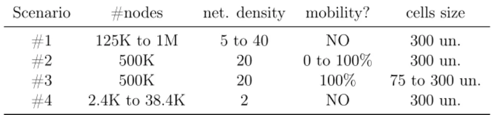
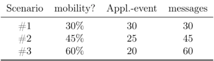
3.2 Features added for each scenario . . . 29

3.3 Features added for each scenario . . . 30

(13)

List of Algorithms

1

Runtimemain execution25

(14)

Chapter 1

Introduction

How can we analyze the water quality of a river? How can we monitor streets, cities, provinces of a country? How can we predict and prevent problems coming from earthquakes, snowstorms, ﬁre spreads and all kinds of natural disasters? How can we test some new drugs without using animals? These and many other problems are initially solved by using simulators. It is extremely expensive, and sometimes dangerous, to test initial ideas in a real environment. Thus, very often we must use simulators to achieve comfortable conﬁdence levels before real tests.

The use of simulators that until few years ago was concentrated in military and scientiﬁc domains have recently become important tools for many diverse areas, including environmental monitoring, medical (drugs utilization, clinical feedbacks, etc.), human occupations in risk, professional skills training, sports and so forth Okuda et al. (2009); Raković and Lutovac (2015); Gregory (2017). One way to simulate abstractions and their interactions is modeling them as sensor networks or precisely wireless sensor networks since some abstractions are mobile. These abstractions are named nodes and they are capable of sensing, actuating, processing, communicating and moving around the environment. Such nodes or sensors or devices, working cooperatively, are termed wireless sensor networks (WSNs) Akyildiz et al. (2002a). WSN simulators Varga and Hornig (2008a); Xue et al. (2007); Zeng et al. (1998a); Ould-Ahmed-Vall et al. (2007a) designed for huge applications Chen et al. (2005), where thousands or even millions of nodes are simulated, are becoming regular with the advance of new WSNs applications, e.g., general Internet of Things (IoT) applications Muruganandam et al. (2018), smart cities Lu et al. (2017), social sensing Ali et al. (2011) or natural environment monitoring Lin et al. (2015).

WSNs simulators for huge applications are becoming essential, as mentioned before; how-ever, standards and market-leaders simulators, such as OMNeT++, NS, GlomoSim and others Varga and Hornig (2008b); Xue et al. (2007); Zeng et al. (1998a); Ould-Ahmed-Vall et al. (2007a), do not implement environment modeling and application-events to simulate interfer-ences from external agents or natural phenomena, such as rain, sun, lightning, and so forth,

(15)

1. Introduction ₂

in Earth regions. The work Sundresh et al. (2004) detailed the importance of environment modeling in WSN simulations, despite of most simulators, in special high performance com-puting (HPC) ones, do not consider such a concept. Furthermore, some HPC simulators, like the PDNS Riley and Park (2004a), exposes its distribution complexities, such as the concept of messages of MPI Pacheco (1997) libraries, to their users, so they require high performance programming skills, a non-trivial programming knowledge for non computer scientists like the simulator users.

Another essential feature is to repeat a simulation, but this obvious requirement was not addressed by the WSN simulator literature until now. In general, the users must implement how their simulations will repeat from scratch. This development strategy implies in serious drawbacks since the users normally put together business domain issues with reproducibility issues in the simulation code. Another limitation occurred while using a parallel or distributed version of a simulator because the users will require high performance programming skills to implement their reproducibility demands. These skills include understanding concurrence principle, its benefits and limitations, a deep technical knowledge even for computer scientists. To attenuate the reproducibility problem in WSN simulators, this work presents the first generic reproducibility model to be used in kernel level of a parallel WSN simulator, this way not requiring any user interference to guarantee repeatable simulation runs, even when we change the hardware or the simulator configuration after each run (Ex. use a quadcore machine in run one and an octocore in run 2 or set the simulator with four threads in run one and with sixteen threads in run two). The model implements the concept of chunk to allow reproducibility, even when executing non-deterministic simulations in parallel. A chunk encapsulates a set of nodes and application-events, a seed to ensure a starting point to gener-ate pseudo-random numbers and a generator of pseudo-random numbers. The reproducibility model has the fundamental ideas to partition the data and the processing of a simulation among many threads, trying to achieve a fair load balancing and consequently scaling up the simulations. To evaluate its applicability and correctness, we have implemented the repro-ducibility model in Java and integrated it withJSensor simulator Silva et al. (2013); Ribeiro et al. (2012b,a). This research result is detailed in Chapter 2.

The second contribution of this work is a new WSN simulator to attenuate the limitations mentioned before. The new simulator is an extension of JSensor simulator Silva et al. (2013); Ribeiro et al. (2012b,a), thus it is a Java parallel simulator to multi-core HPC architectures that handles millions of elements, performing the evaluation of low level protocols, WSN applications and high-level distributed algorithms according to the user needs. JSensor types and operators are designed to be both simple and extensible to users, hiding HPC complexities, but also capable to scale over multi-core machines. It implements environment modeling and application-events to simulate interferences from external agents or natural phenomena.

(16)

con-1. Introduction ₃

sumption and if it is faster than a literature counterpart, precisely the OMNET++ simulator. The performance results achieved speedups of 7.45 with 16 threads running concurrently and the comparative evaluations against OMNeT++ reveled a runtime 21% faster of JSensor when simulating the ﬂooding model where the messages spreads to all connected nodes. This technological result is detailed in Chapter 3.

(17)

Chapter 2

Reproducibility in Parallel Sensor

Network Simulations

2.1 Abstract

Currently, some network simulators adopt parallel computer architectures to improve their scalability. The main problem with this strategy is guaranteeing the reproducibility transpar-ently to simulation users. To diminish this problem, in this work, we present a reproducible parallel simulation model that can be adopted in huge sensor network scenarios. This model was integrated into a parallel sensor network simulator and validated accordingly. The model is based on a chunk partition strategy, in which all simulation elements are wrapped into chunks and simulated sequentially inside each chunk. Multiple chunks can be simulated in parallel as many times as necessary by adding a seed and a pseudo-random number genera-tor in each of them, thus always ensuring the same results. The results demonstrated that our model could guarantee the reproducibility of stochastic parallel simulations performed in diﬀerent computer systems with diﬀerent numbers of threads.

2.2 Introduction

A fundamental simulation requirement is reproducibility. Among the diﬀerent reproducibil-ity levels Dalle (2012a), the most restricted is repeatabilreproducibil-ity, which allows the re-execution of exactly the same simulation in terms of computation. In a discrete-event simulation, repeata-bility means that the simulations produce the same series of events and processes in the same order. In the case of parallel simulations, repeatability implies that concurrent activities must be always processed in the same order, which requires additional synchronization and sorting techniques. In general, parallel simulators do not support reproducibility in their kernels, leaving this activity to their users.

(18)

2. Reproducibility in Parallel Sensor Network Simulations ₅

In this work, we present a reproducible parallel-simulation model to be used on sensor network scenarios that demand thousands of devices (Rashid and Rehmani, 2016; Aquino and Nakamura, 2009; Maia et al., 2013). The nature of these networks, with thousands of sensors/devices operating concurrently, and the reproducibility requirements are the biggest motivations for the proposed study. Basically, our model consists of wrapping all simulation abstractions into several chunks. These chunks are processed as ordinary sequential simulator kernels; i.e., all computations and communications of a simulation are performed from a single seed value and a pseudo-aleatory number generator. With this, it is possible to run chunks in parallel and guarantee that each chunk can repeat its execution because ensuring the reproducibility of sequential simulations is a trivial task.

Our model was integrated into theJSensor simulator Ribeiro et al. (2012c), which can run parallel simulations over shared-memory computer architectures. Thus, JSensor allows faster simulations and/or scenarios in which hundreds of thousands of sensors are simulated by a multi-core CPU. The proposed model guarantees JSensor reproducibility, including when it is executed with diﬀerent numbers of threads. The reproducibility level achieved with the proposed model is repeatability. In this way, stochastic parallel simulations are feasible in JSensor. The results demonstrated that our model can guarantee reproducibility over the scenarios evaluated.

This chapter is organized as follows: Section 2.3 presents the related work. Section 2.4 formalizes the reproducibility model. Section 2.5 discusses the evaluations and results. Sec-tion 2.6 concludes the chapter and menSec-tions some future work.

2.3 Related Work

We found several surveys describing diﬀerent simulators used to evaluate sensor network ap-plications Chhimwal et al. (2013a); Sundani et al. (2011a). Basically, a sensor network appli-cation is composed of i. manager-user interfaces; ii. high-level distributed algorithms; and iii. low-level protocols. In general, the simulators are used to evaluate high-level distributed algo-rithms or low-level protocols. In both cases, it is possible to simulate a complete application, but there are high development complexity costs.

To the best of our knowledge, Java in Simulation Time (JiST) Barr et al. (2005a) and JSensor Ribeiro et al. (2012c) are the only parallel simulators that specialize in high-level distributed algorithms. JSensor allows the development of simulation models considering some embedded software components, such as general data structures, inter-process communication mechanisms, and load balancing. As mentioned before, our model was integrated into this simulator and validated accordingly.

(19)

2. Reproducibility in Parallel Sensor Network Simulations ₆

protocols simultaneously. Low-level parallel simulators includeGlobal Mobile System Simula-tor(GloMoSim) Zeng et al. (1998b),Parallel Distributed NS (PDNS) Riley and Park (2004a), andGeorgia Tech Sensor Network Simulator (GTSNetS) Ould-Ahmed-Vall et al. (2007b).

None of the well-established and market-leading simulators mention their reproducibility support on the kernel level, i.e., are transparent to the users. Normally, reproducibility issues are coded from scratch by the simulator users.

Considering reproducibility strategies on the user level, there are studies of methods to generate parallel random numbers Hill (2015); to improve numerical consistency for parallel calculation across a vast number of processors Robey et al. (2011a); and to achieve numerical reproducibility in Monte Carlo simulations Cleveland et al. (2013a). Based on the above discussion, we present a reproducibility model that can be adopted on the kernel level of a parallel simulator, hiding this development task.

2.4 Reproducibility model

Let the simulated elements be represented by: a set of sensors (S); a set of environmental models (E) to describe the time-space domain and characteristics of the monitored area; and a set of interaction models (Ψ) to describe the sensor-to-sensor and sensor-to-environment interactions. These simulated elements are deﬁned and implemented by users and executed following a global time clock.

The proposed model is composed of three main artifacts: global, local and synchronization. The ﬁrst describes the global simulation processing and it is formally represented as a 4-tuple,

(C_{, Sy, σ, G}₎_{, which consists of a set of chunks} C ₌ _{C1,C2, . . . ,C_c} to wrap one or more

instances of simulated elements (S,EandΨ), wherecis deﬁned by the user; a synchronization element Sy to schedule the interactions among chunks, i.e., the Ψ instance events; a ﬁxed global seedσ; and a global random-number generator G(σ) ={σsy, σ1, σ2, . . . , σc}, whereσsy is adopted by the synchronization element and the others (σ1_...c) are considered in each chunk.

The operation of the global artifact is described as follows: i. t threads are created,

T₌_{_T₀_{, T}₁_{, T}₂_{, . . . , T}_t_}_{, where}_t_≤_c_{is deﬁned by user.} _T₀ _{is the main simulation thread and}

it executes the synchronization element (Sy). T1_...tare the kernel threads and they encapsulate

the chunks (C1_...c). ii. T0 creates c chunks and allocates them for kernel threads (T1_...t),

following a circular list strategy. iii. At each simulation time (round), diﬀerent simulated elements are instanced. These instances can be created statically or randomly, according to the user needs. In the static alternative, T0 associates each new instance that is created

(20)

2. Reproducibility in Parallel Sensor Network Simulations ₇

after the association following the same previous strategy, a simulated element of chunk C_i is instanced for execution in a random simulation time using seedσi. The random strategy guarantees the same association sequence when running diﬀerent simulations. iv. the chunk interactions are coordinated by the synchronization element (Sy).

The local artifact describes the local simulation processing. This artifact is represented by the chunks. Each chunk (C_i_{) is formally described as a 6-tuple,} ₍_E′_,_Ψ′_{, S}′_{, σ}

i, G), consisting of: a subset of the environmental models (E′ _⊆_E_{); a subset of the sensor-interaction models}

(Ψ′ _⊆_Ψ_{); a subset of the sensor nodes (}_S′ _⊆_S_{); a ﬁxed local seed (}_σ

i); and a local random number generator (G(σi) ={x1, x2, . . . , x_l}). We can have one or more instances of simulated

elements in a chunk; for instance, we can have only instances of sensor node elements or diﬀerent instances of the environment, interactions and sensors. The simulated elements of diﬀerent chunks are disjoint and must be the same in all simulations, regardless of the number of kernel threads.

The local artifact operation is determined by a synchronization element (Sy). When one instance of a simulated element is scheduled and released, it is executed sequentially. A simulated element of a chunk C_i _{generates interaction events based on seed} _σ_i_{, as described} below. The interactions among the instances of simulated elements follow diﬀerent random event times generated by G(σsy), as described below. These strategies guarantee the same creation and execution order when running diﬀerent simulations.

Finally, the synchronization artifact determines the execution order and the synchroniza-tion of simulated element instances. This artifact is necessary because these instances must be able to both share and consume their information, which usually requires synchronization. The synchronization element (Sy) is formally described as a 3-tuple(e_{, σ}_sy_{, G}₎_{, consisting of:}

a set of events (e₌_{e₁_∪e₂_∪_{. . .}_∪e_k_}_{), where}_k_{is the number of interaction instances (}_Ψ_k_).

Each subsete_k₌_{_e_k,₁_{, e}_k,₂_{, . . . , e}_k,m_}_{, where}_m_{is the number of events, describing the}

execu-tion sequence of interacexecu-tion instances; a ﬁxed synchronizaexecu-tion seed (σsy); and a synchronized random number generatorG(σsy) ={y1, y2, . . . , y_n}.

Each event ek,m = (yn, idk, idm, msg,Corig,Cdest) is composed of: the random time-scheduling value (yn); the event-type value (idk) based on the Ψk interaction model; the event-identiﬁcation value (idm), generated randomly and based on random seed (σorig) of C_orig_{; the message (}_msg_{) adopted to describe the event action and implemented by the user;} the origin chunkC_orig_{, where}₁_≤_orig _≤_c_{; and the destination chunk}C_dest_{, where}₁_≤_dest_≤_c andorig6=dest.

(21)

2. Reproducibility in Parallel Sensor Network Simulations ₈

withk = 1 are executed, then all events with k= 2, and so on. iv. Events of equal type in diﬀerent threads are executed in parallel.

The event scheduling is based on the global time clock and the event type. Consequently, events will be the same in all executions. This scheduling, based on two rules, is performed because inconsistencies occur only when we have events of diﬀerent types. In this case, the order is fundamental. For instance, in our model, the sensor node can perform concurrent communication, but it cannot communicate and sense in the same clock time. In this case, concurrent communication could be realized only once by the user because collision is an expected behavior in wireless communication. Additionally, these two scheduling rules are mandatory because non-determinism is introduced by the OS threads running over a com-puter architecture. The simulator kernel threads can guarantee the synchronization, but they inherit the non-deterministic behavior of OS threads because the former are managed by the latter. This scheduling does not avoid non-deterministic behavior, but it always guarantees the reproducibility by ordering the events.

2.5 Reproducibility model evaluation

The implementation of our model hides the reproducibility aspect from JSensor users. To ensure the reproducibility of simulations, the users need to set the numbers of threads and chunks and the initial σ value and then implement the simulation elements. In this imple-mentation, the number of threads could be equal to or less than the number of machine cores. As mentioned before, the number of chunks is never less than the number of threads deﬁned by the users.

All simulations were performed in a machine equipped with an Intel Core i7-4710HQ CPU with hyper-threading technology, with each core operating at 2.50 GHz and 16 GB of RAM DDR3 1333 Mhz. The OS was Ubuntu 14.04.1 LTS 64 bits kernel 3.13.0-39-generic, and all experiments ﬁt in RAM memory. All algorithms were compiled in Java 64 bits (JAVA 8 -update 101).

To evaluate our model on JSensor, we used a scenario to stress the simulator in terms of events and messages. The simulation elements of our scenario were as follows: Set of sensors

S =Smobile∪Sgateway, where Smobile =sm1, sm2, . . . , sm10_,000 represents the mobile sensors

and Sgateway = sg1, sg2, . . . , sg100 represents the relays nodes; Set of environment models

(22)

(sensor-to-2. Reproducibility in Parallel Sensor Network Simulations ₉

sensor), based on the Dynamic Source Routing (DSR) algorithm Johnson et al. (2001). Ψc is the physical communication model (sensor-to-sensor), based on Unit Disk Graph (UDG) connectivity, which adopts a communication range of 1,000. Ψm is the sensor mobility model (sensor-to-environment), based on a random walk Angelopoulos et al. (2010). Ψsis the sensing model (environment-to-sensor). Additionally, we set σ = 1587632589in all simulations.

We executed the same simulation, varying the number of threads (1, 2, 4, 8) and quan-tifying the number of messages, mobility events, and node deactivations. To identify repro-ducibility problems, we executed our implementation considering the following: i. different numbers of chunks (Chunks) ii. the use of only one seed to generate the random numbers (Seed); and iii. the original sequence of events, ignoring the ordering step (Sort). These different configurations were considered because they are the most common problems in the development of parallel simulations.

Tables 2.1 - 2.3 illustrate the reproducibility evaluation. The results demonstrated that our model maintains the same quantifier values when the number of threads varies. However, in all other configurations, the final quantifier values change, indicating a failure to reproduce the same simulation.

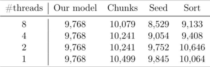
Table 2.1: Reproducibility evaluation :: Number of messages

#threads Our model Chunks Seed Sort

8 9,768 10,079 8,529 9,133

4 9,768 10,241 9,054 9,408

2 9,768 10,241 9,752 10,646 1 9,768 10,499 9,845 10,064

Table 2.1 presents the numbers of messages during the same simulated scenario, varying only the number of threads. We observed that when the simulated elements are created and allocated, specifically, into different numbers of chunks, the number of messages varies because the ordering of communication events is affected. For instance, the DSR algorithm generates more or fewer messages to discover an appropriate route because the order of messages arriving at a specific node could change in different simulations.

Table 2.2: Reproducibility evaluation :: Mobility events

8 1,505,846 1,504,906 1,508,174 1,512,714 4 1,505,846 1,488,315 1,487,004 1,503,054 2 1,505,846 1,488,315 1,457,107 1,472,960 1 1,505,846 1,492,151 1,525,011 1,513,041

(23)

2. Reproducibility in Parallel Sensor Network Simulations ₁₀

when using only one seed to generate the random numbers, the number of mobility events varies. This occurs because the event id, which is randomly generated, is not the same in all simulations; consequently, the event order used during the scheduling is not the same.

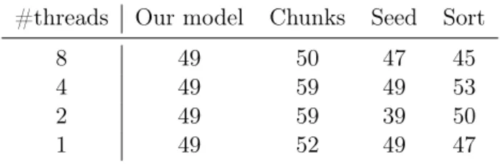
Table 2.3: Reproducibility evaluation :: Node deactivation

8 49 50 47 45

4 49 59 49 53

2 49 59 39 50

1 49 52 49 47

Finally, Table 2.3 illustrates the results on the number of node deactivations because this behavior is mandatory in several simulations. In our example, the environmental event lightning deactivates gateway sensors for a short period. We observed a difference in event ordering in different simulations when the synchronization mechanism is active but the sorting is not. These results demonstrated that sorting must work together with the synchronization strategy to achieve parallel reproducibility. The justification, as mentioned above, is the non-determinism of the OS threads. Specifically, the event order is not the same in different simulations; consequently, the event sequence in the environment cells does not follow the same order.

2.6 Conclusion

We presented a reproducible parallel simulation model to be adopted in sensor network sce-narios. Our model consists of wrapping all simulation elements into several chunks. All computations and communications of a simulation are performed from a single seed value and a pseudo-aleatory number generator. Consequently, it is possible to run chunks in parallel and to guarantee that each chunk can repeat its execution.

(24)

Chapter 3

JSensor: A Parallel Simulator for

Huge Wireless Sensor Network

Simulations

3.1 Abstract

This work presentsJSensor, a parallel general purpose simulator which enables huge simula-tions of wireless sensor networks (WSNs) applicasimula-tions. Its main advantages are: i) to have a simple API with few classes to be extended, allowing easy prototyping and validation of WSNs applications and protocols; ii) to enable transparent and reproducible simulations, regardless the number of threads of the parallel kernel; and iii) to scale over multi-core computer archi-tectures, allowing more the simulation of more realistic elements, such as the environment and application-events representing natural phenomena. JSensor is a parallel event drive simula-tor which executes according to event timers, so the simulation elements (nodes, application or events) can send messages, process task or move around the environment. The mentioned environment follows a grid structure of extensible spatial cells. The results demonstrated that JSensor scales well, precisely it achieved a speedup of 7.45 with 16 threads in a machine with 16 cores (eight physical and eight virtual cores), and comparative evaluations versus OMNeT++ showed that the presented solution could be 21% faster.

3.2 Introduction

The world around us has a variety of phenomena described by variables such as temperature, pressure, and humidity, which can be monitored by devices capable of sensing, actuating, pro-cessing, communicating and moving around the environments. Such devices, working cooper-atively, are termed wireless sensor networks (WSNs) Akyildiz et al. (2002a). WSNs simulators

(25)

3. JSensor: A Parallel Simulator for Huge Wireless Sensor Network

Simulations ₁₂

for large applications Chen et al. (2005), where thousands or even millions of nodes are simu-lated, are becoming regular with the advance of new WSNs applications, e.g., general Internet of things (IoT) applications Muruganandam et al. (2018), smart cities Lu et al. (2017), social sensing Ali et al. (2011) or natural environment monitoring Lin et al. (2015).

It is not simple to perform simulations of large WSNs applications, neither to achieve good speedup when we use parallel strategies for high-performance computing (HPC) architectures. The new WSNs applications have demanded robust simulators, e.g., simulators capable of evaluating scenarios with millions of nodes with protocols and speciﬁc models implemented. For instance, to simulate human behavior during one week in Tokyo downtown, based on cell phone information, would require millions of nodes with diﬀerent communication protocols and interference models Xiong et al. (2016).

Standards and market-leaders simulators, such as OMNeT++, NS, and others Varga and Hornig (2008b); Xue et al. (2007); Zeng et al. (1998a); Ould-Ahmed-Vall et al. (2007a), do not implement environment modeling and application-events to simulate interference from external agents or natural phenomena, such as rain, sun, lightning, and so forth, in Earth regions. Sundresh et al. Sundresh et al. (2004) detail the importance to model the complete application environment in a WSN simulation. They propose a model for indoor and outdoor environments made of tiles. Based on this simulator, it is possible to implement concrete, grass and walls tiles, each one with diﬀerent signal interference and propagation. However, the most simulators, in special HPC ones, do not consider this modeling.

Another limitation in WSN simulator is the non-reproducibility. In general, the users diminishes the reproducibility problem while implementing their simulation models in the simulators. Parallel simulations impose an extra challenge regarding reproducibility because they introduce the concurrency principle when implementing threads or processes sharing common resources, thus generating non-deterministic behaviors. In this case, repeatable par-allel simulations must treat the non-determinism. In summary, reproducibility can become very complicated in parallel scenarios, being not suitable to be designed by users.

(26)

Simulations ₁₃

To evaluateJSensor, we tested it with three diﬀerent applications: i) a robust data prop-agation application using the ﬂooding model; ii) a mobile phone application with communica-tion interference and WSN routing protocols; and iii) a sophisticated air quality applicacommunica-tion regarding CO2. We execute the experiments in two machines, one with 16 cores and other

with 24 cores, both with hythreading technology (50% of all cores are virtual). The per-formance results achieved speedups of 7.45 with 16 threads running concurrently. The com-parative evaluations of JSensor versus OMNeT++ reveled a runtime 21% faster of JSensor when simulating the ﬂooding model.

The remainder of this chapter is as follows: Section 3.3 discusses JSensor related work, pointing out their beneﬁts and limitations. Section 3.4 presents the JSensor kernel and its speciﬁcities. Section 3.5 explains the parallelism implementation adopted by JSensor. Sec-tion 3.6 shows theJSensor strategies that allow the reproducibility of parallel and large WSNs applications. Section 3.7 describes the applications used to test the simulator speedup and memory consumption. Section 3.8 presents the performance evaluations conducted and the results obtained. Finally, Section 3.10 concludes the chapter and presents some the future research directions.

3.3 Related Work

We evaluate several parallel simulators used to assess WSNs applications. Several surveys described diﬀerent WSNs simulators, their limitations, and their improvements Weingärtner et al. (2009); Khan et al. (2011); Chhimwal et al. (2013b); Sundani et al. (2011b); Yick et al. (2008); Akyildiz et al. (2002b); Vieira et al. (2003); Yu and Jain (2011); Minakov et al. (2016). In general, a WSN application presented the following elements: i) manager interfaces, e.g., data visualization or node range controllers; ii) high level distributed algorithms, e.g., clus-tering, localization, or data aggregation strategies; and iii) low-level protocols, e.g., routing, duty cycle, or address naming protocols. Normally, the simulators are used to evaluate high level distributed algorithms Barr et al. (2005b); Distributed Computing Group (2015) or low level protocols Zeng et al. (1998a); Doerel (2009); Riley and Park (2004b); Ould-Ahmed-Vall et al. (2007a). In both cases, it is possible to simulate a complete WSN application.

(27)

Simulations ₁₄

some application-events can occupy vast regions of Earth, like wind or sun, thus many cells of the environment, but a node always holds a single cell per simulation time; vii. The simulator project artifacts, e.g., programming and installation guides for users, discussion lists, if the solution is open source or not, discontinued or active, free or commercial and many other project issues.

To the best of our knowledge, Java in Simulation Time (JiST) Barr et al. (2005b) is the unique parallel simulator specialized in high level distributed algorithms. It is based on discrete events and could be used combined with Scalable Wireless Ad hoc Network Simulator (SWANS) Liu et al. (2001). In this simulator, each network element is an entity that can create events to be simulated. It performs the interactions among entities after synchronization barriers. Out of synchronization barriers, entities are independent, allowing the simulator do scale up regardless the application domain. JiST meets the “Multi-core support” and “Project artifacts” features.

On the other hand, we found several parallel simulators specialized in low-level protocols. One of them is the Global Mobile System Simulator - GloMoSim Zeng et al. (1998a), which is designed with libraries for WSN simulations. It is based on parallel discrete events and uses a C-like parallel simulation language (PARSEC) Bagrodia et al. (1998). There is a set of modules where each of them simulates a speciﬁc network protocol in the communication stack. There are a large number of protocols available in the GloMoSim library. To minimize the overhead of large-scale WSNs simulations each kernel thread is responsible for simulating one layer of the communication protocol stack. GloMoSim meets the “Multi-core support” and “Network protocols” features.

TheGloMoSim commercial version is the Qualnet Doerel (2009). It was released in 2000 by Scalable Network Technology (SNT)1_{. Some additional features in the commercial version}

are a GUI based simulation, high ﬁdelity commercial protocols and device models, comparative performance evaluation of alternative protocols at each layer, built-in measurement on each layer, modular layer stack design, and support for multiple parallel simulation strategies. Qualnetmeets the “Multi-core support”, “Network protocols”, and “Project artifacts” features. A widely used simulator for WSNs application is Castalia. Castalia is based on the OM-NeT++ platform Varga and Hornig (2008b) and can be used to test distributed algorithms or protocols in realistic wireless channel and radio models. It also implements MAC and routing protocols. It is necessary to integrate MPI in OMNeT++ platform to perform parallel simula-tions. Therefore, it becomes diﬃcult for users without HPC skills. Another drawback in using MPI over multicore computer architectures is that most of its implementations are for multi-computer clusters with private memory abstractions. Therefore, network communications are considered even in a shared memory multicore architecture what introduces a considerable overhead. Castalia meets the “Network protocols” and “Project artifacts” features.

(28)

Simulations ₁₅

Other parallel simulator, based on Network Simulator version 2 (NS-2) Xue et al. (2007), is theParallel Distributed NS (PDNS) Riley and Park (2004b). It uses a conservative, blocking based, an approach for synchronization with a possible sub-optimal speedup. It inherits all protocols, models, and applications of NS-2. However, all complexity and program diﬃculties are inherited too. Vodel et al. Vodel et al. (2008) mention that “the integration with such a complex framework, like NS-2, constrains PDNS to several conceptual limitations”. PDNS meets the “Multi-core support”, “Multi-computer support”, and “Network protocols” features. The NS-3 Riley and Henderson (2010) is also a version of the NS family, which is intended to replace the predecessor, NS-2. It has a discrete-event simulation engine written in C++ and a modular object-oriented architecture. The NS-3 provides a range of traditional protocols, such as TCP/IP, IPv6, and IEEE802.11. The simulator supports parallel and distributed simulation using MPI. Another novelty is the possibility of using Python in conjunction with C++ in some parts of the simulation. NS-3 meets the “Multi-core support”, “Multi-computer support”, “Network protocols” and “Project artifacts” features.

Finally, we found the Georgia Tech Sensor Network Simulator (GTSNetS) Ould-Ahmed-Vall et al. (2007a). It allows the development and evaluation of algorithms for large-scale WSNs. GTSNetS is complete, providing diﬀerent energy models, battery models, network protocols, application protocols, and tracing options. Furthermore, the users could easily extend or replace the available models for a speciﬁc requirement. GTSNetS reports that could handle 200 thousand nodes in a simulation Khan et al. (2011). GTSNetS meets the “Network protocols” and “Project artifacts” features.

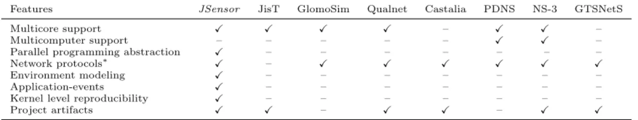
A summary of presented features among cited works andJSensor is presented in Table 3.1. As observed, JSensor meets most of the presented features.

Table 3.1: Summary of related work features

Features JSensor JisT GlomoSim Qualnet Castalia PDNS NS-3 GTSNetS

Multicore support X X X X – X X –

Multicomputer support – – – – – X X –

Parallel programming abstraction X – – – – – – –

Network protocols∗ X – X X X X X X

Environment modeling X – – – – – – –

Application-events X – – – – – – –

Kernel level reproducibility X – – – – – – –

Project artifacts X X – X X – X X

∗_JSensor_{considers only the routing layer}

(29)

Simulations ₁₆

often in a simulation, it is necessary to change the environment, so this simulation element must be extensible and dynamic. Diﬀerent of presented simulators, JSensor implements a thread-safe environment to simulate vast territories of Earth. To discretize continuous Earth regions, JSensor adopts a grid of cells with extensible properties, very similar to a raster representation of Geographic Information Systems (GIS).

3.4 JSensor

_{Parallel Simulator}

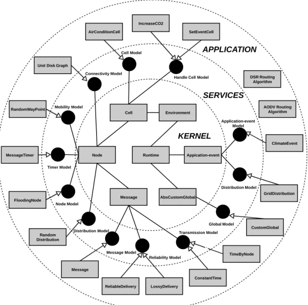
JSensor is coded in Java, which means it is portable to many platforms with a JVM running. It is designed to execute asynchronous simulations based on events. Its architecture, illustrated in Figure 3.1, is organized into rings, according to its behaviors and visibility to users.

Runtime Appication-event Node Message Environment Cell AbsCustomGlobal KERNEL Global Model CustomGlobal Node Model Mobility Model Distribution Model Connectivity Model Message Model Reliability Model Transmission Model Handle Cell Model Cell Model Application-event Model Distribution Model Timer Model GridDistribution ClimateEvent MessageTimer RandomWayPoint FloodingNode Random Distribution Message ReliableDelivery ConstantTime Unit Disk Graph

AirConditionCell IncreaseCO2 SERVICES APPLICATION DSR Routing Algorithm AODV Routing Algorithm LossyDelivery TimeByNode ' SetEventCell

(30)

Simulations ₁₇

The more outer rings abstractions can adopt any inner ones so that the elements of the n-th circle can inherit behaviors from any inside ones. The most internal ring represents the kernel, where fundamental concepts are responsible for running simulations. The service layer provides diﬀerent features for users develop their models and applications. Finally, the application layer represents the simulated application, each feature inJSensor has a practical example from an already developed model as illustrated in application ring on Figure 3.1.

3.4.1 Kernel Layer

The kernel layer creates the threads for parallel events execution, the chunks to guarantee reproducible parallel simulations with a diﬀerent number of threads (detailed in Section 3.6), the environment which encapsulates a grid of cells, and the capability to log the simulation data. Furthermore, the kernel executes send-receive, timer, mobility and other simulation events of nodes and application-events. All simulation events have a predeﬁned time to occur and JSensor guarantees their order by considering their internal clocks. Regularly, JSensor removes and executes events according to a global clock.

The kernel layer is composed by:

• Runtime: It is the main class, responsible for managing the structure of the kernel. It contains the lists of nodes and application-events, the chunks, and the environment. Furthermore, this class controls the threads that execute the simulation models, and it keeps the simulation times synchronized.

• Node: It represents the general node in a WSN application. Any new node type must extend the class Node. Nodes can have a variety of sensors, and they can move through the environment, interact with the environment, have an initial position, identify their neighbors, execute speciﬁc events, and communicate with other nodes. The communi-cations are send-receive message events, classiﬁed in two types: Unicast and Multicast.

• Message: It is responsible for performing the communication between nodes. Using the Unicast or Multicast methods of the nodes, the message will be sent according to protocols, delays, package losses, channel noises, and any possible interference deﬁned by the user. All new application messages must be a specialization of this class. Thus, it must implement a clone()method to enable copies of itself.

• Application-event: It represents an application phenomenon, natural or not, with life-time, topology, mobility, and capacity of interacting with the environment. We observe the entire interleaving of events and nodes, e.g., when environmental changes occur, made by application-events, the nodes can perceive them.

(31)

Simulations ₁₈

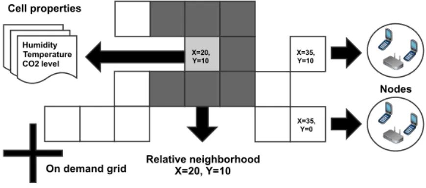
read and write cell properties from regions where they live, concurrently and in a thread-safe manner. The Figure 3.2 illustrates that multiple nodes, application-events or their combinations are in a cell. They can read its properties and write new values into it, so the concurrent write operations are synchronized transparently by the kernel.

X=35, Y=10

X=35, Y=0

Nodes

X=20, Y=10

Relative neighborhood X=20, Y=10

Humidity Temperature CO2 level

Cell properties

On demand grid

Figure 3.2: Grid of cells.

Despite the fact that the modification of a single cell is sequential, the cell modification step executes in parallel by splitting the cells into chunks, so all changes for a specific cell are made by the same chunk and, consequently, the same thread. The chunk concept and its benefits will be explained in details in Section 3.5.

• Environment: It is a map of spatial cells where the user can build his cells to customize the environment. A cell exists only if a node or an application-event have inhabited or modiﬁed it, in this way we build the JSensor environment on-demand. This process is essential for a simulator designed for large-scale scenarios, for instance, over vast territories of the Earth.

• AbsCustomGlobal: It maintains and controls general simulation timers. Besides, it en-ables the user to ﬁnalize the simulation and perform actions at key points, precisely before and after the execution of each simulation round and after the complete simula-tion.

3.4.2 Services Layer

JSensor provides a set of services for users so that they can develop their models for nodes, messages, cells, or application-events. To implement a new model, the users must extend JSensor existing types or implement diﬀerent interface classes.

(32)

Simulations ₁₉

to check the messages received in a speciﬁc event and to process them according to their needs.

• Distribution Model: The unique method of this interface isgetPosition(Node n), used to distribute the nodes through the environment during the initial state of the simulation, i.e., during the simulation ﬁrst event. The method has a node as the argument and must return a valid position for this node.

• Connectivity Model: It represents the nodes interconnections. There are two types of connection between nodes, logical and physical. The logical one deﬁnes if a pair of nodes can communicate and its implementation is through the methodisConnected(Node from, Node to), which requires two nodes as arguments and returns a boolean value. The physical one occurs if two nodes are near enough to receive signals from each other and its implementation is through the methodisNear(Node n1, Node n2), requiring two nodes

as arguments and returning a boolean value.

• Message Model: This interface allows users to create messages according to their needs. For that, it is necessary to implement the clone() method so that the kernel can create copies of the messages.

• Timer Model: Timers create new simulation events, allowing the simulation to schedule a task in the future.

• Reliability Model: It abstracts the reliability of the simulated network. For each mes-sage, the model decides if it should arrive at the destination or not. For several reasons a network packet cannot reach the destination, so JSensor enables such scenarios via reliability model implementations. The unique method necessary to build a new relia-bility model is the reachesDestination(Message msg) method, which returns a boolean value that indicates if the simulation should drop the message.

• Transmission Model: The message transmission model deﬁnes how much time the mes-sage spent until it reaches the destination. The method timeToReach(Node nodeSource, Node nodeDestination, Message msg) needs to be implemented and it returns a ﬂoat value that represents the time.

(33)

application-3. JSensor: A Parallel Simulator for Huge Wireless Sensor Network

Simulations ₂₀

events change cells concurrently, even in non-commutative simulations, assuring the reproducibility.

• Distribution Model: By using this interface, the user can implement a distribution model for the application-events. The method getPosition(Event e) must be imple-mented and it returns a valid position for the application-event e.

• Cell Model: The users can create cell models according to their needs. The unique method to be implemented is the clone() method, which is adopted by the kernel to create copies of the cells to perform safe modiﬁcations.

• Handle Cell Model: The application of this model changes cells, keeping the consis-tency of the simulation state and also the reproducibility since the simulator must replace the cells in the same order, regardless it is an aleatory order or not. Due to JSensor’s parallel characteristic, the user must implement a handle model to keep the right or-der. The method to be executed is the fire(Node node, CellModel cell), which has as arguments the node associated with a cell and the changed cell.

• Mobility Model: It deﬁnes how the nodes will move during the simulation, so to develop a new model the user must implement the methodsgetNextPosition(Node n)andclone(). The ﬁrst one must return a valid position for the node n and the clone is adopted by the kernel to create copies of the model to perform parallel executions safely.

• Global Model: This model encapsulates several useful JSensor features. The method hasTerminated() stops the simulation when it returns true. Furthermore, it has the methods preRun() and postRun(), which are executed before and after the simulation, respectively. In the same context, the methods preRound() and postRound() can be executed before and after each round. A round represents a complete cycle of steps, e.g., move, send a message and discover neighbors. Each of these steps can have zero or more events to be simulated.

3.4.3 Application Layer

JSensor implements different applications to offer a significant number of features for new users. The following features are available in JSensor through the Flooding, Mobile Phone, and Air Quality applications detailed on Section 3.7.

(34)

Simulations ₂₁

• The Flooding application implements the RandomDistributionmodel, which generates pseudo-random numbers to deﬁne the position of the nodes.

• The default connectivity implementation onJSensor is theUnitDiskGraphconnectivity, which connects the nodes if they are inside each other’s radius. The ﬂooding applica-tion connects all the nodes in the logic level, and it does not deﬁne a new physical communication, letting JSensor to use the default UnitDiskGraphmodel.

• The Flooding application implements a simple Message that contains the sender and destination nodes, the message to be transmitted and a counter to hold how many hops the message had until the destination. In this case, a message containing sender ID, destination ID, a counter for the number of hops and the message content.

• The ﬂooding application adopts a timer to send the initial messages (MessageTime). At the methodfire() of the timer, the simulation sends the message to all neighbors of the node via broadcast. To start the timer, its method startRelative() is called, passing as argument a time and a node.

• The Flooding application adopts the ReliableDelivery model, which does not drop any message.

There is also the LossyDelivery model in JSensor, which drops 5% of messages ran-domly.

• The Flooding application adopts ConstantTime transmission model, which returns a constant time.

JSensor has also the TimeByNode transmission model, which returns a value based on the type of node sending the message.

• JSensor has the ClimateEvent model used by the Mobile Phone simulation to change the climate according to previously deﬁned states, precisely sunny, cloudy, rainy and rainy with lightning.

• On Mobile Phone application, the climate event is distributed in grid implemented by

GridDistribution model, so it covers all the environment.

• The Air Quality application uses a Cell Model with CO2 level, water level, and a

boolean value for lightning presence through the AirConditionCell model. The CO2

levels indicate the amount of gas in a cell. The water level means the water accumulated by several hours of rain. The lightning indicates if it struck a cell recently.

(35)

Simulations ₂₂

• The Air Quality application uses theIncreaseCO2model to increase the CO2 level based on the node that produced it.

• JSensor has Random Way Point mobility model to guarantee that a node will move in one of eight possible positions selected randomly or will stay in the same place an aleatory time. The user in the simulator can also deﬁne the distance traveled by the nodes in each movement. All applications implemented use the Random Way Pointmodel.

• All simulations use the CustomGlobal implementation. This class is especially useful for debugging and obtaining global simulator information, so, for instance, we can use JSensor’s logging ﬁles at the end of each round to write which cells had CO2 level above

a threshold, using the postRound()method. The simulation uses the method postRun() when it ﬁnishes, for example, to write the ﬁnal values of the CO2 level from each cell.

Besides the above implementations,JSensor provides two fundamental routing algorithms: DSR Johnson et al. (2001) and AODV Perkins et al. (2003). The simulation could straight-forwardly integrate these algorithms. We use these routing algorithms in the Mobile phone and Air quality applications.

3.5 JSensor

_{Parallel Kernel}

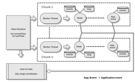
JSensor simulates nodes and application-events in parallel over multicore HPC architectures, as illustrated by Figure 3.3. The Runtime class, introduced previously, manages a pool of worker threads, where each worker is responsible for one or more chunks. As depicted on Fig-ure 3.3, each chunk contains the respective set of nodes and application-events. In summary, there are w workers active in a machine with w cores and each worker has a similar number of chunks and nodes to simulate.

The nodes share a grid of cells, named environment, and eachJSensor cell has coordinates latitude-longitude and which nodes exist in the cell. Cells exist only if there is at least one node dwelling it or if an application-event has modiﬁed it. As shown in Figure 3.3, the worker threads and, consequently, the nodes access the grid to change properties of the environment, so for concurrence reason, the grid needs to be thread-safe.

The size of the cells to build the grid can be varied. Thus the grid size parameter impacts the runtime of the simulations since the simulator needs to reach more cells to deﬁne the neighborhoods of a node when cells size is small. We identify the same eﬀect when we use large communication ranges in the node.

(36)

Simulations ₂₃

Class Runtime

int currentTime int nextTime

Worker Thread Node

msg

App. event

Worker Thread Node

events msg

App. event

Grid of Cells

(lat, long) coordinates

events events

events

App.?event = Application-event

Chunk 1

Chunk n

Figure 3.3: Parallelism in JSensor

that are entirely within the communication radius because the nodes that belong to them are neighbors. However, there are several partially covered cells, and therefore all nodes inside these cells should be checked to determine whether or not they are neighbors.

Figure 3.4: Cell size inﬂuence.

As observed, more cells to be verified increase the runtime and the optimal cell size is a value near the communication radius of the nodes, as illustrated in Figure 3.4 by the second grid example, where the cell size and the communication radius are both 300 meters. The third scenario illustrates an example where the communication radius is 300 meters, and the cell size is 600 meters. In this case, once the cell size is bigger than the communication radius, the environment will have fewer cells. Although there are fewer cells to be verified, the number of nodes in each cell is significant, including also nodes far away from the communication radius of the node under evaluation.

(37)

Simulations ₂₄

the cells, just changing the position of the nodes. If the node moves to another cell,JSensor creates a new one if it does not exist, due to on-demand creation strategy explained before, and then move the node. As a parallel kernel, several worker threads can be moving nodes to the same cells, so JSensor needs to ensure synchronization. Each worker thread blocks the cell until it ﬁnishes the write operations. The synchronization order to access a shared simulation resource, e.g., a cell or a node message inbox follow a predeﬁned rule to achieve both performance and reproducibility, explained in details in the next section.

A signiﬁcant capability is the synchronization strategy on JSensor. To perform the syn-chronization the classRuntime is responsible for maintaining events ordered according to its internal clock. JSensor creates synchronization barriers after the simulation of a new set of nodes in speciﬁc event time, so it assumes that there are nodes simulating events at the same time. Thus, they can execute in parallel without interference. It is important to make it clear that JSensor works with a bag-of-tasks style parallelization, where the elements of the simulation are split between the chunks to run in parallel.

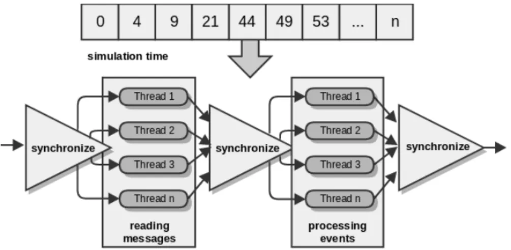
JSensor goes further, detailing what execution means, so internally it enables a node to communicate, calculate its new neighbors, sense the environment, move through the simulated environment and so forth. This way,JSensor implements synchronization barriers, figure 3.5, after each simulation step finishes, i.e., after mobility, connectivity, send-receive message and sensing simulation steps, for instance. We simulate in parallel nodes operating at the same time and doing the same event type (e.g., sending a message), so it is possible to affirm that inJSensor there are no nodes in parallel at same simulation time and on different simulation steps. We adopt the same assumptions for application-events.

Figure 3.5: Synchronization barriers

(38)

Simulations ₂₅

position are often ineﬃcient since nodes are not distributed uniformly in the environment once they move in the simulated area, changing their locations during the simulation. The partition of workload using protocol stack layers, provided in Zeng et al. (1998a); Doerel (2009) simulators, cannot scale for large number of threads, requiring a second task partition strategy.

Finally, the Algorithm 1 presents the core logic of Runtime class. It has access to all elements of the simulation, including current_time, the list of nodesN, the list of eventsE, and the shared grid in which the nodes reside G. The list of nodesN consists of k sublists, wherekis the number of machine’s cores. The same is true for the list of application-eventsE. This way, each sub-listN kandEkis associated to a chunk. This partition schema into chunks is required to guarantee that each thread simulates its respective nodes and application-events, avoiding concurrent accesses and, consequently, bottlenecks.

Algorithm 1Runtime main execution Require: time,N,E,G

1: whilet≤timedo

2: _for i←0. . .|σ|_do

3: _forj←0. . . k _do

4: events←Hold the list of events will execute at time t

5: Performs theevents of the stateσ_i of all nodes

6: events←Hold the list of events to be executed at time t

7: Performs theevents of the stateσ_i 8: _{end for}

9: Synchronize allN who performedσ_i 10: end for

11: _{end while}

Analyzing the Algorithm 1 we have:

• Line 1: Loop deﬁnition to execute each simulation time t.

• Line 2: Loop deﬁnition to execute all simulation steps σ. The steps are partitioned according to actions of the simulator, such as: σ1 mobility, σ2 connectivity, σ3 message

send-receive,σ4 sensing, and σ5 general-purpose computing events.

• Line 3: Loop deﬁnition to execute all kthreads. In eachσ step the simulator starts all

k threads of the simulation with their list of nodes and application-events, executing all events that have compatible time. More speciﬁcally, we implemented a thread pool to avoid the creation and destruction of threads repeatedly, thus maintaining some threads active while the simulation occurs.

(39)

Simulations ₂₆

execution. This strategy ensures that nodes or application-events can move, connect, send-receive messages and create new events in parallel, however, one step at the time.

3.6 JSensor

_{Reproducibility}

Parallelism affects both simulations causality, creating changes over events dependents, as the numerical reproducibility. The events can be simulated in a different order during different runs of the same simulation because of the non-reproducibility of communication between processors. The change in the order of only two events of a simulation may end up generating entirely different results. As detailed in Cleveland et al. (2013b), the change of event simulation order can lead to numerical inconsistency, caused by changing the order of double precision floating operations. This problem occurs not only with mathematical operations but in any simulation that deals with non-commutative operations.

As a simulator, JSensor must allow the reproducibility of simulations. In Dalle (2012b), the authors detail types of reproducibility, as well as simulations examples and reproducibility requirements. There are four levels of reproducibility, level one is the most restricted and used by JSensor. Level one is also known as the repeatability property; it designates the ability to re-execute the same simulation history as previously regarding computation, including the in-herently non-deterministic computations. In the case of discrete-event simulation, for example, repeatability means that the simulations produce the same series of events and process them in the same order. In the case of distributed simulations, in particular, repeatability implies that parallel activities, e.g., when the event occurs at the same simulation time, the processing must always be in the same order, which requires some additional synchronization Fujimoto (2000).

Reproducibility of sequential simulations is trivial because they need a seed and a good random number generator. In this way, we ensure the same sequence of numbers from the seed as often as necessary. In case of parallel simulators, the reproducibility is not trivial, since multiple threads or processes execute concurrently and often nodes are simulated without any synchronization. JSensor has reproducibility level one of the sequential and parallel simula-tions, regardless the hardware used or the number of threads started to perform the simulation. A simulation can contain non-deterministic models, arising from the use of pseudo-random numbers as alternatives for deﬁning probabilities. Algorithms for mobility, communication, the initial distribution of nodes and many more frequently use pseudo-random numbers.

(40)

Simulations ₂₇

cores to deﬁne the number of chunks,JSensor allows the user to start it with worker thread pool equals or less than the number of machine cores, so it ensures reproducibility of simula-tions with the same amount of threads or not. In summary, we adopt the highest concurrency level to deﬁne the number of chunks, since each worker thread must manage at least one. This way, all other concurrence level adopted in the same machine or not will be smaller and repeatable by JSensor.

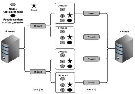
As explained above, each worker thread simulates a set of nodes and application-events. Therefore, each thread can simulate one or more chunks of nodes and application-events. The chunks are never shared among threads to avoid unnecessary synchronizations. The idea to start from only one seed and to generate other seeds based on the number of chunks enables reproducibility in parallel since now each chunk with several nodes and application-events have their seeds to repeat in other executions. Each chunk has a seed and a random pseudo-numbers generator, regardless the number of threads on execution. Non-proportional pseudo-numbers to deﬁne both the number of worker threads and the number of chunks, e.g., four workers and seven chunks, in a simulation can allocate more chunks to one worker thread than others, so they should be avoided.

Figure 3.6 illustrates a machine with four processing cores and how it is possible to compare the same simulations running with two threads and then with four worker threads. Initially, the nodes are partitioned into four chunks, regardless of the number of threads the user selected in the simulation. In Figure 3.6 (a), the user chooses two threads. Thus, each thread will simulate the nodes and application-events of two chunks sequentially. In the Figure 3.6 (b), we have four threads, so each thread simulates the nodes and the application-events of a single chunk. The JSensor simulates nodes and application-events of a chunk in the same order, and we guarantee the same sequence of pseudo-random numbers from a seed and a generator since each chunk is a sequential simulation. Thus, as shown in Figure 3.6, no matter the number of worker threads, each thread JSensor always simulate the same nodes and application-events in the same order. The unique restriction is that the number of chunks requires being higher or equal than the number of worker threads.