adfa, p. 1, 2011.
© Springer-Verlag Berlin Heidelberg 2011
Forecasting of a Non-Seasonal Tourism Time Series with
ANN
Teixeira, João Paulo1 & Fernandes, Paula Odete1,2
1Polytechnic Institute of Bragança; UNIAG 2NECE
[email protected]; [email protected]
Abstract. The paper present and discusses several alternative architectures of Artificial Neural Network models used to predict the time series of tourism de-mand for Cape Verde. This time series is particularly difficult to predict due to its non-seasonal characteristic usual in a similar time series for European Tour-ism destinations. The time index used as input and other input parameters varia-tions improved the performance of the prediction over the test set to a relative error of 7.3% and a Pearson correlation coefficient of 0.92.
Keywords: ANN; Forecast; Non-seasonal time series; Tourism; Cape Verde.
1
Introduction
Modelling and forecasting tourism demand has received in the last decade’s a sub-stantial attention among researchers, policy makers, hospitality management, and other interest groups. Forecasting tourism demand being a significant activity for its beneficiaries and stakeholders’, several forecasting models have been applied to esti-mate and forecast the tourism demand.
methods have also been implemented in tourism forecasting. The most commonly used AI methods are artificial neural network (ANN) models (Kon & Turner, 2005; Palmer et al., 2006; Fernandes et al., 2008; Fernandes et al., 2013). But, according to Song and Li (2008) there is no one model that stands out in terms of forecasting accu-racy. Therefore academics and practitioners continue to improve and develop models and methods to bring about greater understanding of the economics and business principles as guidance for more effective management and planning in the tourism sector.
In this way, with this paper it is intended to present and discuss several alternative architectures of Artificial Neural Network models used to predict the time series of tourism demand for Cape Verde. For that it will be used the time series “Monthly Guest Nights in Hotels in Cape Verde” registered between the period January 2005 and December 2011, and collected by National Statistics Office of Cape Verde (INECV, 2013). It is one of the most used time series in the academic and scientific field, to describe the tourism demand.
The remaining sections of this paper are organized as follows: After this introduc-tion; in section 2 the time series “Monthly Guest Nights in Hotels in Cape Verde” is presented and analysed; Artificial Neural Network models will be presented in section 3; the empirical results are given in section 4. A concluding discussion finishes the paper.
2
Tourism Demand Time Series of Cape Verde
The archipelago of Cape Verde is made up of ten volcanic islands (Santo Antão, São Vicente, Santa Luzia, São Nicolau, Sal, Boavista, Maio, Santiago, Fogo and Brava) and eight islets which make up a total area of 4033 km² (PEDTCV, 2010). There has been an exponential increase in the number of overnight stays which, in 2000, totalled 685 thousand and in 2012 already exceeded 3 million (INECV, 2013). Over this period the average annual increase in overnight stays in hotel establishments in the country was around to 14%, while, last year, the number increased by 17.9% in relation to 2011 (INECV, 2013). There continues to be strong reliance on foreign tourism – over 95% of overnight stays – almost exclusively represented by European markets. The most important markets in 2012 were: the United Kingdom, 31.7%; Germany, 14.9%; Portugal, 9.5%; and France, 9.0%. The islands of Boavista and Sal stand out clearly as being the destinations most capable of attracting tourists, repre-senting 90% of overnight stays; 47.4% on the island of Boavista and 42.2% on the island of Sal (INECV, 2013).
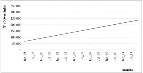
Fig. 1. Monthly Gu
Is possible to see clearl when compared with othe trend. However, it is note month of December presen
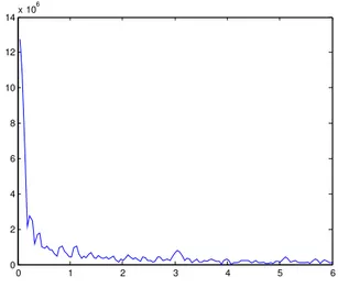
An analysis using the F The Fourier transform was responds to one month, the fore the 256 sample of Fo the first 128 samples (cor scaled to 6. This means t quency of half of Fs/2, me that is usual to find 3 pea month long in this time ser
0 50,000 100,000 150,000 200,000 250,000 300,000 350,000 Ja n _ 0 5 Ju l_ 0 5 Ja n _ 0 6 N º o f O v er n ig h ts
Guest Nights in the Cape Verde, from 2005:01 to 2011:12.
arly the non-seasonality of the time series, that is no comm ther tourism demand time series, along with a clear upwa oteworthy that the month of August and in some years sents the highest peaks.
e Fourier transform of the time series is presented in Fig. as performed with a length N of 256. Since each sample c the sampling frequency Fs is the inverse of one month. The Fourier transform corresponds to Fs frequency. In Fig. 1 on
orresponding to Fs/2) of Fourier transform is presented a s that the visible peak that appears at 3, corresponds to f
eaning Fs/4 that is the inverse of 4 months. This correspon eaks per year or that there are a repetition of periods with series. Ju l_ 0 6 Ja n _ 0 7 Ju l_ 0 7 Ja n _ 0 8 Ju l_ 0 8 Ja n _ 0 9 Ju l_ 0 9 Ja n _ 1 0 Ju l_ 1 0 Ja n _ 1 1 Ju l_ 1 1 Months mon ward s the
Fig. 2. Fourier analysis of the time series.
3
Artificial Neural Network Models
Due to the non classical time series that makes difficult the forecasting of future values because non seasonal characteristics seem to be present in the time series sev-eral experimental architectures and input data will be used in models in order to evaluate the possibility of make predictions with some degree of confidence. The experimented ANN models already have been used to predict a similar tourism time series but for other country and/or region of country with good results. Anyhow it should be mention that all time series used in those models has the characteristic of seasonality.
All the ANN used has one output node to predict the value of the time series for next month but the model should predict the values for next twelve months. With the ANNs with one output the prediction for twelve month is made in 12 iterations of prediction using the output of previous iteration as input for next prediction.
The following 5 models and inputs have been experimented:
• Model A – consists in a feedforward architecture ANN with 12 input nodes one output node and 4, 6 and 8 nodes in the hidden layer. The input consists in the val-ues of the previous twelve months. The output is the forecast for next month. This model already has been used with success result for the time series of the North Region of Portugal (Fernandes et al., 2013).
• Model B – consists in a feedforward architecture ANN using the time index in its entrance. The ANN has 14 inputs, and one output and 4, 6 and 8 nodes in the hid-den layer. The time index is modelled in two variables one for the month and the other for the year. The month varies from 1 to 12 corresponding to the month of the year (1 – January ... 12 – December). The year varies from 1 for the values of
0 1 2 3 4 5 6
0 2 4 6 8 10 12 14
the first year (2005) until 7 for the last year (2011). This model already has proved its ability to forecast a similar time series with a strong rising tendency (Fernandes & Teixeira, 2009).
• Model C – consists in a feedforward architecture ANN using only the variable with the year in its entrance. This model is very similar to model B but discard the vari-able month because the time series seem to do not be sensitive to the month. Any-how the year is kept because of the rising tendency of the time series. The remain-ing inputs, output and hidden layer are the same as the ones of models B.
• Model D – consists also in a feedforward ANN using the year in its entrance but now using only the previous 5 months in the input. Therefore the model D ANN has 6 input nodes only and the remaining is similar as model C. This experiment intends to verify the importance or not of one year of data in the input.
• Model E – consists in a feedforward ANN similar as model B but using the time series in the logarithmic domain. This last model has used in order to verify if re-ducing the amplitude differences between months it could improve the forecast er-ror. The architecture and input features were the same as model B, because after a first analysis model B had lower forecast error.
The five ANN models had been experimented with different number of nodes in the hidden layer. Four, six and eight (4, 6 and 8) nodes were experimented for each model. The available data of the time series is relatively short to consider more nodes in the hidden layer, because it would increase the number of weights to be adjusted during training process. Considering, for instance the model A with 12 inputs, and M the number of hidden nodes, the total number of weight to be adjusted are 12*M+M*1. Additionally there are also the bias weights that are also M+1. For M=8 it gives 104 weight and 9 bias. Considering only 64 input/output pair it is too much weight parameters to be adjusted.
The data set was divided in a training, validation and test set. The test set was used for a final evaluation of the model performance and consists in the last 12 month, corresponding to the last year (2011). The validation set was used for a cross valida-tion process to early stop training. The set corresponds to the 12 months of the year 2010. The training set, used to train the ANN, corresponds to remaining data in a total of 60 months. Actually only 48 months were available to train for models A, B, C and E because the previous 12 months are need for the input. For model D 55 month were used for training because only 5 months are need for the input.
All the ANN models were trained with the Levenberg-Marquardt training function (Marquardt, 1963). The Resilient back propagation algorithm (Riedmiller & Braun, 1993) has also experimented but with worst results.
4
Discussion of Results and Models
The quality of prediction is measured by the ability of the model to fit the curve of target data. This ability is analysed by the MRE and by the Pearson Correlation coef-ficient (r) between target and predicted data set. The MRE measures the distance between target and predicted values of a given set. The correlation coefficient meas-ures the similarity between the two curves of the given set. It is possible to have a high similarity between the two curves (high r) but the curves can be very different in their absolute values. The correlation coefficient can evaluate the ability of the model to catch the variation along the months of the year and MRE can evaluate the ability of the model to follow the accurate amplitude of the time series.
Target data is the original values of the time series.
1
1 n
i i
i i
T P
MRE
n = T
−
=
∑
[1]with: Pi, Predicted value for month i and Ti, Target value for month i.
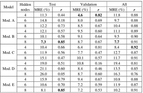
The MRE and correlation coefficient along test set, validation set and considering the all data for the 4 models using 4, 6 and 8 nodes in the hidden layer is presented in table 1.
The best models considering the all data set has model B with 8 nodes in hidden layer that reached the lower MRE (7.7%), and model C with 4 nodes in hidden layer that reached the higher r (0.92).
Considering the validation set clearly model A with 4 nodes in hidden layer achieved simultaneously lower MRE (4.6%) and higher r (0.82).
For the test set model C with 8 nodes in hidden layer has again the one with best result both considering MRE (7.3%) and r (0.85). Though model E with 8 nodes in hidden layer also reached the same r (0.85).
The result considering the All data set cannot be taken very seriously because most of the data were used in training process been used to adjust weights. Validation set was used during training process to stop train early and to select the best training ses-sion along 50 training sesses-sion. And data of the test set were not seen during training process. Therefore the model with better performance along this set should be consid-ered the selected one.
Table 1. Performance of models.
Model Hidden nodes
Test Validation All
MRE (%) r MRE (%) r MRE (%) r
Mod. A
4 11.3 0.44 4.6 0.82 11.8 0.88
6 14.8 0.18 8.0 0.69 9.7 0.88
8 12.2 0.73 8.5 0.67 10.4 0.88
Mod. B
4 12.1 0.57 9.5 0.60 11.1 0.89
6 10.1 0.58 9.1 0.64 9.5 0.90
8 7.3 0.85 8.7 0.67 7.7 0.91
Mod. C
4 10.4 0.66 6.4 0.81 8.4 0.92
6 11.9 0.56 7.7 0.47 12.7 0.87
8 15.1 0.47 10.1 0.57 11.7 0.91
Mod. D
4 19.0 0.51 10.8 0.16 19.4 0.81
6 21.1 0.60 8.4 0.46 13.5 0.85
8 26.0 0.05 8.7 0.60 16.3 0.76
Mod. E
4 15.9 0.79 9.4 0.67 10.8 0.88
6 10.6 0.70 7.2 0.59 11.9 0.87
8 8.1 0.85 7.2 0.53 10.2 0.91
Comparing the best results of the model B for this non-seasonal time series with the best performance of ANN for seasonal time series, this model reached a MRE of 7.3% against an MRE of level between 5.4% and 7.3 % using a model similar to model A in Fernandes et al. (2013) or 5.8% and 6.4% using models similar to present models B and A, respectively in Fernandes and Teixeira (2009). Considering the cor-relation coefficient r this model reach 0.85 in this non seasonal time-series against 0.98 in Fernandes et al. (2013) using a seasonal time series.
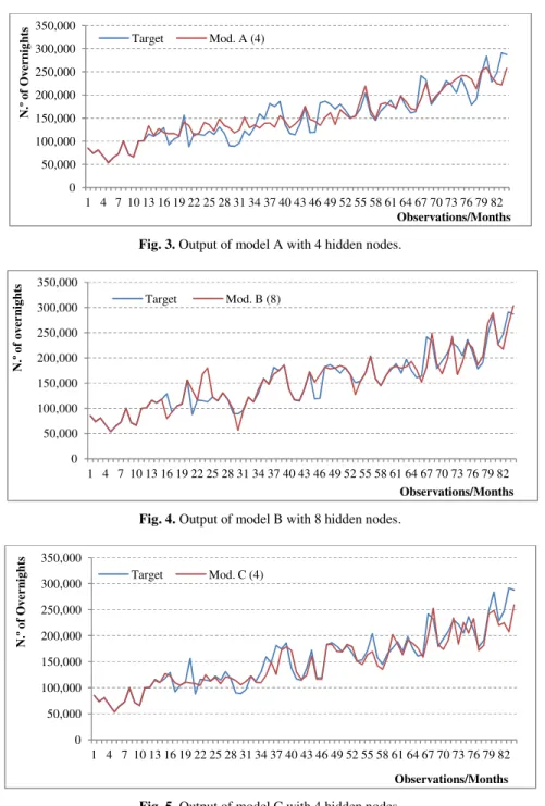
Fig. 3. Output of model A with 4 hidden nodes.
Fig. 4. Output of model B with 8 hidden nodes.
Fig. 5. Output of model C with 4 hidden nodes. 0
50,000 100,000 150,000 200,000 250,000 300,000 350,000
1 4 7 10 13 16 19 22 25 28 31 34 37 40 43 46 49 52 55 58 61 64 67 70 73 76 79 82
N
.º
o
f
Ov
er
n
ig
h
ts
Observations/Months Target Mod. A (4)
0 50,000 100,000 150,000 200,000 250,000 300,000 350,000
1 4 7 10 13 16 19 22 25 28 31 34 37 40 43 46 49 52 55 58 61 64 67 70 73 76 79 82
N
.º
o
f
o
v
er
n
ig
h
ts
Observations/Months Target Mod. B (8)
0 50,000 100,000 150,000 200,000 250,000 300,000 350,000
1 4 7 10 13 16 19 22 25 28 31 34 37 40 43 46 49 52 55 58 61 64 67 70 73 76 79 82
N
.º
o
f
Ov
er
n
ig
h
ts
Fig. 6. Output of model E with 8 hidden nodes.
Fig. 7 presents the results of the same models but only in the 12 months of the test set. It can be seen that the models captured the 3 peaks along the year. Model B are the one with values more close to the target ones.
Fig. 7. Output of test set with models A, B, C and E. 0
50,000 100,000 150,000 200,000 250,000 300,000 350,000
1 4 7 10 13 16 19 22 25 28 31 34 37 40 43 46 49 52 55 58 61 64 67 70 73 76 79 82
N
.º
o
f
Ov
er
n
ig
h
ts
Observations/Months Target Mod. E (8)
0 50,000 100,000 150,000 200,000 250,000 300,000 350,000
1 2 3 4 5 6 7 8 9 10 11 12
N
.º
o
f
Ov
er
n
ig
h
ts
5
Conclusion
The tourism time series used in this work contrary to usual tourism time series is non seasonal. This makes more challenging the task to predict future values. ANN models are adequate to solve no linear problems and were used to make predictions of this time series for twelve months of next year. Five different architectures/inputs were experimented. Model A with the 12 previous months in its input, Model B with two additional inputs for time index, Model C with only one input for the year of the time index, Model D using only 5 previous months and time index and model E with same inputs as model B but in logarithmic domain. Different number of nodes in hid-den layer was experimented.
Model B with 8 nodes in hidden layer was selected as the best model achieving an MRE of 7.3% and a correlation coefficient of 0.85 in test set.
Comparing the results of this model for this non seasonal time series with similar models for a seasonal time series, Model B achieved a similar MRE but worst correla-tion coefficient denoting the difficulty of fit the curve of this time series.
Although the apparently random values of this time series the ANN model achieved a prediction with an error that can be considered at a good level according to (Lewis, 1982).
Model C is similar as Model B but was only one variable to model the year instead of two variables to model month and year. The results showed clearly worst results for this model C. Therefore to model the time index it is actually necessary this two variables.
The input of model D has only the previous 5 months instead of 12. The results for this model were very bad denoting the real need to use the previous 12 months in the input of the model.
Model E is the same as model B, but the time series were converted to the loga-rithm domain. The results showed no improvement with model E. Therefore there is no advantage to use the log domain.
References
Algieri, B. (2006). An econometric estimation of the demand for tourism: the case of Russia.
Tourism Economics, 12, 5-20.
Cho, V. (2003). A comparison of three different approaches to tourist arrival forecasting.
Tourism Management, 24, 323-330.
Dritsakis, N. (2004). Cointegration analysis of German and British tourism demand for Greece. Tourism Management, 25, 111-119.
Fernandes, P., & Teixeira, J. (2009). New Approach of the ANN Methodology for
Fernandes, P., Teixeira, J., Ferreira, J., & Azevedo, S. (2008). Modelling Tourism Demand: A Comparative Study between Artificial Neural Networks and the Box-Jenkins Methodol-ogy. Romanian Journal of Economic Forecasting, 5(3), 30-50.
Fernandes, P., Teixeira, J., Ferreira, J., & Azevedo, S. (2013). Training Neural Networks by Resilient Backpropagation Algorithm for Tourism Forecasting. In J. Casillas, F. Martínez-López, R. Vicari, F. De la Prieta (Editors), Management Intelligent Systems, Advances in
In-telligent Systems and Computing, 220, 41-49.
Goh, C., & Law, R. (2002). Modelling and forecasting tourism demand for arrivals with sto-chastic nonstationarity seasonality and intervention. Tourism Management, 23, 499-510.
Han, Z., Dubarry, R., & Sinclair, M. (2006). Modelling US tourism demand for European destinations. Tourism Management, 27, 1-10.
INECV (2013). Anuários Estatísticos. Assessed on March 2013.
Kon, S., & Turner, W. (2005). Neural network forecasting of tourism demand. Tourism
Economics, 11, 301-328.
Kulendran, N., & Shan, J. (2002). Forecasting China's monthly inbound travel demand.
Journal of Travel and Tourism marketing, 13 (1/2), 5-19.
Lewis, C. (1982). Industrial and Business Forecasting Method. Butterworth Scientific. Lon-don.
Li, G., Song, H., & Witt, S. (2006). Time varying parameter and fixed parameter linear AIDS: an application to tourism demand forecasting. International Journal of Forecasting, 22, 57-71.
Marquardt, D. (1963). An Algorithm for Least-Squares Estimation of Nonlinear Parameters.
SIAM Journal on Applied Mathematics, 11(2), 431-441.
Palmer, A., Montaño, J., & Sesé, A. (2006). Designing an artificial neural network for fore-casting tourism time series. Tourism Management, 27, 781-790.
PEDTCV (2010). Plano Estratégico para o Desenvolvimento do Turismo em Cabo Verde. Assessed on March 2013.
Riedmiller, M., & Braun, H. (1993). A direct adaptive method for faster back-propagation
learning: The RPROP algorithm. Proceedings of the IEEE International Conference on
Neu-ral Networks.
Song, H., & Li, G. (2008). Tourism demand modelling and forecasting - a review of recent research. Tourism Management, 29, 203-220.
Song, H., & Witt, S. (2006). Forecasting international tourist flows to Macau. Tourism
Management, 27, 214-224.
Song, H., & Wong, K. (2003). Tourism Demand Modeling: A Time-Varying Parameter Ap-proach. Journal of Travel Research, 42, 57-64.