Rommel Noce1, José Luiz Pereira de Rezende2, Agostinho Lopes de Souza3, Lourival Marin Mendes4, Márcio Lopes da Silva3, Rosa Maria Miranda Armond Carvalho5, Juliana Mendes de Oliveira6, Juliana Lorensi do Canto7 (received: September 4, 2008; accepted: April 30, 2010)
ABSTRACT: This study estimated the sawn wood demand price and income elasticity.Specifically it was estimated the price elasticity of sawn wood, the cross price elasticity of wood panels and the income elasticity of Brazilian GDP. A log-log model with correction through outline of the mobile average (MA(1)) was used, adjusted for the period of 1971 to 2006, which showed to be stable, with satisfactory significance levels. It was observed that sawn wood demand is inelastic in relation to price and elastic in relation to income.
Key words: Forest economy, sawn wood demand, income maximization.
ELASTICIDADE PREÇO E ELASTICIDADE RENDA DA MADEIRA SERRADA BRASILEIRA
RESUMO: Conduziu-se este estudo, com o objetivo de estimar as elasticidades preço e renda da demanda por madeira. Especificamente estimou-se a elasticidade preço do m3 de madeira serrada, a elasticidade preço cruzada do m3 de painéis de madeira e a elasticidade renda do PIB da nação. Fez-se uso de um modelo log-log com correção por meio de esquema de media móvel (MA(1)), ajustado para o período de 1971 a 2006 que se mostrou estável e com níveis de significância satisfatórios. Observou-se que a demanda de madeira serrada é inelástica em relação a preço e elástica em relação à renda.
Palavras-chave: Economia florestal, demanda de madeira serrada, maximização da renda.
1Administrator, DS in Forest Science – Instituto de Biodiversidade e Florestas/IBEF – Universidade Federal do Oeste do Pará/UFOPA –
68035-110 – Santarém, PA – rommelnoce@yahoo.com.br
2Forest Engineer, PhD in Forest Economy – Departamento de Ciências Florestais/DCF – Universidade Federal de Lavras/UFLA – Cx.
P. 3037 – 37200-000 – Lavras, MG – jlprezen@dcf.ufla.br
3Forest Engineer, DS in Forest Science – Departamento de Engenharia Florestal/DEF – Universidade Federal de Viçosa/UFV – 36570–000 –
Viçosa, MG – alsouza@ufv.br, marlosil@ufv.br
4Forest Engineer, DS in Forest Science – Departamento de Ciências Florestais/DCF – Universidade Federal de Lavras/UFLA –
Cx. P. 3037 – 37200-000 – Lavras, MG – lourival@dcf.ufla.br
5Administrator, DS in Forest Science – Evata Educação Avançada – 36570-000 – Viçosa, MG – rosamaria@homenet.com.br
6Architect, DS in Forest Science – Instituto de Biodiversidade e Florestas/IBEF – Universidade Federal do Oeste do Pará/UFOPA –
68035-110 – Santarém, PA – julianameoli@yahoo.com.br
7Forest Engineer, DS Candidate in Forest Science – Departamento de Engenharia Florestal/DEF – Universidade Federal de Viçosa/UFV –
CEP 36570–000 – Viçosa, MG – jlcanto@terra.com.br
1 INTRODUCTION
The acquisition and merger process of the organizations is intensified by Globalization, because of the largest capital mobility and information due to the market integration which accelerated the technological development and it improved the efficiency of the productive chains, turning the competition more accentuated in quality and cost, in internal and external markets. This scenery includes the productive chains of forest based products (GARCIA, 2002).
Due to the internationalization of the economy, the consumers become more concerned with environmental issues and sustainability, placing in prominence the forest
sustained management and the origin of raw materials (CHIPANSKI, 2006).
Brazil was shown competitive in the international scenery considering products as sawn wood, plywood and furniture in spite of the high inequality indexes and of monopoly verified at the markets of these products (COELHO & BERGER, 2004; NOCE et al., 2003, 2007a,b).
260 NOCE, R. et al.
The conception of the market economy presupposes intimate relationship between price and demand. Therefore, this study aimed at estimating the demand elasticity of sawn wood. Specifically, it aimed to estimate the price elasticity of sawn wood, cross price elasticity of wood panels and income elasticity of Brazilian GDP.
2 MATERIAL AND METHODS 2.1 Proposed model
Initially it was estimated the following model:
t 3 3 2 2 1 1 0
t ß ß lnX ß lnX ß lnX u
Y
ln = + + + +
being:
Yt: sawn wood demand in m3;
X1: price in dollars for m3 of sawn wood; X2: price in dollars for m3 of wood panels;
X3: Gross Domestic Product (GDP) in thousands of dollars;
b0: intercept;
b1, b2, b3: angular coefficients;
ut: error term.
The use of a Log-Log model allows scale problems to be overcome among the variables as well as the direct obtaining of the elasticities that determine the percent variation of the demand in relation to 1% variation in prices and in GDP (GUJARATI, 2006).
The apparent consumption of Brazilian sawn wood in the period 1971-2006 was used as proxy for representing the demand of sawn wood. It was obtained by the sum of the production values and import, minus exports. The data related to the production, export and import, as well as the ones of price is available in the Food and Agriculture Organization of the United Nations - FAO (2007) website. The relative data to the Brazilian Gross Domestic Product in the referring period is available in the website of the Institute of Applied Economical Researches - IPEA (2007). Due to the autocorrelation of the error terms of the first estimated regression model, a term of movable average (MA) was inserted, envisaging the representation of the average of the recent past observations. Thus, the proposed model was:
t 3
3 2 2 1 1 0
t ß ß lnX ß lnX ß lnX MA(1)u
Y
ln = + + + +
where:
b1: price elasticity;
b2: cross price elasticity;
b3: income elasticity;
MA(1): movable averages.
The term of movable average (MA) was included in the regression model, considering that the flotation in the past values represent aleatory flotation around a “soft” curve. The larger the number of observations included in the average movable, the higher the smoothness effect in the forecast (WHEELWRIGHT & MAKRIDAKIS, 1989).
The movable averages also represent the error of aleatory events that cannot be explained by the model, i.e., the foreseen value for the observation depends on the error values observed in each past period. Besides, it can be used to soften seasonal effects (MADDALA, 2003).
The correction through the movable average to temporal series was used to estimate the ARIMA model, which made possible to distinguish the price behavior related to the wood origin, if from native or from fast growth forest (COELHO JÚNIOR et al., 2006).
2.2 Statistical analysis
The stationary stochastic process, or estacionarity of the temporal series, was tested through the test of unitary root of Dickey-Fuller. The increased Dickey-Fuller
procedure tests the null hypothesis of unitary root or non stationary temporal series (ä = 0) for the three possibilities: (a) aleatory walk without displacement ( Yt = Yt-1 + Yt-1 + ut), (b) aleatory walk with displacement ( Yt = 1 + Yt-1 +
Yt-1 + ut) and (c) aleatory walk with displacement surrounding a stochastic tendency ( Yt = 1 + 2t + Yt-1 + Yt-1 + ut). Under the null hypothesis, the value of t of
Student estimated by the coefficient Yt-1 followed the statistics (tau) and the probability of maximum error allowed was of 5%. The inclusion of lag values of the dependent variable ÄYt allowed the possibility of ut present autocorrelation (GUJARATI, 2006).
Due to the situation of estacionarity of order 1, the number of co-integration vectors was tested shared by the series through the Johansen test. It was assumed that the existence of a co-integration vector indicates that there is balance or long run relationship among the variables (JOHANSEN, 1995).
The method to estimate the regression models used was the Minimum Ordinary Square (MQO) and the result of the estimated regression was evaluated by the following criteria:
a) Determination Coefficient (R2)
The determination Coefficient (R2) is considered as
261 Brazilian sawn wood price and income elasticity
the proportion or percentage of the total variation of Y
explained by the regression model (GUJARATI, 2006). R2
was calculated by the equation:
STQ SQR 1 STQ SQE R2 being:
SQE: sum of the explained square of the regression;
SQR: sum of the square of the residue of the regression;
STQ: sum of the total square of the regression.
b) Test of general significance or F test
The general significance test (F test) was accomplished to test the null hypothesis that all the estimated coefficients are the same and equal to zero (â2 =
â3=... = âi = 0) (HOFFMANN & VIEIRA, 1998). The
calculated value of F was obtained by the equation:
k n / SQR 1 k / SQE F being:
SQE: sum of the explained square of the regression;
SQR: sum of the residue square of the regression;
k = number of estimated variables in the regression;
n = number of observations.
The statistics of the test follows the distribution F, with (k–1) degrees of freedom for the numerator and (n–k) degrees of the denominator and maximum error probability allowed of 5%. If the value of calculated F overcomes the value of critical or controlled F, the null hypothesis is rejected.
c) Test of individual significance of the coefficients or t test
Through the test t the statistical significance of the regression coefficients was verified, considering the null hypothesis that each estimated coefficient is individually equal to zero (âi = 0) (GUJARATI, 2006). The calculated value of t was obtained by the equation:
) ( ep 0 t i i being:
i = estimated coefficient;
ep = standard error of the estimated coefficient.
The statistics of the test follows the distribution t, with (n–2) degrees of freedom with maximum error
probability allowed of 5%. If the value of calculated t
overcomes the value of critical or tabled t, the null hypothesis is rejected.
d) Test of residues normality
The normality of the residues was verified through the graphic of distribution of the residues and of the
Jarque-Bera test, that considers the united hypothesis that the asymmetry (S) and the kurtosis (K) are same to zero and three, respectively (MADDALA, 2003). In that way, the test considers the null hypothesis that the residues are usually distributed. The value of Jarque-Bera was calculated by the equation:
24 3 K 6 S n JB 2 2 being:
n: size of the sample;
S: asymmetry coefficient;
K: kurtosis coefficient.
The asymmetry coefficients (S) and kurtosis (K) are given by:
n i i u u S 1 3 ˆ n i i u u K 1 4 ˆ
e
being: iu
error;u
average error;ˆ
estimated standard deviation.The statistics of the test follows the distribution of 2
(qui-square), with 2 degrees of freedom and maximum error probability allowed of 5%. If the calculated value goes superior to the critical value or tabled, the null hypothesis is rejected.
e) Autocorrelation Test
The verification of the autocorrelation presence of the error terms was accomplished through the correlogram observation and through the Breusch-Godfrey’s test (LM test) (GUJARATI, 2006).
In Breusch-Godfrey’s test the residues (ût) of the regression are obtained and estimated as dependent variable in an auxiliary regression against the independent variable Xt and its own dephased values:
t p t p t t t
t X u u u
û 1 2 ˆ1ˆ 1 ˆ2ˆ 2 ˆ ˆ
The determination coefficient (R2) of the estimated
262 NOCE, R. et al.
being:
n: number of observations;
p: number of diphase of the error term (ût).
If (n-p)R2 is superior to the critical or tabled value
at the level of maximum significance of 5%, the null hypothesis of autocorrelation absence, or that at least one
ñ is different from zero, it is rejected.
3 RESULTS AND DISCUSSION
It was observed through the test of Dickey-Fuller that the temporary series used in the study were not stationary in level, being just stationary in first difference. The use of temporary series in first difference suggests the validity of the results only for the short run temporal horizon, in case it is not verified that the variables are co-integrated. It was rejected that the series presents number of vectors of co-integration inferior or superior to two for the test of Johansen, as well as it was identified that the dependent variable regression residue by the explanatory variables is stationary (I(0)), procedure used by Mattos (2005). In that way the model was adjusted in first difference esteeming the elasticities of short run and in level to indicate the elasticities in the long run horizon, presupposing that the temporary series tend to the balance in the long run once they show co-integrated.
3.1 Short run results
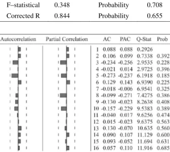
The hypothesis of absence of serial autocorrelation is not rejected by Breusch-Godfrey’s test (Table 1). It stands out that the graphic analysis of the correlogram converges for the same result of non rejection of the hypothesis of autocorrelation absence (Figure 1).
The hypothesis of normality of the residues is not rejected through the test of Jarque-Bera (Figure 2).
It was admitted that the variables are stationary in the first difference, without correlation absence and normal distribution of residues, which justified the discussion of the adjustment of the regression under a short run perspective (Table 2).
The proposed model was statistically significant by the test F (general significance) and the null hypothesis that the coefficients are jointly equal to zero was rejected at 1% of probability. The price coefficients of the sawn wood and GDP presented significant values in the test t of Student at 1% of probability, rejecting the null hypothesis of 1 e 3 equals to zero, while the price coefficients of wood panel and of the intercept didn’t show significance at 5% probability, not rejecting the hypothesis of they be equal to zero. The value of adjusted
R indicated that 96.2% of the sawn wood demand variation occurred in function of the alterations in the price of the
Table 1 –Breusch-Godfrey (LM) Test of Serial Autocorrelation. Tabela 1 – Teste Breusch-Godfrey (LM) de autocorrelação Serial.
F–statistical 0.348 Probability 0.708 Corrected R 0.844 Probability 0.655
Figure 1 – Correlogram for absence of serial autocorrelation hypothesis.
Figura 1 – Correlograma para a hipótese de ausência de autocorrelação serial.
Figure 2 –Jarque-Bera test of normality of the residues. Figura 2 – Teste Jarque-Bera de normalidade dos resíduos.
sawn wood and in GDP during the period from 1971 to 2006 (Table 2).
Table 2 – Adjustment of the proposed model. Tabela 2 – Ajuste do modelo proposto.
Table 3 – Breusch-Godfrey Test (LM) for long run Serial Autocorrelation.
Tabela 3 – Teste Breusch-Godfrey (LM) de Autocorrelação Serial para longo prazo.
F–statistical 0.453 Probability 0.640 Corrected R 1.086 Probability 0.580
Figure 3 – Correlogram for the hypothesis of absence of long run serial autocorrelation.
Figura 3 – Correlograma para a ausência de autocorrelação de longo prazo.
Figure 4 – Jarque-Bera Test of long run normality of the residues. Figura 4 – Teste Jarque-Bera de normalidade dos resíduos para longo prazo.
3.2 Long run results
Through Breusch-Godfrey’s test the hypothesis of absence of serial autocorrelation is not rejected (Table 3). This result is confirmed by the correlogram graphical analysis (Figure 3).
The hypothesis of normality of the residues was not rejected by Jarque-Bera test (Figure 4).
It was admitted that the variables are co-integrated, with autocorrelation absence and normal distribution of residues, justifying the discussion of the regression adjustment, in a long run perspective (Table 4).
The proposed model was statistically significant for the test F (general significance), rejecting the null hypothesis that the coefficients are jointly equal to zero at 1% of probability. As well as in the adjustment in first difference, the price coefficients of the sawn wood and of GDP presented significant values in
Student t test at 1% of probability, while the price coefficients of the wood panel and of the intercept weren’t significant. It stands out that the significance of the price coefficient of the wood panel presented improvement in of long run perspective. It was
Dependent variable Ln(Demand(-1))
Explanatory variable Coefficient Pattern error Test t Probability
Intercept -1.311 2.810 -0.466 0.644
Ln(price of sawn wood (-1)) -0.143 0.055 -2.591 0.014
Ln(price of wood panel (-1)) -0.053 0.064 -0.835 0.410
Ln(GDP of Brazil (-1)) 1.326 0.195 6.768 0.001
MA(1) 0.651 0.109 5.934 0.001
Statistics of the adjustment
R2 0.966 F-statistic 217.775
264 NOCE, R. et al.
Table 4 – Adjustment for the long run proposed model. Tabela 4 – Ajuste do modelo proposto para longo prazo.
Dependent variable Ln(Demand(-1))
Explanatory variable Coefficient Pattern error Test t Probability
C -0.889 2.817 -0.315 0.754
Ln(price of sawn wood) -0.140 0.056 -2.485 0.018
Ln(price of wood panel) -0.063 0.062 -1.018 0.316
Ln(GDP of Brazil) 1.298 0.197 6.589 0.001
MA(1) 0.662 0.105 6.260 0.001
Statistics of the adjustment
R2 0.965 F-statistic 220.005
Adjusted R2 0.961 Prob(F-statistic) 0.001
observed through the value of adjusted R that 96.1% of the variations of the demand were explained by the changes in sawn wood prices and by the GDP, in the period of 1971 to 2006 (Table 4).
As well as in the short run analysis, the demand was inelastic due to the coefficient of -0.140 for sawn wood price, i.e., for a 10% price variation of the sawn wood, the demand would change by 1.40% in a contrary way. The demand was elastic in relation to income, as can be observed in the coefficient of 1.298 for GDP, which indicates that a 10% change in the demand would change GDP by 12.98% in the same direction.
The demand price inelasticity presupposes that the revenue of the production would be maximized with increases of price of the sawn wood, once the demand has a reaction less than proportional to the variation of the prices. This is a coherent result with the low elasticity observed in the aggregation of wood manufactured products which includes sawn wood (CALDERON & ÂNGELO, 2006). Excessive increases of wood production would alter the offer, generating price reduction, which would reduce the income due to the inelasticity of the demand, result that confirms what would happen in the scenery of inelastic offer (ÂNGELO, 1998).
Increases in the GDP causes reactions more than proportional in the sawn wood demand, fact also observed for agglomerate panels and plywood by Brasil et al. (2003).
4 CONCLUSIONS
For the conditions in which this study was accomplished, it was concluded that:
- the increase of price favors the income maximization of sawn wood producers, both in short and long run. This is important for the sustainable use of the renewable resources, once it would be possible to combine reduction of the production with the increases of price and revenue;
- the more than proportional response of sawn wood demand to income, gives to sawn wood the status of superior good, being sensitive to structural variations;
- the values of short and long run elasticities were relatively close, as well as the significance and the coherence of the signs observed in the coefficient values.
5 ACKNOWLEDGEMENTS
To the Coordination of Superior Level Personnel Improvement (CAPES- Coordenação de Aperfeiçoamento de Pessoal de Nível Superior).
6 BIBLIOGRAPHICAL REFERENCES ANGELO, H. As exportações brasileiras de madeiras tropicais. 1998.Tese (Doutorado) - Universidade Federal do Paraná, Curitiba, 1998.
BRASIL, A. A.; ÂNGELO, H.; SANTOS, A. J.; BERGER, R.; SILVA, J. C. G. L. Demanda de exportação de painéis de madeira do Brasil. Revista Floresta, Curitiba, v. 2., n. 33, p. 135-146, 2003.
CHIPANSKI, E. R. Proposição para melhoria do desempenho ambiental da indústria de aglomerado no Brasil. 2006. Dissertação (Mestrado) – Universidade Federal do Paraná, Curitiba, 2006.
COELHO, M. R. F.; BERGER, R. Competitividade das exportações brasileiras de móveis no mercado internacional: uma análise segundo a visão desempenho. Revista da FAE, Curitiba, v. 7, n. 1, p. 51-65, 2004.
COELHO JUNIOR, L. M.; REZENDE, J. L. P.; SÁFADI, T.; CALEGARIO, N. Análise temporal do preço do carvão vegetal oriundo de floresta nativa e de floresta plantada. Scientia Forestalis, Piracicaba, n. 70, p. 39-48, 2006.
FOOD AND AGRICULTURE ORGANIZATION OF THE UNITED NATIONS. Disponivel em: <http://faostat.fao.org/site/ 381/default.aspx>. Acesso em: 15 dez. 2007.
GARCIA, J. D. Perspectivas estruturais da comercialização de produtos florestais. Brasília: Ministério do Meio Ambiente, 2002. 72 p.
GUJARATI, D. N. Econometria básica. 4. ed. Rio de Janeiro: Elsevier, 2006. 812 p.
HOFFMANN, R.; VIEIRA, S. Análise de regressão: uma introdução à econometria. 3. ed. São Paulo: Hucitec, 1998. 379 p.
MADDALA, G. S. Introdução a econometria. 3. ed. Rio de Janeiro: LTC, 2003. 345 p.
INSTITUTO DE PESQUISA ECONÔMICA APLICADA. Disponível em: <http://www.ipeadata.gov. br>. Acesso em: 10 dez. 2007.
JOHANSEN, S. Likelihood-based inference in cointegrated vector auto-regressive models. New York: Oxford University, 1995. 267 p.
MATTOS, L.B. Uma estimativa da demanda industrial de energia elétrica no Brasil: 1974-2002. Organizações Rurais e Agroindustriais, Lavras, v. 7, n. 2, p. 238-246, 2005.
NOCE, R.; CARVALHO, R. M. M. A.; CANTO, J. L.; SILVA, M. L.; MENDES, L. M. Medida da desigualdade do mercado internacional de compensado. Cerne, Lavras, v. 13, n. 1, p. 107-110, 2007a.
NOCE, R.; CARVALHO, R. M. M. A.; SOARES, T. S.; SILVA, M. L. O desempenho do Brasil nas exportações de madeira serrada. Revista Árvore, Viçosa, v. 27, n. 5, p. 695-700, 2003.
NOCE, R.; SILVA, M. L.; MENDES, L. M.; SOUZA, A. L.; SILVA, O. M.; OLIVEIRA, J. M.; CARVALHO, R. M. M. A. Preço relativo e competitividade no mercado internacional de compensado. Revista Cerne, Lavras, v. 13, n. 1, p. 51-56, 2007b.