Miguel Filipe Batista Duarte

(1)

Miguel Filipe Batista Duarte

Licenciado em Ciˆencias da Engenharia Electrot´ecnica e de

Computadores

Spectrum Sensing through Software

Defined Radio

Disserta¸c˜ao apresentada para obten¸c˜ao do Grau de Mestre em

Engenharia Electrot´ecnica e de Computadores, pela Universidade Nova

de Lisboa, Faculdade de Ciˆencias e Tecnologia.

Orientador : Rodolfo Oliveira, Professor Auxiliar, FCT-UNL

J´uri:

Presidente: Prof. Lu´ıs Bernardo Arguente: Prof. Lu´ıs Oliveira Vogal: Prof. Rodolfo Oliveira

(2)

(3)

i

Software Defined Radio

Copyright ➞ Miguel Filipe Batista Duarte, Faculdade de Ciˆencias e Tecnologia, Univer-sidade Nova de Lisboa

(4)

(5)

Acknowledgements

I would like to first and foremost thank my mentor and teacher, Rodolfo Oliveira, whose availability and helpful criticism helped me learn everything needed to complete this dissertation. I would like to thank João Porém, who has kept me company throughout all these years. Also, a big thank you to all my colleagues at FCT including but not limited to Pedro Cartaxo, Fábio Passos, Telmo Ferraria and Sérgio Pinto. To my parents, Isabel and José Duarte, who allowed me to choose this path for my life, I extend the biggest gratitude possible. I hope to be able to compensate this great sacrifice. To my brother Tiago, my second father, I can only thank for helping me in whatever I needed, whenever I needed. To my uncle Mário, I wish peace and I thank for being inspiration and an example. And last but not least, a big thank you to my loving girlfriend, Rita, who helped, distracted and overall made me a better person to this day.

(6)

(7)

Sum´

ario

Está em curso uma mudan¸ca no paradigma de controlo de transmissões de rádio. Tare-fas que já foram exclusivas de certas classes de hardware são cada vez mais realizadas por sistemas de software. Uma mudan¸ca completa para o dom´ınio do software é previs´ıvel, criando um verdadeiro conceito de Software Defined Radio. Ao mesmo tempo que esta mudan¸ca ocorre, o espectro radioeléctrico encontra-se saturado e quase completamente licenciado. No entanto, o espectro raramente é utilizado na sua totalidade ao longo do tempo, permitindo o seu uso oportun´ıstico enquanto os utilizadores licenciados não o uti-lizam. Esta é uma parte da no¸cão de Rádio Cognitivo, um tipo de rádio que permitirá acesso oportun´ıstico ao espectro. Estes dois novos paradigmas podem ser combinados para produzir um rádio flex´ıvel e fiável, ultrapassando dessa forma alguns problemas relaciona-dos com a escassez de espectro dispon´ıvel. Esta disserta¸cão come¸ca uma explora¸cão nesta ´

area combinando estes dois paradigmas através do uso de um Detetor de Energia imple-mentado através de um dispositivo do tipo Universal Software Radio Peripheral e da suite GNURadio. O desempenho do sistema é avaliado calculando as Probabilidades de Dete¸cão e Falso Alarme em cenários reais e comparando-os com os valores teóricos calculados. Um método para definir limites de decisão para sinais de banda estreita é também testado com base em trabalhos de Teoria da Informa¸cão, utilizando os algoritmos Akaike Infor-mation Criteria e Minimum Description Length. Os resultados foram obtidos através de uma transmissão real utilizando dois dispositivos USRP comunicando entre si, um agindo como utilizador licenciado e outro como utilizador secundário, oportun´ıstico. Finalmente, real¸ca-se o trabalho tecnológico desenvolvido na disserta¸cão, o qual permite testar de uma forma rápida outros parâmetros através dos scripts desenvolvidos, apresentando-se como uma ferramenta de trabalho para futuros trabalhos de investiga¸cão.

Palavras Chave: Sistemas de Rádio Cognitivo, Deteçcão baseada em Energia, Rádio Definido por Software.

(8)

(9)

Abstract

A change in paradigm when it comes to controlling radio transmissions is in course. Tasks usually executed in an exclusive class of hardware systems are increasingly controlled by software systems. A deep change to the software domain is foreseeable, creating a true Software Defined Radio. At the same time this change occurs, the radioelectric spectrum is almost completely licensed. However, the spectrum is rarely used to its full extent over time, enabling its opportunistic use while the licensed devices do not communicate. This is a part of the notion of Cognitive Radio, a new kind of radio capable of using the spectrum in an opportunistic way. These two new paradigms in radio access can be combined to produce a flexible and reliable radio, overcoming the issues with radioelectric spectrum scarcity. This dissertation starts an exploration in this area by combining these two paradigms through the use of an Energy Detector implemented in a Universal Software Radio Peripheral device and using the GNURadio suite. The performance of such a system is tested by calculating the Probabilities of Detection and False Alarm in real scenarios and comparing them to the expected theoretical values. A method for defining thresholds for narrowband signals is also tested based on works in Information Theory concepts, i.e., the Akaike Information Criteria and the Minimum Description Length. The results are tested for a real transmission using two USRP platforms communicating with each other, one acting as the licensed user and the other acting as the secondary, opportunistic user. Finally, we highlight the technological work developed in this dissertation, which may support future research works through the use of the developed scripts, allowing a faster method to test algorithms with different parameterization.

Keywords: Cognitive Radio Systems, Spectrum Sensing, Software-Defined Ra-dio.

(10)

(11)

Acronyms

ADC Analog to Digital Converter

AIC Akaike Information Criteria

ASIC Application-Specific Integrated Circuit

CORBA Common Object Request Broker Architecture

CR Cognitive Radio

DAC Digital to Analog Converter

DDC Digital Down-Converter

DUC Digital Up-Converter

DSP Digital Signal Processor

FPGA Field-Programmable Gate Array

GPP Global-Purpose Processor

GSM Global System for Mobile Communications

IF Intermediate Frequency

LTE Long-Term Evolution

MDL Minimum Description Length

MISD Multiple Instruction Single Data

MIMD Multiple Instruction Multiple Data

OSSIE Open-Source Software Communications Architecture Implementation-Embedded

(12)

x ACRONYMS

PC Personal Computer

POSIX Portable Operation system Interface

RF Radio Frequency

SCA Software Communications Architecture

SDR Software Defined Radio

SISD Single Instruction Single Data

SIMD Single Instruction Multiple Data

SNR Signal to Noise Ratio

UHD Universal Software Radio Peripheral Hardware Driver

UMTS Universal Mobile Telecommunications System

USRP Universal Software Radio Peripheral

(13)

List of Figures

2.1 SDR Basic Schema . . . 6

2.2 SDR Basic Schema . . . 7

2.3 Digital Down Converter . . . 8

2.4 Digital Up Converter . . . 8

2.5 USRP Connectivity . . . 10

2.6 USRP Base Structure . . . 10

2.7 SCA Architecture . . . 14

2.8 SCA Waveform Example . . . 14

2.9 GNURadio Architecture . . . 17

3.1 Cognitive Radio Schematic . . . 21

3.2 Cognitive Radio Sensed Spectrum . . . 22

3.3 Frame of the Secondary User . . . 23

3.4 Periodogram for a Sine Wave with Gaussian Noise . . . 26

3.5 AIC and MDL values for a Sine wave with Gaussian Noise . . . 27

3.6 Sorted periodogram of a Sine Wave with Gaussian Noise . . . 27

4.1 Secondary User GNURadio block diagram . . . 31

4.2 Primary User GNURadio block diagram . . . 31

4.3 Secondary User GNURadio Threshold block diagram . . . 31

4.4 Histogram of First USRP Experiment . . . 32

4.5 Probability of Detection and Probability of False Alarm for the first USRP Experiment . . . 33

4.6 PM iss for a range of SNR . . . 34

4.7 PM iss detail for a range of SNR . . . 34

4.8 PF A for a range of SNR . . . 35

4.9 Periodogram for a Gaussian Noise transmission . . . 36

4.10 AIC and MDL values for a Gaussian Noise transmission . . . 37

4.11 Sorted periodogram for a Gaussian Noise transmission . . . 37

4.12 Periodogram for a Sine wave transmission . . . 38

4.13 AIC and MDL values for a Sine wave transmission . . . 39

4.14 Sorted periodogram for a Sine wave transmission . . . 39

(16)

xiv LIST OF FIGURES

(17)

List of Tables

3.1 MDL and AIC Noise Estimation Values . . . 27

4.1 USRP Parameters for Energy Detection Experiment . . . 32

(18)

(19)

Chapter 1 Introduction

1.1 Introduction

Over the last 40 years, technology has validated Moore’s law [Moo06]. The number of components on a chip has consistently doubled every 18 months. This breakthrough in technology allows a processor to have capacities thought impossible just a few years ago, which opens the possibility to assign functions to processors that were only assigned to application specific hardware up until now [SRLM12]. This dissertation explores the use of processors and more specifically, software architectures to solve traditional problems in the radio domain. This technology, called Software Defined Radio, is the focus of this dissertation, which is adopted to assess spectrum sensing techniques.

1.2 Motivation

The Software Defined Radio, introduced by Mitola [Mit95], opened up a whole new world of possibilities regarding the use of radio equipments. In a world where the main agents were specifically built on circuits, the SDR contested this dogma. The main idea is to delegate some of the hardware specific tasks to software, namely baseband frequency operations, such as the generation and detection of signals [Wir].

SDR’s main objective is to add flexibility to a radio communication device, providing it with the necessary autonomy to modify radio transmission parameters through the simple loading of a script.

(20)

2 CHAPTER 1. INTRODUCTION

This flexibility allows a device to better adapt to different kinds of communication. This is something of the utmost importance in military radios [Ulv10] for example, where the need to change communication patterns in case the transmission integrity or privacy is compromised by the ”enemy” is a reality.

Another advantage is the SDR’s time-to-market. At the manufacturer level, when a new wireless architecture (e.g. transmitter/receiver scheme) is required, less hardware and more software development is needed to implement new features, greatly decreasing the development time. Thus, time-to-market is greatly reduced while innovation grows [PRL+_12].

The Cognitive Radio is an evolution in the paradigm of spectrum usage. It relies on the fact that a Secondary, unlicensed user can identify if the spectrum is being accessed by a Primary, licensed user. The reliability of this method must be high, since the interference caused to the licensed users must be avoided. Knowing if the spectrum is being used or not allows the Secondary User to control its transmission power and frequency occupation, therefore using a licensed frequency and increasing spectrum usability.

The main objective of this work is to evaluate the actual performance of SDR tech-nology to perform Spectrum Sensing.

1.3 Objectives and Contributions

The first objective of this dissertation is validating through practical SDR experiments the Probabilities of Detection and False Alarm that characterize the ability of an Energy Detector to successfully identify the presence/absence of a Primary User in the sensed spectrum. For this end, a script that tests these probabilities was designed using the GNURadio software suite. This test allows the characterization of the Energy Detector within a range of different SNR values.

(21)

1.4. STRUCTURE OF THE DISSERTATION ₃

eigenvalues, avoiding the need of a square matrix to compute eigenvalues and increasing the flexibility of the scheme, allowing for an arbitrary number of FFT samples to be collected.

The practical validation of the theoretical values ofPD andPF A for a predefined

sens-ing time have already contributed to the article presented in DOCeis 2014[MD14], titled

Practical Assessment of Energy-based Sensing through Software Defined Radio Devices.

1.4 Structure of the dissertation

(22)

(23)

Chapter 2 Software Defined Radio

2.1 Introduction

Reconfigurability is the main characteristic at the core of the SDR concept. Over the years, the evolution of telecommunications has brought technologies such as GSM (Global System for Mobile Communication), UMTS (Universal Mobile Telecommunications Sys-tem) or more recently LTE (Long Term Evolution) to life.

Although the communication schemes supporting each technology are different, their objective remains the same: transmit and receive voice and data. SDR proposes to unite some of these technologies in a single device, switching between them as needed. This proposition is achieved by adding flexibility to the radio equipment. Reconfigurability, however, is practically non-existent nowadays as radio tasks are handled by application-specific hardware devices. The SDR concept, however, allows for radios to be configurable, even programmable in software to a large extent, with the help of software-controlled technologies. The need for this concept stems from the different transmission quality and QoS needs nowadays when performing a vertical handover from one radio standard to another (e.g. Switching from GSM to LTE on a phone).

A system that satisfies these flexibility needs via software controlled components is an SDR.

(24)

6 CHAPTER 2. SOFTWARE DEFINED RADIO

Front-End RF

ADC/DCA

Processor

Figure 2.1: The basic schema of a SDR architecture

2.2 Hardware Architecture of an SDR

A basic Schema of SDR is presented in Figure 2.1. In the figure the Processor is represented as a single block. However, it can comprise several processors working in parallel. Theoretically there could be only one processor computing all the code. In practice the work of processing a signal is too demanding most of the time for a single processor, so the processor block can include an array of components that are built to manage waveforms and the processing needs associated with them.

Some of the hardware solutions featuring mostly multi-core processors are presented in [PRL+

(25)

2.2. HARDWARE ARCHITECTURE OF AN SDR ₇

RF TX

Interface InterfaceRF RX

1..n

....

. ... 1..n

Processor

DUC DDC ADC

DAC

Figure 2.2: Basic Schematic of an SDR Architecture

2.2.1 General Hardware Architecture

The hardware architecture of a SDR system may vary, depending on its flexibility. There might be a need to change only one or all of the operational aspects of the ra-dio. Thus, the hardware technology may change as well. A general design of an SDR is presented in Figure 2.2.

As can be seen in Figure 2.2, there may be more than one antenna attached to the RF front-end. This is due to the fact that by switching transmission protocols and supporting MIMO transmission, SDR systems can work in different frequencies covered by different antennas. Thus, SDR systems must have capabilities of switching antennas when they need to switch the operational frequency.

There are three distinct blocks for Downlink and Uplink.

Downlink Structure

The Downlink is responsible for receiving and decoding data. The first block in this chain is the RF front-end. This block is ideally reconfigurable for a wide range of frequencies and holds the interface between the Intermediate Frequency (IF) and Radio Frequency (RF) parts of the system. It generally consists of a Band-Pass Filter to eliminate undesired frequencies, a Low-Noise Amplifier to amplify the desired signal and a Mixer, responsible for converting the signal from RF to IF by mixing it with the Local Oscillator signal.

(26)

that for most of the signals, this conversion is only technologically possible because the central frequency of the original RF signal was decreased to the feasible (IF) levels in the RF front-end.

After the ADC the digital signal enters the Digital Down Converter (DDC), illustrated in Figure 2.3.

IF Quadrature Sinusoid sin cos X X Low-Pass Filter Low-Pass Filter Downsampler Downsampler Iout Qout Iin Qin

Figure 2.3: Digital Down Converter generic schematic

The DDC is responsible for bringing the signal down to baseband in order to be processed by the software. It is composed by an IF Sinusoid Multiplier, a Low-Pass Filter and a Downsampler. The Multiplier brings the signal down to baseband where digital signal processing is more feasible. The Low-Pass filter eliminates undesired clones created by the multiplication. Finally, the Downsampler throttles data so that it will achieve the necessary rate to pass through the BUS connecting it to the processor.

After this conversion the signal is brought to the processor, where it will be processed by software.

Uplink Structure

The Uplink is responsible for generating and transmitting data. This data, as opposed to Downlink, is generated in the processor and transmitted through the BUS. It is then sent to the DUC (Digital Up Converter) (Figure 2.4).

IF Quadrature Sinusoid sin cos Interpolator X X Iout Qout Iin Qin Interpolator To DAC

Figure 2.4: Digital Up Converter generic schematic

(27)

2.2. HARDWARE ARCHITECTURE OF AN SDR ₉

up to IF frequencies. It consists of an Interpolator to increase the sample rate and a Multiplier to convert the signal. At this stage no filter is needed because the signal will be filtered in the RF block.

The signal is then passed to the DAC (Digital to Analog Converter), which does the opposite of the ADC. It transforms the parameterized signal into an analog signal through interpolation, readying it for up-conversion to RF and transmission by the RF block.

The RF block then takes this IF analog signal, converts it to RF, filters it to match only the desired frequencies and transmits it. This block is responsible for power control of the transmission.

2.2.2 USRP Case Study

The Universal Software Radio Peripheral (USRP) is a front end device designed for SDR purposes. USRPs consist of a motherboard and several possible daughterboards [Ett]. The motherboard contains an FPGA for signal processing, Digital to Analog Converters, Analog to Digital Converters, an interface to access the GPP linked to it and a power control device. The daughterboards contain the RF part of the device, converting the baseband signal to the desired frequency and transmitting it over an antenna.

The USRP is controlled by the USRP Hardware Driver, UHD. The UHD contains firmware to work with the built-in FPGA and the signal converters. The USRP uses the strategy described in Subsection 2.2.3, delegating all redundant and high bandwith operations to the FPGA [RYZ11] to reduce sample rate sent to the peripheral processing unit. This unit could be a GPP, as mentioned before, and is connected to the USRP via an interface (e.g., USB or Gigabit Ethernet). The UHD ensures that the data is sent through the USB and returned after processed. Figure 2.5 shows the general architecture of the system.

There are, of course, several limitations in terms of the technology adopted in USRP devices. One of them is the main connection method to the processor, which adopts the USB 2.0 standard. It has been calculated that its data rate is of approximately 32MS/s (MegaSamples/second) and its bandwidth can not exceed 12MHz [RYZ11].

(28)

PC

FPGA

USRP

UHD

Instructions

Processor

RF Front-end (Daughterboard)

UHD

Figure 2.5: URSP connectivity to a PC and processing options

implemented using the USRP. This is one of its greatest shortcomings.

USRP Structure

The structure of a USRP device is kept as simple as possible. Nevertheless, some explanation might be required to explain how its components work and connect to each other.

FPGA Daug

ht er boa rd In te rfa ce Da ug ht er boa rd UHD Data Streaming PC Interface DAC ADC DDC + Decimator Interpolator +DUC

Figure 2.6: USRP basic structure. Changes apply between different models.

(29)

2.2. HARDWARE ARCHITECTURE OF AN SDR ₁₁

is up to the user to change these settings according to the objectives. The figure also shows the ADC and DAC components, responsible for the Analog/Digital conversions. The performance of all these components varies from USRP model to model.

The UHD Data Stream controls the information from/to the PC and the PC Interface exchanges data between the devices through it. This interface can be a USB for some USRP models or a Gigabit Ethernet connection for others.

The daughterboards implement the RF front-end of the USRP. Several types of daugh-terboards are available, each one with their specific frequency range. The portfolio of dif-ferent daughterboards allows the use of the USRP in most of the commonly used frequency ranges, all in the same device (same motherboard with different daughterboards).

2.2.3 Processing Options

The paradigm change associated with SDR brings challenges not faced before. One of them is finding the optimal hardware design for signal processing. There are many different options to handle the signal processing, and the main trade-offs involved in their choice are the level of performance and flexibility. In this section we will explore several systems already proposed for signal processing.

Application Specific Integrated Circuits

Application Specific Integrated Circuits (ASICs) are the de facto devices adopted in Digital Signal Processing. ASICs are circuits designed and built for one purpose specifically and can not be reprogrammed, meaning they are not a good choice for more flexible solutions. ASICS are, therefore, not compliant with the notion of SDR. However, some authors [SIW06] suggest that similar operations between waveforms should be studied and applied in ASICs whenever possible, in detriment of waveform global portability.

Reconfigurable Processing Elements

(30)

as the need of processing a different waveform. These are widely used pieces of machinery for digital systems, with the downside of consuming more energy and occupying more space than ASICs.

The processing capabilities of FPGAs are similar to ASICs’, but FPGAs are on average 3.2 times slower than ASICs [KR07]. This is much of the tradeoff between a fixed and programmable processing unit and one of the technical challenges with SDR, the processing speed.

An advantage of using FPGAs is their massive use nowadays. There are many useful toolsets already available in the market to work with SDR and FPGAs. One of these tools translates c-code into FPGA code, i.e. Very High Speed Integrated Circuits Hardware Description Language (VHDL)[LBJ06]. This implies the possibility of side-processing done by FPGAs alongside General Purpose Processors (Subsection 2.2.3). It could be especially useful for mathematical intensive computations.

Global Purpose Processor

These are everyday processors one might find in almost every piece of electronic equip-ment nowadays. The impleequip-mentation of the functions associated with waveforms is done at a much higher level than the hardware-based solutions. This implies higher latency but much higher flexibility.

The recent evolution of the GPP has migrated from increasing its clock speed to increasing the parallelism between components and increasing the number of processors in a single socket. This means a more suited type of processing for digital signals, due to the need of multiple and redundant operations when dealing with radio.

Currently there are four types of data processing associated with GPPs: Single In-struction Single Data (SISD), Multiple InIn-struction Single Data (MISD), Single InIn-struction Multiple Data (SIMD) and Multiple Instruction Multiple Data (MIMD).

(31)

de-2.3. SOFTWARE ARCHITECTURE OF AN SDR ₁₃

fined order, but only once at a time independently of how many processors are available. This opens the possibility to distribute common processes through different processors, imposing parallelism on the system when needed. An example of the application of such a feature would be sensing (verifying data being transmitted) through two different anten-nas, for two different frequency ranges. This would imply Fourier Transforms computed in parallel with two data sets, one per antenna. It would therefore benefit from the SIMD advantages.

MIMD processors distribute data and instructions through different processors as long as they are in line to be executed. This allows more flexibility in executing parallel tasks, allowing for a greater variation in parallel operations. Most of the processors available today are MIMD.

Despite its advantages, GPPs exhibit high energy consumption. These processors were not built for portable devices, at least not as small as a cell phone. Therefore, a battery would not last enough time to make GPPs a good choice to use in portable devices.

On the other hand, GPPs are most appropriate for academic and amateur applications. Most people own a computer, and that is a fact that plays strongly in GPPs’ favor. Also, a GPP can be used together with an FPGA, for example, to compensate for any shortcomings it might have.

2.3 Software Architecture of an SDR

The Software Architecture of an SDR system specifies the way the software is orga-nized to handle the data received from the antenna and the way it generates the data for transmission. It is inevitably a complex system, taking into account that all operational circumstances must be tackled. Three examples will be given in this section.

2.3.1 Software Communications Architecture

(32)

features listed in Section 1.2, namely the ability and speed to adapt to different radio parameters. The need to change the pattern of communication when it is compromised is a reality in the theater of war. Thus, JPEO created this framework which consists of a set of rules to obey when constructing a robust radio system compatible with SDR. SCA is not the only framework available, as seen later in the section, but it is a reference architecture that must be studied due to its importance in the current state of the art.

Hardware Board Board Support Package

Operating System and Network Stack

CORBA SCA Core Framework

Logical Bus (Middleware)

C1 C2 C3 C4

}

Ap plic ation s

}

O pera tion al E nvi ron m en t

Figure 2.7: SCA Architecture, with the correspondent Core Framework.[Adapted from [SCA]]

Figure 2.7 presents the general structure of the framework. Each application repre-sented in the figure(i.e. C1, C2, C3, C4) is a waveform. Waveform is the generic term for a complex radio structure. An example of a waveform is represented in Figure 2.8.

USRP CHAN_FILT _DEMFM AUDIO FILT +

DECIM. (5) AUDIO FILT +DECIM. (2)

MONO 2 STER

Figure 2.8: SCA Waveform Example, with high granularity

(33)

abstrac-2.3. SOFTWARE ARCHITECTURE OF AN SDR ₁₅

tion and independence by using common instructions in the hardware, supported by the Board Support Package.

The Operating System must be a Real Time Operating System, compatible with POSIX [Pos]. The Core Framework (CF) components have complete access to the OS, in order to call the services needed to execute the application.

The CF and the Common Object Request Broker Architecture (CORBA) standard are probably the most important parts of SCA. CORBA is used due to its flexibility, allowing the CF to distribute applications with platform independence and openness. This is achieved by using an Object Request Broker, or ORB, to manage applications and resources.

While ORBs are mainly supported by GPPs, special ORBs for working with SCA that provide a faster access to resources have been designed. These ORBs use DSPs and FPGAs in order to raise the system’s portability [Hum06]. However, since all resources rely on CORBA to be handled, there is a significant overhead associated with each appli-cation. This is due to CORBA’s characteristics such as message marshalling and location variation for resources. So, on one hand there is the mobility and flexibility earned by using CORBA. On the other, CORBA may degrade the computational time required to execute a given task. This issue can be mitigated by switching transport protocols with TCP/IP, CORBA’s default protocol, which minimizes overhead [Doh02][BCMR02]. Also, CORBA has known issues with computation and memory resources, diminishing its pop-ularity in some domains [Ulv10]. This fact raises the question: should SCA continue to exclusively use CORBA?

(34)

OSSIE

Open-Source SCA Implementation-Embedded (OSSIE) is a project started by Wire-less @ Virginia Tech, with the intent to distribute and facilitate access to the SCA frame-work. Most of the interfaces present in SCA are part of OSSIE [SCA]. However, some of them are already configured, which means that OSSIE is not as flexible as SCA is due to its complexity

OSSIE is written in C++ and uses omniORB and Xerces XML for parsing. It is developed for Linux. There is also the OSSIE Waveform Workshop, a set of tools designed to ease the work of a radio engineer.

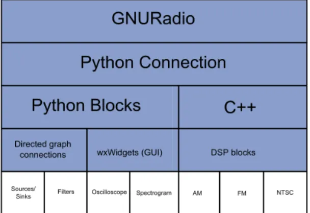
2.3.2 GNURadio

GNURadio (GR) is an open source project that consists of a software-only approach for radio applications design. It can be connected to hardware for real world use or simulated in a conditioned environment.

GNURadio implements simple modules described by C++. Digital Signal Processing (DSP) is almost all done in software, hence there is a need to separate and categorize these modules.

GNURadio provides signal generators (sources), receivers (sinks) and intermediate blocks (filters). These blocks are linked through Python, defining the final schema to be tested. Python does nothing more than connect these blocks, which has generated some discussion regarding efficiency and the need for this extra layer of Python [TT09].

The general structure of the GNURadio architecture is represented in Figure 2.9. As depicted in the figure, graphical blocks and connections are built in Python, as opposed to all other DSP blocks which are built in C++.

Since GR is an open source project any user, amateur or professional, can contribute to extend the existing libraries, even to change the way GR works from its root.

2.3.3 A Comparison of SCA (OSSIE) and GNURadio

(35)

2.4. CONCLUSIONS ₁₇

Python Connection

Python Blocks C++

Directed graph

connections wxWidgets (GUI) DSP blocks

Sources/

Sinks Filters Oscilloscope Spectrogram AM FM NTSC

GNURadio

Figure 2.9: GNURadio blocks and applications, divided by layer.

and, therefore, difficulty. Its greatest advantages come from seamless distributed process-ing thanks to CORBA [BCMR02] and its numerous layers of security [MBF05]. However, some of its drawbacks are also due to CORBA.

In a comparative study between OSSIE and GR [ALRD+

08] both systems are eval-uated according to different features that are independent of the hardware schemes that can be adopted. The main conclusion highlighted in the study is that OSSIE requires more processing power and memory usage, exhibiting 5 times more CPU load and 2 times more memory for the same waveform.

It is also important mentioning that in a GNURadio environment the latency is 25 times shorter than that present in OSSIE. This larger latency in OSSIE is mostly due to the overhead introduced by CORBA. Therefore, for low budget (low hardware capacity) and non-commercial tests on waveforms, GNURadio seems like the most appropriate setup.

2.4 Conclusions

(36)

price and functionality. Since the platform allows for a great flexibility with the change of daughterboards, the platform is guaranteed to be a good choice for experiments.

The software solutions regarding SDR are still limited but flexible and complete. With investment in the area and the contribution of the open source community, solutions like SCA and GNURadio will see an evolution in the future and will permit model designing and testing for a wide array of platforms and communication patterns. Since SCA is a more complex solution, for low budget operations and investigations GNURadio will probably be chosen as a testing platform for most academic experiments, enlarging the user base and the number of contributions to the system.

(37)

Chapter 3 Cognitive Radio

3.1 Introduction

The radioelectric spectrum is a scarce resource. With the exponential increase verified in the last years in consumer electronics, there is a dangerous spectrum shortage right now. This fact needs to be overcome. However, as noted in [MSB06], most of the spectrum is underused, but most of the bands are allocated to several licensed users. This means that there is an opportunity to use those bands while they are vacant. One of the most recent and important applications for the use of this opportunity is the dynamic use and allocation of radio spectrum. The radios that can accomplish this are called Cognitive Radios (CR).

Cognitive Radio, a term introduced in [MMJ99], proposes to analyze the radio spec-trum, estimate the state of the channels, predict what is going to happen and manage it’s spectrum, transmissions and power according to that information. Simon Haykin has defined for Cognitive Radio as follows [Hay05].:

Cognitive radio is an intelligent wireless communication system that is aware of its

surrounding environment (i.e., outside world), and uses the methodology of

understanding-by-building to learn from the environment and adapt its internal states to statistical

vari-ations in the incoming RF stimuli by making corresponding changes in certain operating

parameters (e.g., transmit-power, carrier-frequency, and modulation strategy) in real-time,

with two primary objectives in mind:

(38)

20 CHAPTER 3. COGNITIVE RADIO

❼ highly reliable communications whenever and wherever needed;

❼ efficient utilization of the radio spectrum.

Because of these characteristics, a CR needs reconfigurability. This is achieved by using SDR platforms, introduced in Chapter 2.

Cognitive Radio has been studied widely in [MMJ99] and [Mit00] and it improves the band’s utilization. In this dissertation we will focus on the first part of a cognitive radio operation: the Spectrum Sensing.

3.2 Spectrum Analysis

The basis of the cognitive radio lies on the analysis of the spectrum, also known as

Spectrum Sensing. A CR must know the level of occupancy of the radio spectrum in order to take action, and in order to do this it must sweep large ranges of frequencies. This raises the first problem: How does a radio effectively sweep such a large range of spectrum? This dissertation evaluates a response to the question by using a Software Defined Radio platform.

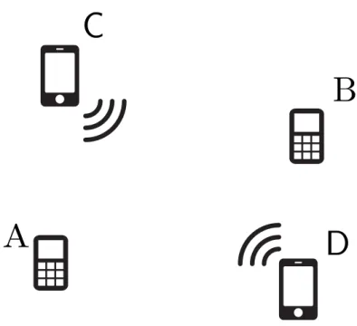
There are two classes of spectrum users, Primary Users (PUs) and Secondary Users (SUs). A PU has licensed access to the spectrum while an SU needs to use it opportunis-tically in order not to interfere with any PU. Consider the scenario illustrated in Figure 3.1. SU A wants to communicate with SU B but it first has to check if there is spectrum available for its transmission. It is a simple case of A-B transmission.

Considering that radios C and D are communicating in a part of the band sensed by the SUs, the spectrum should appear to these SUs as shown in Figure 3.2. After the sensing period and the conclusion that Channel 2 is being used, the SUs would switch to Channel 1 and transmit their data.

(39)

3.2. SPECTRUM ANALYSIS ₂₁

A

B

C

D

Figure 3.1: Secondary Users A, B and Primary Users C,D.

objective is, however, being able to utilize all the spectrum, so one technique is unlikely to work for all technologies and frequencies.

There are limits concerning Spectrum Sensing. Due to the sample rate being entirely connected to the range of frequencies analyzed (Nyquist’s theorem), the rate at which data can be gathered, transferred and processed is linked to the frequencies that a cognitive radio can analyze. For example, in a USRP device connected by USB 2.0, the theoretical limit is closely tied to the connection’s top speed at 35MB/s. The antenna configuration is another important point. For sub-optimal receiving areas, an antenna might detect a non-existent transmission. The problem is minimized when an array of antennas cooperating in sweeping the frequencies is adopted.

The spectrum sensing technique studied in this dissertation is the Energy Detection, which was theoretically characterized in [Urk67]. It relies on energy sensing and threshold comparison in order to detect the presence of a transmission.

According to [ALL10], the ability to detect a signal involves the evaluation of two hypothesis:

H0:y(t) =n(t) H1:y(t) =n(t) +s(t)

(40)

f P

Channel 1 Channel 2

Noise Floor

Figure 3.2: RF Spectrum, as sensed by A and B.

wherey(t) represents the received signal,s(t) denotes the transmitted signal andn(t) represents the noise experienced during the signal reception.

The noise vector n(t) is assumed to be additive, white and Gaussian (AWGN) with zero mean and variance σ2

n. For the purpose of this work, the signal s(t) is also assumed

to be a Gaussian random variable with varianceσ2

s.

In other words,

Y _∼

   

  

N(µn, σ2n), H0

N(µs+µn, σs2+σ

2

n), H1

(3.2)

The probabilities associated with detecting a transmission are the Probability of De-tection (PD) and Probability of False Alarm (PF A). These are defined as follows:

PD(γ) =P r[Y > γ|H1] (3.3)

PF A(γ) =P r[Y > γ|H0], (3.4)

γ is a decision threshold used to compare the received energy.

Assuming NS samples collected during the detection, PD and PF A can be rewritten

(41)

3.2. SPECTRUM ANALYSIS ₂₃

PD(γ) =Q(

γ₋NS+θ)

p

2(NS+ 2θ)

) (3.5)

PF A(γ) =Q(

λ₋NS

√

2NS

) (3.6)

whereθ=PN s

k=1(µs/(1 +σs)) 2

=PNS

k=1θ ′

and the Q function is the tail probability of the standard normal distribution:

Q(x) = √1

2π ∞

Z

x

exp(₋u 2

2 )du (3.7)

In this dissertation it is assumed that there isa priori knowledge of the signal and noise probability distributions. The purpose of this kind of testing is evaluating the performance of an SDR device, in this case a USRP, when performing these tasks.

Proposed Energy-Based Detection Model

The proposed model in this dissertation is called a periodogram. This model com-putes the Fast Fourier Transform (FFT) of the samples collected by the USRP, translating them into the frequency domain.

N1 NS NS+1 NT

TSSU TDSU

... ... ... ... ... ...

Figure 3.3: Secondary User Frame

In the proposed model the SU has a frame structure that distinguishes two differ-ent tasks: Sampling and Transmission. Sampling happens during the TSU

S period, which

depends on the number of Sensing Samples and the Sampling Rate of the SU. The trans-mission may occur during the TSU

D , if the SU detects the spectrum is not occupied. To

(42)

Xk= NF F T

X

n=0

xne−i2πk

n

N, k= 0, ...N_S−1 (3.8)

This spectrum description can allow for some criteria to be used. In this model, these values are averaged, for an average power per sample (Yn). Given that the FFT size is

equal to the number of sensing samples, NS, the average is calculated by

Yn=

1 NS

NS−1 X

k=0

|Xk|2 (3.9)

Each of theseYn values is then compared against the decision threshold,γ, to decide

if a PU is present or absent.

To validate the detection there is a previous knowledge of whether the PU is present or absent. In the validation, the practicalPD andPF A values are calculated directly from

the comparison done in the energy detected, being its output given by Bn and Cn. To

compute PD it is assumed that:

Bn=

0, Yn< γ|H1 1, Yn> γ|H1

(3.10)

To compute PF A,Cn is defined as follows:

Cn=

0, Yn< γ|H0 1, Yn> γ|H0

(3.11)

Each of the probabilities is then calculated by:

PD = _M1 P M n=0Bn PF A = _M1 P

M n=0Cn

(3.12)

where M is the number of decisions. There are some trade-offs to consider when using this approach. Parameters such as the ratio between NS and NT, the desired frequency band

(43)

3.2. SPECTRUM ANALYSIS ₂₅

Decision Threshold Estimation in Presence of a Signal

The aforementioned methods work for cases where the noise power and the presence or absence of a PU are known. However, in cases where the SU knows the PU is transmitting but has no means of knowing the noise values, the threshold can not be calculated by inspection. Some methods were already defined to calculate the value for this threshold when no prior knowledge about noise is available.

The methods studied in this dissertation are the Minimum Description Length (MDL) and the Akaike Information Criteria (AIK), derived from [WP98] and [WK85]. These algorithms also depend on the presence of a signal. Both algorithms use eigenvalues to in the decision process. However, in this case the eigenvalues are considered to be the values of a sorted periodogram, calculated by:

Pk=|Xk|2 (3.13)

It is then considered that the eigenvalue of the k-th FFT is

λi =Pk (3.14)

The AIC and MDL values are then calculated by [SMS12]:

AIC(k) = (N ₋k)Llog(α(k)) +k(2N₋k) (3.15)

and:

M DL(k) = (N₋k)Llog(α(k)) +k/2(2N₋k)log(L) (3.16)

where:

α(k) =

PN

i=k+1λi

N−k

(QN

i=k+1λi)

1 N₋k

(3.17)

(44)

approx-26 CHAPTER 3. COGNITIVE RADIO

imated by Pk.

Both algorithms evaluate the periodogram and draw conclusions in regard to its shape. The valuekis the model number and it ranges from the values 1 toN (FFT Size). For each of these values there is an MDL and AIC corresponding value. The model number with the lowest AIC and MDL value is defined as the threshold for the signal power in the averaged periodogram. Up to that k value, a primary user is considered as being active (detected). From k to N a channel is declared as idle, allowing the calculation of the average noise power.

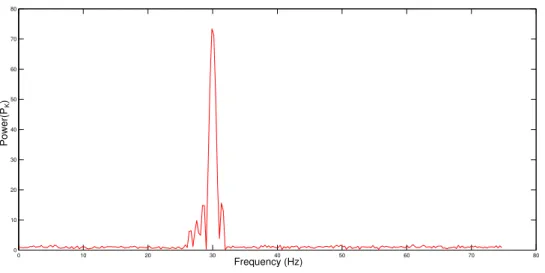
These two models were tested for a periodogram generated in MATLab. The peri-odogram represents a sine wave centered at 30 Hz and sideband AWGN Noise with its power centered at 1. This periodogram is presented in Figure 3.4.

0 10 20 30 40 50 60 70 80

Frequency (Hz)

P

o

we

r(

PK

)

Figure 3.4: Sine wave with sideband Gaussian Noise

(45)

3.2. SPECTRUM ANALYSIS ₂₇

0 50 100 150 200 250 300

1 2 3 4 5 6 7 8 9 10x 10

4 X: 18 Y: 2.029e+04 X: 18 Y: 1.584e+04 MDL AIC M D L/A IC

Model Number (k)

Noise Signal

Figure 3.5: AIC and MDL values for a Sine wave with Gaussian Noise

0 50 100 150 200 250 300

0 10 20 30 40 50 60 70 80 X: 18 Y: 2.132

Model Number (k)

P o we r( PK )

Figure 3.6: Sorted Sine wave periodogram with Gaussian Noise

With this data, the noise figure was calculated through averaging all points in Figure 3.6 from the valuekAI C whereAIC(kAI C) =min(AIC) andkM DLwhereM DL(kM DL) =

min(M DL) upwards. The results are presented in Table 3.1.

Waveform Real Noise Figure Noise Estimation (AIC)

Noise Estimation (MDL)

Sine+Noise 1.00 1.00 (kAI C=18) 1.00 (kM DL=18)

Table 3.1: MDL, AIC Noise values estimation

(46)

take into account the relationship between the power throughout the whole spectrogram and not particular waveforms, the estimation is very accurate. It correctly identifies the peak as being the signal, singles out the power values for that peak and averages the other samples in the periodogram for a perfect estimation of the noise figure.

There is a parameter that can be varied with a high effect on the output, L. In this experiment, L was set to 1000. The ideal value for this parameter would always depend on a case by case scenario, since the bandwidth and the amplitude of the sensed wave influence the output of the criteria.

3.3 Conclusions

(47)

Chapter 4 Experiments on EBS

Parametrization

4.1 Testbed Description

The proposed EBS model was tested on a setup with two USRP B100 connected to a PC with the following specifications:

❼ OS: Ubuntu 12.04 64 bit

❼ Memory: 4GB DDR3

❼ Processor: Intel Core i5-2320 @ 3.00GHz x 4

❼ Hard Drive: 320GB @ 7200rpm

The GNURadio version installed was the 3.7.1 and the USRP driver was UHD 003.005.003, the latest versions available at the time of the experiment.

The two USRPs consist of a motherboard with a Xilinx Spartan 3A 1400 FPGA, 64MS/s dual ADC, 128MS/s dual DAC and USB 2.0 connection. These motherboards used as a front-end device an SBX 400-4400 MHz Rx/Tx Daughterboard, with two RF ports: a transceiver (TX/RX) and a receiver (RX2). The daughterboard provides up to 100mW of output power and a typical noise figure of 5dB.

The USRPs were connected to each other (TX/RX to RX2) through a coaxial cable and two 30dB, 50Ohm attenuators to achieve lower SNR when transmitting.

(48)

30 CHAPTER 4. EXPERIMENTS ON EBS PARAMETRIZATION

4.2 Experiment Description

The experiment consisted of three steps, described in detail in the following Subsec-tions:

1. Determine, noise and signal data, determine thresholds

2. Collect data with regard to calculated thresholds

3. Detector characterization

The main objective is the comparison between the theoretical distribution of proba-bility and the real distribution, by calculating the practicalPD and PF A using the USRP

in real-time.

To achieve that, a python script was built in which the USRP parameters are defined. The steps were done as follows:

4.2.1 Noise and Signal Data Computation

The script allows the user to select parameters such as:

❼ Frequency (Hz) - Operational frequency of the SU and the PU (in case of PU

trans-mission);

❼ Sample Rate (Samples/s) - The sample rate at which the SU and the PU receive

and transmit data. The observed spectrum bandwidth follows Nyquist’s rule, Fs/2;

❼ Packet Size (Samples) - The number of samples of a packet (NF);

❼ Sensing Samples (Samples) - The number of sensing samples in a packet (NS);

❼ Transmitter Gain (dB) - The output gain on the PU in case of transmission;

❼ Receiver Gain (dB) - The gain of the SU;

❼ Sensing Time (s) - The required for calibration;

❼ Noise File Name (String) - The name of the file where noise data is stored;

(49)

4.2. EXPERIMENT DESCRIPTION ₃₁

USRP Y Samples

Keep N

in Y FFT N pts. | |²

Average N points

Save Average To File

Figure 4.1: Secondary User GNURadio block diagram

Noise

Source Throttle

USRP Sink

Figure 4.2: Primary User GNURadio block diagram

The script then does two data collections: one where the PU is transmitting and one where it is not. The GNURadio design blocks for the PU and the SU are illustrated in Figures 4.1 and 4.2.

The µ, σ values of a normal approximation of the values present in the averaged periodogram are then calculated through the use of the Python NumPy library.

Three files are obtained: a binary file containing the signal spectrogram averages, a binary containing the noise spectrogram averages and a file containing the parameters used in the transmission.

The decision threshold range is defined on the lower bound by the minimum value of the noise spectrogram and on the higher bound by the maximum vale of the signal spectrogram.

4.2.2 Data gathering with parametrized thresholds

This part of the script loads the .dat files associated with noise and signal and the properties.p file related with the operational parameters. In this part of the experiment, a threshold block is added to the signal processing unit. This threshold was set for aPF A

value of 5%, according to the theoreticalPF A curve. For each previously defined threshold

the block diagram in Figure 4.3 is executed and the results registered, first with the PU transmitting and then with the PU silent.

USRP Y Samples

Keep N

in Y FFT N pts. | |²

Average N

points Threshold

(50)

4.2.3 Detector Characterization

The Energy Detector was characterized by calculating its Probability of Miss-Detection, PM iss= (1−PD), after setting a threshold value (in this experiment, at PF A= 5%) and

changing the transmitter power, thus changing the SNR. The script allows the user to choose what range of SNR is desired in comparison with the original, as well as the num-ber of periodogram averages that should be collected. It then calculates the PM iss values

for each experiment and its corresponding value of SNR, increasing the SNR value for each iteration. This allows the evaluation of the Energy Detector’s performance under a wide range of SNR.

4.3 Experimental Results

The first experiment was done assuming the following set of parameters:

Frequency (GHz)

NS NT Sample

Rate SU Gain (dB) PU Gain (dB) SNR (dB) Primary AWGN Amplitude

1.3 256 5120 1,000,000 10 10 -6.5 0.0001

Table 4.1: USRP Parameters for Experiment

The histogram of the collected data and the approximated normal distribution calcu-lated with basis in this collected data for noise and signal characterization can be seen in Figure 4.4.

3 4 5 6 7 8 9 10 11 12 13

x 10−7

0 1 2 3 4 5 6 7 8

9x 10

6 Received Energy Number of Occur rences Signal Histogram Signal Normal Distribution Noise Histogram Noise Normal Distribution

(51)

4.3. EXPERIMENTAL RESULTS ₃₃

These distributions allowed thePDandPF Avalues to be calculated through Equations

(3.5) and (3.6). These are the theoretical values. The next test consisted of sweeping these threshold values from the minimum noise energy value to the maximum signal energy value. Each of these thresholds was tested for 2.5 seconds of sensing. The resulting PD and PF A are represented in Figure 4.5. As can be seen, the practical value also

4 5 6 7 8 9 10 11 12 13

x 10−7 0 0.1 0.2 0.3 0.4 0.5 0.6 0.7 0.8 0.9 1

Detected Energy Threshold

P(x)

Theoretical Probability of Detection Theoretical Probability of False Alarm Real Probability of Detection Real Probability of False Alarm

Figure 4.5: PD and PF A for the first Experiment

approaches the theoretical one. The detector was then characterized for a range of SNR. For this same experiment, the threshold value at which the theoretical value of PF A is

5% was inspected from Figure 4.5. This value was then set as the threshold for the characterization experiment. The SNR was swept and the PM iss values were computed

varying the NS/NT ratio. The results are depicted in Figure 4.6. As can be seen, the

probability of miss-detection decreases as the SNR increases. Moreover, the utilization of more sensing samples per frame (higher NS/NT increases the performance in terms

(52)

−16 −14 −12 −10 −8 −6 −4 −2 0 2

0 0.1 0.2 0.3 0.4 0.5 0.6 0.7 0.8 0.9 1 SNR (dB) PM iss

N_S/N_T= 1.25%

N_S/N_T= 2.5%

N_S/N_T= 5%

N_S/N_T= 10%

Figure 4.6: PM iss for a range of SNR

−5 −4 −3 −2 −1 0 1 2 3

0 2 4 6 8 10 12 14 16 18 20

x 10−3

X: −2.816 Y: 0 X: −0.6605 Y: 0 X: 1.435 Y: 0 X: 2.537 Y: 0.008403 SNR (dB) PM iss N

S/NT= 1.25%

N

S/NT= 2.5%

N

S/NT= 5%

N

S/NT= 10%

(53)

4.4. NOISE FLOOR ESTIMATION EXPERIMENT ₃₅

of 2.155dB over a ratio of 5%.

While thePM issperformance of the detector is stable and reaches the desired results,

thePF A performance deviates from the initial desired value of 5%, as illustrated in Figure

4.8. This is due to the difference between the approximated normal distribution and the histogram in regards to the noise and signal figures (Figure 4.4). While theoretically the noise value for all experiments would be the same, with lower NS/NT values there is a

slight deviation. For a real PF A of 5%, only the NS/N T = 10% ratio ensures a safe

interval.

−16 −14 −12 −10 −8 −6 −4 −2 0 2

0.01 0.02 0.03 0.04 0.05 0.06 0.07 0.08 0.09 SNR (dB) PF A N

S/NT= 1.25%

N

S/NT= 2.5%

N

S/NT= 5%

N

S/NT= 10%

Figure 4.8: PF A for a range of SNR

4.4 Noise Floor Estimation Experiment

The noise floor estimation techniques presented in Subsection 3.2 were evaluated in a real scenario. FFT values were computed during a given amount of time and then their AIC and MDL noise estimation were computed using the computed FFT values. This was done with the same USRP parameters as in Section 4.3.

4.4.1 First Experiment - Gaussian Noise

(54)

where only Gaussian noise is considered. The power figures needed to be normalized for the algorithm to work, since the product of the low range of power values received by the USRP would invariably produce results converging to -infinite. The averaged periodogram of the first channel sampling is illustrated in Figure 4.9.

50 100 150 200 250

0 1 2 3 4 5 6 7 8 9 10

Model Number (k)

Power

(P

K

)

Figure 4.9: Periodogram for a Gaussian Noise transmission

The figure shows the filtering done by the USRP itself. While the amplitude of the Gaussian noise is high, the algorithm still determines the whole signal to be noise by both the AIC and MDL criteria. This is justified by the fact that the minimum value of both models (AIC and MDL) occurs atk= 0, hence no part of the data is detected as being a signal). This can be seen in Figure 4.10.

(55)

4.4. NOISE FLOOR ESTIMATION EXPERIMENT ₃₇

50 100 150 200 250

1 2 3 4 5 6 7 8 9

10x 10

4

Model Number (k)

AIC/MDL

MDL

AIC

Noise Signal

Figure 4.10: AIC and MDL values for a Gaussian Noise transmission

50 100 150 200 250

0 1 2 3 4 5 6 7 8 9 10

Model Number (k)

Power

(P

K

)

(56)

4.4.2 Second Experiment - Sine Wave

The Second Experiment consisted of transmitting a single sine wave from one USRP to the other. The periodogram is represented in Figure 4.12 and the results for the criteria are represented in Figure 4.13. Figure 4.14 represents the sorted periodogram of the transmission.

50 100 150 200 250

0 0.002 0.004 0.006 0.008 0.01 0.012

Model Number (k)

Power

(P

K

)

Figure 4.12: Periodogram for a Sine wave transmission

As can be seen in Figure 4.13, the division between the noise and signal values is at k=7, due to the fact that only 7 bins in the FFT contain the signal values. This means that in the ordered periodogram the power of the noise value is the average for all samples at k=7 bins. The Sine Wave was correctly detected due to the high sample rate with regards to the signal’s spectral occupation. This demonstrates that for a signal whose power is noticeable on the spectrum, the algorithm shows good results.

4.4.3 Third Experiment - Three-Tone Wave

(57)

4.4. NOISE FLOOR ESTIMATION EXPERIMENT ₃₉

50 100 150 200 250

0 1 2 3 4 5 6x 10

5

Model Number (k)

AIC/MDL

MDL AIC

Noise Signal

Figure 4.13: AIC and MDL values for a Sine wave transmission

50 100 150 200 250

0 0.002 0.004 0.006 0.008 0.01 0.012

Model Number (k)

Power

(P

K

)

(58)

how the models would react to a higher number of narrowband signals present in the periodogram. The periodogram is presented in Figure 4.15.

50 100 150 200 250

0 0.005 0.01 0.015 0.02 0.025 0.03 0.035

Model Number (k)

Power

(P

K

)

Figure 4.15: Periodogram for a Three-Tone wave transmission

As can be seen in 4.16, the values for the number of bins start to variate for the two algorithms. For the MDL model, the value at which the minimum can be located is k=15. For the AIC model, this value is k=18. This means that for the MDL model, every value in the ordered periodogram from the bin number 15 upwards is classified as noise and for the AIC model every bin starting at the number 17 is also noise. An average between the two can be used later for a better approximation.

(59)

4.4. NOISE FLOOR ESTIMATION EXPERIMENT ₄₁

50 100 150 200 250

2 3 4 5 6 7 8 9 10x 10

4

Model Number (k)

AIC/MDL

MDL

AIC Noise

Signal

Figure 4.16: AIC and MDL values for a Three-Tone wave transmission

50 100 150 200 250

0 0.005 0.01 0.015 0.02 0.025 0.03 0.035

Model Number (k)

Power

(P

K

)

(60)

4.5 Conclusions

This chapter presented experiment results regarding threshold calculation through inspection, comparison between theoretical and practical probabilities of detection and false alarm, and testing of the theory information criteria AIC and MDL. The practical values of PD and PF A approached the theoretical values. The characterization of the

(61)

Chapter 5 Conclusions

5.1 Final Considerations

This work was produced with the objective of testing the feasibility of using an SDR system for Spectrum Sensing for cognitive radios. While the processing tools available nowadays do not allow for communication and processing as fast as application specific circuits, the solutions existent nowadays present a good compromise between speed and flexibility. The use of an FPGA for some functions allows the GPP to focus on other non-priority functions, presenting a good solution for the majority of communication schemes. The performance by the USRP devices while the tests were being run shows that they technically provide the required features for testing systems. The software suite GNURa-dio is still underdeveloped and recommended mostly for practical testing in laboratory. However, there has been a big push by the open source community to improve the overall system and allow it to be more accessible for new users. The proposed solution for an Energy Detector showed useful for certain circumstances. The theoretical and practical values for the probabilities of detection and false alarm showed a good convergence for a low sensing time. This was, however, for an AWGN signal, where the whole spectrum shows increased power. For narrowband signals, the energy detector might underper-form. However, for these narrowband signals, the MDL and AIC solutions were tested and proven to be useful. These algorithms, originally used with eigenvalues, when used in FFT values showed that the signals were correctly detected and a good noise floor estima-tion was achieved. The objective of building a know-how regarding the GNURadio, USRP

(62)

44 CHAPTER 5. CONCLUSIONS

and SDR systems in general was also accomplished. An easy-to-use script was built using the GNURadio platform, still allowing for change in the algorithms and further testing on different circumstances by rewriting the Python code of the script. This allows for an easier use for future work in the area.

5.2 Future Work

The coupling of the two studied detection techniques could be used. The SUs could collect the data, calculate the FFT, and then apply both detection methods for both narrow and wideband signals, allowing for a more robust system. This could be achieved by changing the scripts built during the dissertation.

(63)

Bibliography

[ALL10] Erik Axell, Geert Leus, and Erik G Larsson. Overview of spectrum sensing for cognitive radio. In Cognitive Information Processing (CIP), 2010 2nd International Workshop on, pages 322–327. IEEE, 2010.

[ALRD+

08] G. Abgrall, F. Le Roy, J.P. Delahaye, J.P. Diguet, and G. Gogniat. A compar-ative study of two software-defined radio environments. InSDR’08 Technical Conference and product Exposition, page Session 4.2, Oct. 2008.

[BCMR02] J. Bertrand, John W. Cruz, B. Majkrzak, and T. Rossano. Corba delays in a software-defined radio. IEEE Communications Magazine, pages 152–155, Feb. 2002.

[Doh02] Dave Dohse. Successfully introducing corba into the signal processing chain of a software-defined radio, 2002.

[Ett] http://www.ettus.com/, 2013.

[Hay05] S. Haykin. Cognitive radio: Brain-empowered wireless communications.

IEEE JOURNAL ON SELECTED AREAS IN COMMUNICATIONS, VOL.

23, NO. 2,, pages 201–220, Feb. 2005.

[Hum06] F. Humcke. Making fpgas ’first class’ sca citizens. In2006 Software Defined Radio Technical Conf. Product Exposition, volume -, Mar. 2006.

[KR07] I. Kuon and J. Rose. Measuring the gap between fpgas and asics. Computer-Aided Design of Integrated Circuits and Systems, IEEE Transactions on, pages 203–215, Feb. 2007.

(64)

46 BIBLIOGRAPHY

[LBJ06] D. Lau, J. Blackburn, and C. Jenkins. Using c-to-hardware acceleration in fpgas for waveform baseband processing. InSoftware Defined Radio Technical Conf. Product Exposition, Nov. 2006.

[LFO+_13] _{M. Luis, A. Furtado, R. Oliveira, R. Dinis, and L. Bernardo. Towards a} real-istic primary users’ behavior in single transceiver cognitive networks. Com-munications Letters, IEEE, 17(2):309–312, February 2013.

[MBF05] Kurdziel M., J. Beane, and J.J. Fitton. An sca security supplement compliant radio architecture. InMilitary Communications Conference, pages 2244–2250 Vol. 4, Jan. 2005.

[MD14] L. Bernardo R. Dinis R. Oliveira M. Duarte, A. Furtado. Practical assessment of energy-based sensing trhoguh software defined radio devices. In5th Doc-toral Conf. on Computing, Electrical and Industrial Systems (DoCEIS 14), Apr. 2014.

[Mit95] Joe Mitola. The software radio architecture. Communications Magazine, IEEE, 33(5):26–38, 1995.

[Mit00] Joseph Mitola. Cognitive radio—an integrated agent architecture for software defined radio. Royal Institute of Technology (KTH), 2000.

[MMJ99] Joseph Mitola and Gerald Q Maguire Jr. Cognitive radio: making software radios more personal. Personal Communications, IEEE, 6(4):13–18, 1999.

[Moo06] Gordon E et al Moore. Cramming more components onto integrated circuits. InElectronics, Volume 38, Number 8, Apr. 2006.

[MSB06] Shridhar Mubaraq Mishra, Anant Sahai, and Robert W Brodersen. Coop-erative sensing among cognitive radios. In Communications, 2006. ICC’06. IEEE International Conference on, volume 4, pages 1658–1663. IEEE, 2006.

(65)

BIBLIOGRAPHY ₄₇

[PRL+

12] M. Palkovic, P. Raghavan, M. Li, A. Dejongue, P. Liesbet Van der, and F. Catthoor. Future software-defined radio platforms and mapping flows.

IEEE Signal Processing Magazine, March 2010, pages 22–33, Mar. 2012.

[RYZ11] Yi Ren, Dongping Yao, and Xianhui Zhang. The implementation of tetra using gnu radio and usrp. In Microwave, Antenna, Propagation, and EMC Technologies for Wireless Communications (MAPE), 2011 IEEE 4th

Inter-national Symposium on, pages 363–366. IEEE, 2011.

[SCA] http://jpeojtrs.mil/sca/Documents/SCAv4_0/SCA_4.0_20120228_

ScaSpecification.pdf, 2013.

[SIW06] J.L Shanton III and H. Wang. Design considerations for size, weight and power constrained radios. In 2006 Software Defined Radio Technical Conf. Product Exposition, Nov. 2006.

[SMS12] S. Sequeira, R.R. Mahajan, and P. Spasojevic. On the noise power estimation in the presence of the signal for energy-based sensing. InSarnoff Symposium (SARNOFF), 2012 35th IEEE, pages 1–5, 2012.

[SRLM12] A.F.B Selva, A.L.G. Reis, K.G. Lenzi, and L.G.P. Meloni. Introduction to the software-defined radio approach. IEEE Latin America Transactions, Vol. 10, No. 1, pages 1156–1161, Jan. 2012.

[TT09] D.C. Tucker and G.A. Tagliarini. Prototyping with gnu radio and the usrp -where to begin. InSoutheastcon, 2009. SOUTHEASTCON ’09. IEEE, pages 50–54, March 2009.

[Ulv10] T. Ulversøy. Software defined radio: Challenges and opportunities. IEEE Communications survey and tutorials, Vol. 12, No. 4, pages 531–550, Oct. 2010.

[Urk67] Harry Urkowitz. Energy detection of unknown deterministic signals. Pro-ceedings of the IEEE, 55(4):523–531, 1967.

(66)

48 BIBLIOGRAPHY

[WK85] M. Wax and T. Kailath. Detection of signals by information theoretic criteria.

Acoustics, Speech and Signal Processing, IEEE Transactions on, 33(2):387– 392, 1985.

(67)

Appendixes

(68)

(69)

Appendix A

DOCeis Article

This appendix contains the Article presented in the DOCeis 2014 Conference.

(70)

Miguel Filipe Batista Duarte