Algorithm for the Parkinson’s Disease Behavioural Models Characterization using a Biosensor

(1)

Angela Bairos Pimentel

Licenciatura em Ciências da Engenharia Biomédica

Algorithm for the Parkinson’s Disease

Behavioural Models Characterization using a

Biosensor

Dissertação para obtenção do Grau de Mestre em Engenharia Biomédica

Orientador: Prof. Doutor Hugo Gamboa Co-orientadora: Profa_{. Doutora Ana Dulce Correia}

Júri:

Presidente: Profa. Doutora Maria Adelaide Jesus

Arguentes: Profa_{. Doutora Carla Quintão}

Vogais: Prof. Doutor Hugo Gamboa

(2)

(3)

iii

Algorithm for the Parkinson’s Disease Behavioural Models Characterization using a Biosensor

Copyright cAngela Bairos Pimentel, Faculdade de Ciências e Tecnologia, Universidade Nova de Lisboa

(4)

(5)

(6)

(7)

Acknowledgements

This dissertation could not have been written without the immense knowledge of Dr. Hugo Gamboa who not only served as my supervisor but also encouraged and chal-lenged me throughout my academic program. I’m very thankful to Dra. Ana Correia, my co-supervisor from Instituto de Medicina Molecular (IMM), whose support, dedica-tion, motivation and enthusiasm helped me with no doubt during this research. Many thanks to Dr. Sérgio Cunha for his support with the biosensor, and with the development of the algorithm.

To PLUX-Wireless Biosignals, S.A. workers for welcome me every day and allowing me to belong to their business daily-life. A special thanks to Joana Sousa for her supervi-sion over my work, and Neuza Nunes for her dedication and patience while helping me during the development of my work.

I’m also very thankful toIMMinvestigators, in special to Dr. Rui Santos for his con-stant support in the Institute. With the business environment lived at PLUX and the opportunity to also meet the daily work of researchers at theIMMthere’s no doubt that both enriched me in a personal and professional level.

To my colleagues Ricardo Chorão, Rodolfo Abreu, Diliana Santos and Nuno Costa whose knowledge in their thesis helped me in developing and improving some parts of mine. A big thank to you all. Also to André Carreiro for his contribution in the algorithm development.

(8)

(9)

Abstract

The neurodegenerative disease, Parkinson’s Disease (PD) constitutes a major health problem in the modern world, and its impact on public health and society is expected to increase with the ongoing ageing of the human population. This disease is character-ized by motor and non-motor manifestations that are progressive and ultimately refrac-tory to therapeutic interventions. The degeneration of dopaminergic neurons emanating from the substantia nigra is largely responsible for the motor manifestations. Thus, un-derstanding the behaviour related to this disease is an added value for the diagnosis and treatment ofPD. Also,in vivomodels are essential tools for deciphering the molec-ular mechanisms underpinning the neurodegenerative process. Zebrafish has several features that make this species a good candidate to studyPD. In particular, the occur-rence of behavioural phenotypes of treated animals with neurotoxin drugs that mimic the disease has been investigated. And, an electric biosensor, Marine On-line Biomoni-tor System (MOBS) is being used for the real-time quantification of such behaviour. This equipment allows quantifying the fish movements through signal processing algorithms. Specifically, the algorithm is used for the evaluation of fish locomotion detected by a se-ries of bursts in the domain ofMOBSthat correspond to the zebrafish tail-flip activity. In this thesis we proceeded to the development of an algorithm affording a electrical signal discrimination between "healthy" and "ill" zebrafish and consequently improving the detection of parkinsonism-like phenotypes in zebrafish. The first approach was the improvement of the existent algorithm. However, the first analysis failed to distinguish between different behavioural phenotypes when fish were treated with the neurotoxin

(10)

x

The zero crossing rate parameter was used for the characterization of the swimming ac-tivities. The algorithm was also integrated in the platform Open Signals, and for a faster evaluation of the signals, the algorithm implementation included parallel programming methods. This algorithm is a useful tool to study behaviour in zebrafish. Not only it will allow a more realistic study over thePDresearch area but also test and assess new drugs that use zebrafish as animal model.

Keywords: PD, Zebrafish, MOBS, Behaviour, Machine Learning, Zero Crossing Rate,

(11)

Resumo

(12)

xii

zero crossing rate, foi útil para caracterizar o nível de actividade dos peixes. O algoritmo também foi integrado na plataforma Open Signals, e para permitir uma avaliação rápida dos sinais, a implementação do algoritmo incluiu métodos de programação em paralelo. Este algoritmo é uma ferramenta útil para estudar comportamentos no peixe zebra. Não só irá permitir um estudo mais realístico na área de investigação da PDmas também testar e avaliar novas drogas que usem o peixe zebra como modelo animal.

Palavras-chave: Doença de Parkinson, Peixe Zebra,MOBS, Comportamentos, Machine

(13)

List of Figures

1.1 Thesis overview.. . . 2

2.1 Zebrafish [1].. . . 5

2.2 The operation diagram of the MOBS system adapted from [2]. . . 8

2.3 Locomotion of a "healthy" fish represented in time and frequency domain (as "healthy" is meant that is neither "ill" nor transgenic). . . 11

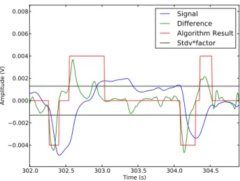
2.4 Algorithm process. The signal is represented in blue, the difference in green, the algorithm output in red and the standard deviation multiplied by a factor in black. . . 12

2.5 Supervised learning examples. Adapted from [3]. . . 14

2.6 Receiver Operating Characteristic (ROC) curve example, from [4]. . . 16

2.7 Classification for SVM(linear separable case). . . 17

3.1 Initial peak from the main device and its effect in the algorithm output.. . 22

3.2 Signal without the initial peak from the main device. . . 22

3.3 Artefacts of the main device or software with higher amplitude than the amplitude of the fish activity. . . 23

3.4 Artefacts of the main device, its effect in the algorithm result with and without the filter. Signal enhanced from 3.3.. . . 24

3.5 Platform Open Signals for synchronism between signal and video. . . 25

3.6 Abrupt tail-flip movement. . . 26

3.7 Visual analysis example. The signal is represented in blue and the be-haviour tail-flip detection in red. . . 27

3.8 User test. The signal is represented in blue, User 1 is represented in red and User 2 in green. The time interval accepted is in black. . . 28

(16)

xvi LIST OF FIGURES

3.10 Multiplicative factor effect over the algorithm output. Visual analysis is applied for each case in dotted lines to understand which multiplicative

factor is the most suited. . . 30

3.11 Relative error in percentage of the visual analysis and the algorithm output to understand which multiplicative factor is most suited for each group by minimizing its relative error. The black dotted lines represent the actual multiplicative factor (0.1), the red dotted lines the best multiplicative factor for treated fish and the blue dotted lines the best multiplicative factor for non-treated fish. . . 32

3.12 Relation between signal, visual analysis, and algorithm effect. The signal is represented in blue, the algorithm in cyan and the visual marks in red. . 32

4.1 Comparison between the visual analysis and the zero crossing rate param-eter. Linear regression is presented for each group and relative error was estimated with theleave one outmethod. . . 34

4.2 Classifier scheme in the Orange Software. . . 36

4.3 ROC curves and its convex curves for SVM (Green) and Naïve Bayes (Red) methods. Predicted class – "Healthy" . . . 38

4.4 Final algorithm process. . . 39

4.5 Open Signals with algorithm integration. . . 40

5.1 Intramuscular injection with 6-OHDA. . . 42

5.2 Behaviour results over the effect of 6-OHDA. The black bars represent mean±standard deviation. . . 43

(17)

List of Tables

2.1 Confusion Matrix. Tp andTn are the number of true and negative

exam-ples respectively. Fp andFn the number of false positives and negatives

respectively. . . 15

3.1 Specific values from figures 3.9, namely the visual analysis result and the

algorithm output using the actual multiplicative factor (0.1). . . 31

4.1 Confusion Matrix for each method used. Allows the comparison between

the predicted values and the correct class. . . 38

(18)

(19)

Acronyms

CNS Central Nervous System

DA Dopaminergic

DFT Discrete Fourier Transform

FFT Fast Fourier Transform

FPR False Positive Rate

hpf hours post-fertilization

IMM Instituto de Medicina Molecular

MFB Multispecies Freshwater Biomonitor

MOBS Marine On-line Biomonitor System

6-OHDA 6-hydroxydopamine

PD Parkinson’s Disease (Doença de Parkinson)

PSD Power Spectral Density

ROC Receiver Operating Characteristic

SVM Support Vector Machine

(20)

(21)

1

Introduction

1.1 Motivation

People are living longer. Since Parkinson’s Disease (PD) most commonly affects the el-derly, the number of sufferers will rise substantially in the years to come. The prevalence ofPDis1%to 2%of persons older than 60 years [5]. In turn, the need for clinical and social services to care for and support patients withPDwill increase at a rapid rate, with major implications for the resources that are allocated to healthcare [6].

There is currently no form of pharmacotherapy available that has shown to delay the progression ofPD. However, there are a range of drugs that can treat the symptoms of the condition and consequently improve the patient’s life quality. Also, the correct diag-nose ofPDespecially in the early stages of the disease, represent quite a challenge. PD

can cause a broad spectrum of symptoms and there are significant variations between patients in the way the disease manifests itself and the speed with which symptoms de-velop. However three symptoms are clearly fundamental: hypokinesia (reduction in movement), rigidity and tremor [6].

(22)

1. INTRODUCTION 1.2. Objectives

1.2 Objectives

The major aim of this work was the development of an algorithm that, once combined with theMOBSbiosensor, allows to differentiate electric signals between "healthy" and "ill" zebrafish and also provide its swimming activity in number of tail-flips per minute. Hence it will improve the detection of parkinsonism-like phenotypes in zebrafish.

1.3 Thesis Overview

The structure of this thesis is schematically represented in Figure1.1.

•1.Introduction

•2.Concepts

Basis

•3.Current Algortithm

Evaluation

•4.Proposed Algorithm

Developments

•5.Application

•6.Conclusions

Results

•Publication

Appendix

Figure 1.1: Thesis overview.

In the first two chapters the basis that support this research is reported. The motiva-tion and objectives are presented in Chapter 1. There was an initial effort to characterize the behaviour of zebrafish using an algorithm that provided the number of tail-flips per minute. Thus, the association between the zebrafish andPD, the current algorithm used to characterize the behaviour of zebrafish, as well as the description of the biosensor

MOBS are described in Chapter 2. In this chapter it is also reported machine learning techniques that were used in the implementation of the new algorithm.

Chapter 3 examines with more detail the current algorithm output using video, which required the development of a functionality in the platform Open Signals that allowed synchronism between video and signal. This detailed analysis demonstrated the need for creating a new algorithm that could simulate zebrafish behaviour as real as possi-ble. Chapter 4 presents the development of the new algorithm using machine learning techniques as well as its validation.

(23)

1. INTRODUCTION 1.3. Thesis Overview

contains the paper published in the context of this research work.

This thesis was written using the LA_{TEX environment [}₇_{]. The signal acquisition uses} the softwareMATLAB and the signal processing algorithms were developed inPython. The Orange software was used to build the classifier [8]. The final algorithm was also integrated in the platform Open Signals that required some knowledge inJavascriptand

HTML.

(24)

(25)

2

Concepts

2.1 Zebrafish and Parkinson’s Disease

2.1.1 Zebrafish

Zebrafish (scientific name -Danio rerio) are tropical fresh water fish from Ganges region of India. They can be found in Nepal, Bangladesh, Pakistan and Myanmar [9].

Figure 2.1: Zebrafish [1].

The fish seen in Figure 2.1 is named for the five horizontal blue stripes on the side of the body. Males are torpedo shaped and have gold stripes between the blue stripes; females have a larger, whitish belly and have silver stripes instead of gold. Fully grown adults are around 3-5 cm long and 1 cm wide.

(26)

2. CONCEPTS 2.1. Zebrafish and Parkinson’s Disease

2.1.2 Zebrafish as a model organism

Most insights into human disease are a result of experiments that would be unethical or unfeasible to perform on humans. Instead, biomedical research uses models to look at the functions of the genes involved in maintaining healthy organisms in order to obtain vital clues about the causes and progression of human diseases.

People are familiar with the use of mice and rats as model organisms (lab rats). As mammals they are very similar to humans, therefore they can be used to study complex processes underlying normal human development and diseases.

If we want to know something simple that is likely to occur in all living organisms than we can use bacteria or yeast as they are easy and cheap to look after and they’re very well understood. However, sometimes they can be too simple in terms of biological organization.

Zebrafish are the ideal model organism to bridge the gap between "too simple" and "too complex". They are aquatic vertebrates and have similar body plans (and similar tissues and organs) to humans, and they are much easier and with reduced cost to breed than mice and rats. Zebrafish has a short generation time (3 months) and breed prodi-giously (hundreds of offspring per female per week). They develop from a single cell in fertilized egg in about 24 hours (for a mouse it takes about 21 days). Also, the embryos are large, robust, transparent, easy to manipulate genetically and are developed outside the mother. Some drugs can even be administered by adding directly to the tank. Zebrafish mutations phenocopy many human disorders and the genome sequence of zebrafish is near completion [9].

However, besides all the advantages, zebrafish also have disadvantages when com-pared to other models. They are not mammals, so they are not as closely related to hu-mans as mice. Therefore, all the new discoveries must later be verified in a mammal model [10]. It is the similarity between the genes, which scientists call conservation, or genetic homology, the reason why fish can be used to study human diseases. Hence, ze-brafish can be used as a model organism.

The Central Nervous System (CNS) coordinates the activity of the body. It includes the brain and the spinal cord. Disorders in theCNScan affect control of physical move-ment, alteration of mood, change in sociability and absence of, or decline in communica-tion [9].

More and more groups are becoming interested in the fact that adult zebrafish pos-sess a high capacity for regeneration. Amazingly, spinal cord tissue can regenerate after a complete transection. In a process that takes about 6 weeks, approximately80%of ani-mals given a posterior injury achieve functional recovery [11]. This phenomenon is based on the striking ability of theCNSneurons to recover, traverse the lesion, and re-establish functional connections [12].

(27)

2. CONCEPTS 2.2. Marine On-line Biomonitor System –MOBS

Spastic Paraplegia, Parkinson’s Disease, Huntington’s Disease, Motor Neuron Disease and Multiple Sclerosis. These diseases cause loss of voluntary movement control in pa-tients. Given that their health is aggravated over time, they are called neurodegenerative disorders. At this moment there is no cure, and any treatment only slows the progression of symptoms [9].

2.1.3 Parkinson’s Disease

PD was first described in 1817 by James Parkinson and is the second most common neurodegenerative disorder, after Alzheimer’s disease [13]. ThePDis characterized by tremor, muscle rigidity, a slowing of physical movement, and can also cause cognitive and mood disturbances. It results of the loss of nerve cells in part of the brain known as the substantia nigra. These cells are called Dopaminergic (DA) neurons as they pro-duce the neurotransmitter - dopamine, which is used to send messages to the parts of the brain that co-ordinates movements. When around 80% of theDA neurons are lost, the symptoms ofPDstart to show. The cause ofPDis not absolutely clear; there are some mutations associated with the loss ofDA neurons and it is known that some toxins or chemicals may also cause the disease [9].

2.1.4 Parkinson’s Disease in Zebrafish

TheDAnervous system in zebrafish is well characterized in both embryos and adult ze-brafish. DAneurons are first detected between 18 and 19 hours post-fertilization (hpf). Some toxins known to induceDAcell loss in other animal models have now also been tested in adult zebrafish, as for example, the6-hydroxydopamine(6-OHDA) which is a neu-rotoxin that induces death of theDAcells [14,15,16]. The swimming velocity and total distance moved decreased after exposure to this neurotoxin [17,18]. Thus the evaluation of swimming behaviour can be related with the loss ofDAcells, and consequently with

PD.

2.2 Marine On-line Biomonitor System –

MOBS

A biosensor is defined as a self-contained integrated device that is capable of providing specific quantitative analytical information using a biological recognition element. The main advantages are the possibility of a continuous monitoring, the high specificity and sensitivity [19].

(28)

marine and fresh water species. This device was firstly applied successfully in the envi-ronmental field, and nowadays is used in the biomedical field, in particular, by sensing behavioural changes in organisms as an indication of stress or disease. Zebrafish has proved to be a suitable model candidate for this research since it has been used in medi-cal research during the past years, e.g in development studies [20], drug toxicity assess-ments [21] and neurodegenerative diseases [22]. Previous studies using this electronic device were used to asses water quality [2] and testing analgesics [23].

2.2.1 The main device

MOBSis an automatic system for recording behavioural responses of marine and fresh water species. Low power electrical signals are modulated by the behavioural activities of the organisms and then monitored, processed and analysed in real time.

The device monitors changes in electric fields caused by organism movements by means of non-invasive electrodes. It is an external automated transducer designed and manufactured at Faculty of Engineering of the University of Porto (Portugal). TheMOBS

device can record continuously specific behavioural activities of marine fish species, such as ventilation frequency and swimming activities and can quantify electrical signatures patterns from individual organisms as well as groups of animals.

Demodulation

Band-pass filtering

Fourier Transformation

Digital Signal

COMPUTER

Pre-amplification + mixing + Analogic to

Digital conversion Digital to Analogic

Convertion

Power Amplified

MOBS

Electric signals from the aquaria Electric signals to

the aquaria

CHAMBERS

Figure 2.2: The operation diagram of theMOBSsystem adapted from [2].

(29)

electrical signals into the water of the test chambers through a pair of non-invasive stain-less steel electrodes. The response is measured as a change in impedance of the water col-umn received by another pair of non-invasive stainless steel electrodes associated with movements of the fish [23]. The electrodes are attached vertically at the aquaria walls such that they provide a homogeneous distributed electric field across the entire aquar-ium.

The main device is controlled via an USB port by external processing software which produces signals in the digital domain (at 48000 samples/s or 48 kHz). These are con-verted by the main device into analogical electrical signals, power amplified and trans-mitted to the independent testing units at which they are conducted into the water by a pair of non-invasive stainless steel electrodes – Figure2.2. In response to the behavioural signatures of the organisms, the amplitudes of the electrical signals are modulated and then received by a second pair of electrodes. In the main device they are amplified and converted back to the digital domain at 48000 samples/s, before filtered, demodulated and down-sampled at 100 Hz by the external computer software. Then, they are anal-ysed in the frequency domain (Fourier transform with proper windowing) in chunks of about 10 s.

• Discrete Fourier Transform (DFT): The frequency domain allows a different vision

over the signal, and simplifies some operations like convolution and correlation. It is defined as:

Ar= N−1

X

k=0

Xkexp(−2jπrk/N) with r= 0,1, . . . , N −1 (2.1)

whereAris therthcoefficient of theDFTandXkdenotes thekthsample of the time

series which consists of N samples andj =√₋1. Also worth mentioning the Fast Fourier Transform (FFT) which is a method for efficiently computing the DFTof time series (discrete data samples)[24].

Upon processing, the system provides a signal in the frequency band of 0.2 Hz to 40 Hz that is correlated with the fish activity. As the harmonics are relevant to obtain signal shapes, they defined the cut-off frequency of the filters at around 45 Hz. This allows to obtain a clear representation of the direct time domain signal and its frequency spectrum, which is suitable to broaden the range of pattern recognition algorithms that can be used afterwards [2].

2.2.2 Other biosensor

(30)

2. CONCEPTS 2.3. Behaviour in Zebrafish

several kinds of freshwater organisms, mainly to test behavioural effects to the exposure of pharmaceutical effluents and to pollution detection on aquatic invertebrates and fish. These studies were analysed using theFFT[25,26].

Yet one of the advantages from this biosensor related toMOBSis the fact that in order to prevent the organisms from touching the electrodes, the chambers walls are covered with nylon netting (50µm) [27].

2.3 Behaviour in Zebrafish

Behaviour is the final outcome of a sequence of neurophysiological events including stim-ulation of sensory and motor neurons, muscular contractions, and release of chemical messages [27]. On-line biomonitors frequently use behaviour as an end point, which pro-vides a visual and, thus, measurable response at the whole-organism level. This method generates fast and sensitive results that can be integrated in many biological functions [28].

There is a lack of studies on complex behaviour in zebrafish; although it is recognised as having great potential as a model for understanding the genetic basis of human be-havioural disorders. One area of interest has been the effect of drugs on behaviour and also the studying of social behaviour, learning and memory.

The number of behavioural studies of zebrafish looks set to increase, and many re-searchers whose primary expertise is in genetics or development biology are using be-havioural protocols as a paradigm for testing the reinforcing properties of drugs of abuse. One of the problems with designing and conducting behavioural experiments is demon-strating that the results are a valid measure of the behaviour under consideration. Thus there is a need for adequate controls, in order to ensure that the results are not due to unrelated artefacts, for example, outside disturbance, either visual or auditory and accli-matisation. The behaviour may also vary according to the time of the day at which ob-servations are recorded, especially in relation to matting behaviour and feeding regime [15]. The next subsections describe the behaviour studied withMOBS.

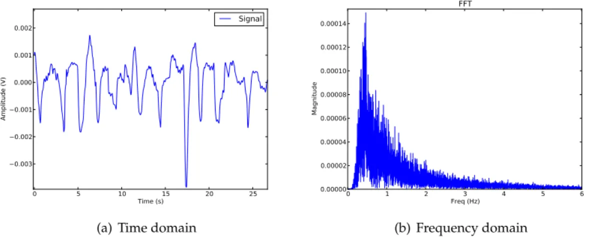
2.3.1 Locomotion

A typical activity using zebrafish in the time domain ofMOBSis shown in Figure2.3(a). The amplitude of the fish activity in the time domain is in the order of the mV.

(31)

2. CONCEPTS 2.4. Current Algorithm

0 5 10 _{Time (s)}15 20 25

0.003 0.002 0.001 0.000 0.001 0.002 Amplitude (V) Signal

(a) Time domain

0 1 2 3 4 5 6

Freq (Hz) 0.00000 0.00002 0.00004 0.00006 0.00008 0.00010 0.00012 0.00014 Magnitude FFT

(b) Frequency domain

Figure 2.3: Locomotion of a "healthy" fish represented in time and frequency domain (as "healthy" is meant that is neither "ill" nor transgenic).

2.3.2 Ventilation

Ventilation consists in opening and closing of mouth/operculum and causes only very local disturbances in the water. The smaller the distance between electrodes and organ-ism, the better the corresponding electric field can be identified and quantified. Typically ventilation generates waves of triangular shape with a higher frequency and smaller am-plitude than most of the energy located for locomotion. Ventilation can be detected and quantified by frequencies and thus requires a clear peak in the frequency spectrum [2]. However, ventilation will not be studied with zebrafish given its high level of activity.

2.4 Current Algorithm

An algorithm is a sequence of instructions designed to solve a problem [29]. The current algorithm used to characterize the behaviour of zebrafish consists in the evaluation of a specific locomotion behaviour of zebrafish, with a series of bursts in the domain ofMOBS

corresponding to the zebrafish tail-flip activity. Thus the outcome reflects the number of tail-flips per minute per individual fish [23].

The algorithm process uses the derivative of the signal in the time domain. This will allow the detection of the behaviour tail-flip, with representative peaks of the derivative that characterize the strong bursts. These peaks are detected using the standard deviation of the signal multiplied by a factor, to allow the comparison between the two parameters standard deviation and derivative, given that, the behaviour tail-flip can be detected. However, this algorithm detection compared with the actual fish behaviour requires con-firmation, and this can be accomplished by using video synchronized with the signal in the time domain.

(32)

2. CONCEPTS 2.4. Current Algorithm

Figure2.4presents an example of a "healthy" fish behaviour associated with its deriva-tive. The fish strong bursts result in signal (blue) variations and consequently provide defined peaks of the difference (green). Thus the algorithm output (red) will detect these peaks using a threshold that is defined by the standard deviation multiplied by a fac-tor (black). To refer that the difference, the standard deviation and the algorithm output were amplified in this case to simplify visualization.

302.0 302.5 303.0 303.5 304.0 304.5

Time (s) 0.004

0.002 0.000 0.002 0.004 0.006 0.008

Amplitude (V)

Signal Difference Algorithm Result Stdv*factor

Figure 2.4: Algorithm process. The signal is represented in blue, the difference in green, the algorithm output in red and the standard deviation multiplied by a factor in black.

For an easy behaviour analysis, the algorithm is created with -1, 0 and 1 values as seen in Figure 2.4(red). The values -1 and 1 are attributed if the difference exceeds the standard deviation, and passes to 0 when the difference is null. The 0 value is maintained until the difference exceeds again the standard deviation. Finally the algorithm will count the number of resulting transitions 0/1, 0/-1 and divide it by the total time of the signal in minutes providing the number of tail-flips per minute, of an individual fish.

2.4.1 Need for improvement

The pre-defined thresholds (multiplicative factor, maximum and minimum amplitude for the fish activity) are one of the reasons for confirmation and improvement. The algorithm only provides one type of behaviour, the tail-flips, which is a measurement of the fish activity (the higher the number of tail-flips, the more active the fish is). Nevertheless the possibility to study other behaviour (e.g. swimming and ventilation) may turn this algorithm more advantageous and complete for future works.

A more detailed analysis in the signal compared to the actual fish behaviour is nec-essary, which requires synchronism between signal and video. Possible errors from the main device that are visible in the signal need to be detected and filtered.

(33)

2. CONCEPTS 2.5. Machine Learning

was developed to study theDAneurons. This transgenic line was treated with the neu-rotoxin6-OHDAand behavioural effects investigated with theMOBSbiosensor. It was demonstrated that the drug induces behavioural changes that were related to the death ofDAneurons. The use of an improved algorithm could contribute as a more sensitive tool in the detection of behavioural phenotypes associated with the loss of theDA neu-rons. Thus it is essential to confirm if the actual algorithm is in fact detecting the right behaviour - the tail-flips. To develop a new algorithm, Machine Learning techniques are suggested.

2.5 Machine Learning

Machine Learning enables the extraction of implicit, previous unknown, and potentially useful information from data [30].

By Arthur Samuel (1959), machine learning is the field of study that gives computers the ability to learn without being explicitly programmed. A more recent definition by Tom Mitchell (1998) says: "A computer program is said to learn from experienceEwith respect to some taskT and some performance measureP, if its performance onT, as measured byP, improves with experienceE" [3].

Machine learning is used do extract information from the raw data in databases -information that is expressed in a comprehensible form and can be used for a variety of purposes. The process is one of abstraction: taking the data, warts and all, and inferring whatever structure underlies it. With machine learning we can use tools and techniques that are used for finding, and describing, structural patterns in data [30].

There are different types of machine learning algorithms, the main two types are: unsupervised and supervised learning.

2.5.1 Unsupervised Learning

With unsupervised learning it is intended to let the computer learn by it self. The right answers are not labelled in the data, there is no such supervisor and there is only input data. Finding some structure is possible using clustering algorithms which allows groups separations [3,31].

2.5.2 Supervised Learning

(34)

0 1 2 3 4 5 6 7

Size 0 1 2 3 4 5 6 7 Price Housing Price Linear Regression

(a) Linear Regression

0 1 2 3_{Tumor Size}4 5 6 7 0.5

0.0 0.5 1.0 1.5

Benign - 0, Malignant - 1

(b) Classification

0 1 2 3_{Tumor Size}4 5 6 7 0 1 2 3 4 5 6 7 Age Linear Regression

(c) Classification using two input variables. Blue represents benign tumor and green malignant tumor.

Figure 2.5: Supervised learning examples. Adapted from [3].

2.5.2.1 Regression Problems

Predict continuous valued output, for example predict the price of a house according to its size using linear regression - Figure2.5(a). In cases where the linear model is too restrictive, one can use for example a quadratic or a higher-order polynomial, or any other non-linear function of the input, this time optimizing its parameters for best fit.

Given a training set withmtraining examples we can representxas the input vari-able/feature,yas the output variable or target variable andhθ(x)our hypothesis which

estimates the outputy. It is used to make predictions. Related to Figure2.5(a)17 train-ing examples are used, with the size of the house as the input variable and the price as output.

Linear Regression

When the output and all input variables are numeric, linear regression is a natural tech-nique to consider. Also when using more than one variable it is important to consider that there might be a single variable that does all the work and the others are irrelevant or redundant.

The hypothesis using one input variable as seen in Figure2.5(a)can be expressed as:

hθ(x) =θ0+θ1x (2.2)

Whereθ0 andθ1 are the parameters used so thathθ(x)is close to the outputy when

using our training examples. Here, the machine learning program optimizes the param-eters, θ, such that the approximation error is minimized, that is, our estimates are as close as possible to the correct values given in the training set. In many cases, there is no analytical solution and we need to resort to iterative optimization methods. The most commonly used are gradient descent and normal equation [31].

(35)

2.5.2.2 Classification problems

This technique intends to predict discrete valued outputs, for example predict if a tumour is benign or malign according to the tumour size – Figure2.5(b). It is also possible to use more than one input variable to predict the output as seen in Figure2.5(c), which uses two input variables, the tumor size and age, to classify if the tumor is benign or malignant.

Classification problems can use two classes (e.g predict if a tumor is benign or malig-nant), or multi-classes. From figures2.5(b)and2.5(c), the aim is to infer a general rule, coding the association between the input attributes and its output. That is, the machine learning system fits a model to the past data to be able to estimate the tumor malignancy for a new situation [3,31]. Using two classes it is important that our hypothesis is given in terms of probability, so that the class that presents higher probability will be chosen.

Classification Performance

The data produced by a classification scheme during testing are counts of the correct and incorrect classifications from each class. This information is then normally displayed in a confusion matrix - Table2.1.

Table 2.1: Confusion Matrix. Tp andTn are the number of true and negative examples

respectively.FpandFnthe number of false positives and negatives respectively.

C or rect C la ss Healthy Sick Sum Predictions Healthy Tp Fp Tp+Fp Sick Fn Tn Fn+Tn Sum

Tp+Fn

Fp+Tn

Tp+Fn+ Fp+Tn

A confusion matrix is a form of contingency table showing the differences between the true and predicted classes for a set of labelled examples. ConsideringTp andTnthe

number of true positives and true negatives respectively,Fp andFnthe number of false

positives and negatives respectively, there are measures that can be extracted from the confusion matrix:

Accuracy = Tp+Tn

Tp+Fp+Tn+Fn (2.3)

Sensitivity = Tp

Tp+Fn (2.4)

Specif icity= Tn

Tn+Fp (2.5)

(36)

applied. The accuracy from equation2.3is the proportion of correctly classified examples among all data classified. The sensitivity - equation 2.4, also called True Positive Rate (TPR) is the number of detected positive examples among all positive examples, e.g. the proportion of healthy people correctly diagnosed as healthy. The specificity - equation

2.5, is the proportion of detected negative examples among all negative examples, e.g. the proportion of sick correctly recognized as sick [8]. A good way of visualising a classifier’s performance is with the Receiver Operating Characteristic (ROC) curve – Figure2.6.

Figure 2.6:ROCcurve example, from [4].

It consists in plotting the sensitivity according to the False Positive Rate (FPR) (1-specificity) for different cut-off points of a parameter [32]. Each point on theROCcurve represents a sensitivity/specificity pair corresponding to a particular decision threshold. The ROC curve shows how the number of correctly classified positive examples varies with the number of incorrectly classified negative examples [33]. A test with perfect dis-crimination (no overlap in the two distributions) has aROC curve that passes through the upper left corner (100% sensitivity, 100% specificity). Therefore the closer the ROC

curve is to the upper left corner, the higher the overall accuracy of the test [34].

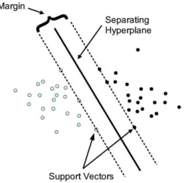
A possible classifier is the Support Vector Machine (SVM), a powerful technique for general (non-linear) classification, regression and outlier detection with an intuitive model representation. SVMwas developed by Cortes and Vapnik (1995) for binary clas-sification. Their approach may be roughly sketched as follows:

• Class separation: basically, we are looking for the optimal separating hyper-plane

between the two classes by maximizing themarginbetween the classes closest points (Figure 2.7)- the points lying on the boundaries are calledsupport vectors, and the middle of the margin is our optimal separating hyperplane;

(37)

are weighted down to reduce their influence;

• Non-linearity: when we cannot find a linear separator, data points are projected

into an (usually) higher-dimensional space where the data points effectively be-come linearly separable (this projection is accomplished via kernel techniques);

• Problem solution: the whole task can be formulated as a quadratic optimization

problem which can be solved by known techniques.

Figure 2.7: Classification forSVM(linear separable case).

An algorithm able to perform all these tasks is called aSupport vector machine[35]. There are at least three reasons for the success of theSVM: its ability to learn well with only a very small number of free parameters, its robustness against several types of model violations and outliers, and last but not least its computational efficiency compared with several other methods (e.g. Logistic regression) [36]. As for disadvantages, if the number of features is much greater than the number of samples, the method is likely to give poor performance. Also SVM do not directly provide probability estimates, these are calculated using five-fold cross-validation, and thus performance may suffer [37].

Besides SVM another method that is very used in classification is the Naïve Bayes classifier. Naïve Bayes classifier is a supervised learning algorithm based on applying Bayes theorem with the "naïve" assumption of independence between every pair of fea-tures. Bayes’ rule says that if you have a hypothesisHand evidenceEthat bears on that hypothesis, then:

P[H_|E] = P[E|H]P[H]

P[E] (2.6)

(38)

these pieces of evidence are independent (given the class), their combined probability is obtained by multiplying the probabilities:

P[H_|E] = P[E1|H]×P[E2|H]×...×P[En|H]×P[H]

P[E] (2.7)

This method goes by the name of Naïve Bayes because it is based on Bayes’ rule and "naïvely" assumes independence [30]. These classifiers have worked quite well in many real-world situations, such as document classification and spam filtering. They require a small amount of training data to estimate the necessary parameters.

Naïve Bayes classifiers can be extremely fast compared to more sophisticated meth-ods. The decoupling of the class conditional feature distributions means that each dis-tribution can be independently estimated as a one dimensional disdis-tribution. In turn this helps to alleviate problems stemming from the curse of dimensionality [38]. However, there are many datasets for which Naïve Bayes does not do well. Because attributes are treated as though they were independent given the class, the addition of redundant ones skews the learning process [30].

2.5.3 Feature Extraction

There are many features/parameters that can be used as input variables in our prob-lem. Besides the current algorithm output in section2.4the following features were also computed:

• Zero Crossing Rate – It is defined as the number of time-domain zero crossings

within a defined region of signal, divided by the number of samples of that region [39]. The zero crossing process consists in counting the number of times that the signal changes sign, meaning, it counts when the signal passes from negative to positive and from positive to negative.

• Standard Deviation – The standard deviation is equal to the square root of the

variance and measures how much variation exists from the signal average. A small value of standard deviation indicates that the points tend to be very close to the average, whereas a high value that the points are very spread out and more apart from the average. Considering a signal defined over a finite time window with length N, and represented as time series [x(n)], the standard deviationσ can be represented using the averageµ[40]:

σ = v u u t1 N

N−1

X

n=0

[x(n)₋µ]2

where µ= 1 N

N−1

X

n=0

[x(n)] (2.8)

• Histogram– Given an univariate sampleS=x1, x2, ...xn, this one can be processed

(39)

χbe the set of possible distinct values inS. For eachx_∈χthe relative frequency is:

f(x) = the number of xi ∈S for which xi =x

n (2.9)

A discrete-data histogram is a graphical display of the relative frequency where each distinct value in the sample appears [41]. One possible parameter to extract from the histogram is the maximum number of occurrences which represents the maximum value of the numerator in equation2.9.

• Periodogram – Is based on the definition of the Power Spectral Density (PSD) as

seen in equation2.10. One of the first uses of thePSD, has been in determining possible "hidden periodicities" in time series, which may be seen as a motivation for the name of this method [42,43]. A possible parameter to extract from thePSD

is the maximum power spectral density which represents the maximum value from equation2.10.

Pxx(f) =

1 N|

N−1

X

k=0

Xkexp(−2jπrk/N)|

2

(2.10)

whereN is the number of examples, and

N−1

P

k=0

Xkexp(−2jπrk/N)theDFTalready

defined in equation2.1.

2.5.4 Performance Measures

Performance tests are used to validate machine learning models and algorithms. A pos-sible statistical test isleave one out; for a given dataset ofminstances, only one instance is left out as the validation set (instance) and training uses them₋1instances. We then getmseparate pairs by leaving out a different instance at each iteration. The results of allm judgements, one for each member of the dataset, are averaged, and that average represents the final error estimate.

This procedure is an attractive one for two reasons. First, the greatest possible amount of data is used for training in each case, which presumably increases the chance that the classifier is an accurate one. Second, the procedure is deterministic: no random sampling is involved. There is no point in repeating it 10 times, or repeating it at all: the same result will be obtained each time. Set against this is the high computational cost, because the entire learning procedure must be executed m times and this is usually infeasible for large datasets. Nevertheless, leave-one-outseems to offer a chance of squeezing the maximum out of a small dataset and getting as accurate an estimate as possible [30,31].

(40)

Often in the study of behavioural ecology, and more widely in science, we require to statistically test whether the central tendencies (mean or median) of 2 groups are different from each other on the basis of samples of the 2 groups [45].

(41)

3

Current Algorithm Evaluation

In this chapter the data improvements ofMOBSbefore applying the current algorithm are presented. The zebrafish behaviour are analysed using the platform Open Signals that will enable synchronism between video and signal. The thresholds used in the current algorithm are also tested and new suggestions are made regarding the usefulness of the algorithm.

3.1 Preparing the Data

3.1.1 Start Peak

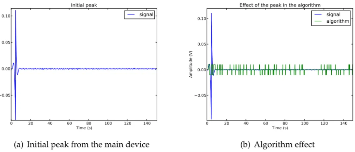
After starting the main device to visualize the fish locomotion, it is noticed in the time domain, an initial peak of higher amplitude than the fish activity. This peak is charac-teristic of the main device. Following this peak the fish activity is measured. The delay from the main device until the fish activity is displayed is approximately 30 seconds, and considering this, the current algorithm contained only the analysis of the signal after 30 seconds. However it was noticed that the peak was still present - Figure3.1(a). The presence of this peak certainly changes the algorithm output as seen in Figure3.1(b).

This situation was solved by using the algorithm furthermore in the signal. Given that, instead of considering30seconds before the analysis, the algorithm only acts in the signal after40seconds. This guarantees that the initial peak is not presented, and that the evaluation of the algorithm is not corrupted by this peak. The result is shown in Figure

3.2.

(42)

3. CURRENTALGORITHMEVALUATION 3.1. Preparing the Data

0 20 40 60 _{Time (s)}80 100 120 140

0.05 0.00 0.05 0.10

Amplitude (V)

Initial peak

signal

(a) Initial peak from the main device

0 20 40 60 _{Time (s)}80 100 120 140

0.05 0.00 0.05 0.10

Amplitude (V)

Effect of the peak in the algorithm signal algorithm

(b) Algorithm effect

Figure 3.1: Initial peak from the main device and its effect in the algorithm output.

0 10 20 30 40 50 60

Time (s) 0.002

0.001 0.000 0.001 0.002 0.003

Amplitude (V)

Activity without initial peak

Figure 3.2: Signal without the initial peak from the main device.

• Increase of the algorithm output - tail-flips per minute. This situation happens due to the standard deviation that decreases because of the absence of the initial peak. Given that, more peaks from the derivative will be detected as tail-flips. It is important then to ascertain that the threshold used to allow the behaviour detection in the algorithm, the multiplicative factor (see section2.4), is in fact the correct one to detect the tail-flips.

• Decrease of the algorithm output - tail-flips per minute. This happens because the transitions detected by the algorithm from this initial peak are no longer counted -Figure3.1(b). Consequently the number of tail-flips decreases.

(43)

3. CURRENTALGORITHMEVALUATION 3.1. Preparing the Data

greater importance the absence of this peak in the algorithm evaluation.

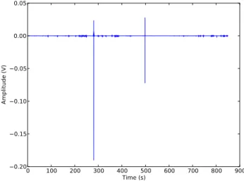
3.1.2 Error Peaks Detection

Another difficulty related to the main device occurs during the recording of the fish activ-ity. It was noticed in the time domain the presence of peaks with much higher amplitude than the fish activity - Figure3.3.

0 100 200 300 400 500 600 700 800 900

Time (s) 0.20

0.15 0.10 0.05 0.00 0.05

Amplitude (V)

Figure 3.3: Artefacts of the main device or software with higher amplitude than the am-plitude of the fish activity.

Since we can record more than one chamber at the same time, it was possible to visu-ally identify these peaks in each chamber at the same time. Given that, we can say that the problem was not from one chamber in particular, but from the main device itself or from the computer software. The impact of these peaks on the results is well noticed in Figure3.4(a).

The idea to solve this problem was by the application of a filter. The fact that this peak is of higher amplitude than the fish activity, turns it easy to identify. Then for the filter process, it is used 0 values when those peaks are detected and 1 values otherwise. In the end the filter is multiplied with the signal to exclude these peaks for further analysis. The filter result is shown in Figure3.4(b).

(44)

3. CURRENTALGORITHMEVALUATION 3.2. Synchronism

280.4 280.6 280.8_{Time (s)} 281.0 281.2 281.4 0.004 0.002 0.000 0.002 0.004 0.006 0.008 Amplitude Signal Difference Algorithm Result Stdv*factor

(a) Algorithm effect

280.2 280.4 280.6 280.8_{Time (s)}281.0 281.2 281.4 0.000 0.005 0.010 Amplitude Signal Difference Algorithm Result Filter Stdv*factor

(b) Algorithm with filter

Figure 3.4: Artefacts of the main device, its effect in the algorithm result with and without the filter. Signal enhanced from3.3.

3.2 Synchronism

The signal in the time domain is delayed in relation to the instant of acquisition start. This delay is caused by the main device. Given that, it is difficult to compare a video where the fish movements are present, with its respective signal fromMOBS.

3.2.1 Open Signals

The Open Signals is a platform designed and programmed byPLUX - Wireless Biosignals, S. A. It is a useful tool for this research, because it will allow synchronism between signal and video.

Using Open Signals, synchronism is possible with a visible stimulus in the signal and video. This stimulus must be sufficient to not be confused with the fish activity as shown in Figure3.5. A touch in the chamber is a possible stimulus and to not corrupt the signal from the fish activity for further analysis, this stimulus should be produced at the end of the recording.

With this platform, the user can navigate freely through the signal and video inde-pendently (without both being synchronized yet). The synchronism is accepted after the user locks both signal directly in the window and video using the lock button (Figure

3.5). After the right time is selected in accordance to the stimulus made, it will be pos-sible to analyse the signal variations in comparison to the fish movements in the video. Navigating in one datum will automatically progress the other in the same way allowing the study of their behaviour more precisely.

3.2.2 Time Precision

(45)

Figure 3.5: Platform Open Signals for synchronism between signal and video.

minutes with the empty chamber submersed in water. In this 30 minutes several stimuli were made in the chamber and recorded in video. After synchronism it was verified that each stimulus in the signal corresponded at the same moment in the video (variation of 0.13_±0.05seconds between the stimulus identified in the signal and video).

Hence, it is possible to make behavioural tests for 30 minutes efficiently since for at least this length of time we know that the main device is precise.

3.2.3 Experimental Design

This subsection presents the experimental design performed with zebrafish. These tests will allow the study of their behaviour using the synchronism between video and signal. Since the drug that simulatesPDleads to a decrease in the fish activity [17,18], it is also intended to analyse by eye the tail-flip movements when the fish are submitted to the

drug6-OHDA.

3.2.3.1 Test Animals and6-OHDA

The zebrafish (D. rerio Hamilton 1822) strain used for this work was the AB line (Ze-brafish Facility, IMM, Portugal). Animals were maintained under standard conditions and experiments were approved by the Institutional Animal Care and Use Committee. A master stock solution of 6-hydroxydopamine hydrochloride (6-OHDA, Sigma-Aldrich, USA) was prepared in0.2%ascorbic acid solution (analytical grade, Sigma) and stored at -20◦_{C. This stock solution was used to prepare all working solutions in experiments with}

(46)

3.2.3.2 Behaviour Assay

Before the experiments, small groups of female fish (24 animals, body weight 0.5±0.05 g) were acclimatized to the experimental testing conditions (temperature 22◦_C_±₁◦_C,

10 h:12 h light-dark cycle) in 17 litre glass aquaria under static conditions and for a min-imum of one week. Food was not provided 24 h before or during the experiments. The behaviour analysis was divided into two groups: non-treated (12 fish) and for that con-sidered as "healthy" fish in which no injection was administered, and treated (12 fish) also considered as "ill" or less active where5µLof 6-OHDAwas injected via intramus-cular. During the injection they were in a medium-to deep-plane level of anaesthesia (tricaine50mg/L) and had lost their reflex responses and muscular control. Afterwards they returned to their original test chambers and allowed 30 min to recover from the anaesthesia.

On the day of experiments, either the treated or non-treated groups of fish were placed individually in the test chambers supplied with oxygenated tap water (22◦_C_±₁ ◦_{C). Fish were acclimated to the test chambers for 30 min and then individual baseline}

responses were monitored using MOBSand video recording (at 25 frames per second) for five minutes between 10 and 12 a.m.

After behavioural recording, treated fish were sacrificed with tricaine. The behavioural experiments were always performed by the same experimenter.

3.2.3.3 Behaviour Detection

Using video recording it is possible to distinguish tail-flip movements. This behaviour is characterized by abrupt and fast changes of fish direction which imply strong burst in the fish tail (Figure3.6).

Figure 3.6: Abrupt tail-flip movement.

3.2.4 Visual Analysis

A visual and detailed analysis was made with the Open Signals platform using video frame by frame with both signals synchronised taken in consideration the behaviour tail-flip.

(47)

the detections, this information was saved in a file in the following order: time; signal; behaviour detection. The result is presented in Figure3.7.

65 66 67 68 69 70 71

Time (s) 0.0004

0.0002 0.0000 0.0002 0.0004 0.0006 0.0008

Amplitude (V)

Signal Abrupt Flip-tail

Figure 3.7: Visual analysis example. The signal is represented in blue and the behaviour tail-flip detection in red.

Since the actual algorithm output returns the number of abrupt tail-flips per minute, we can now compare it with the visual analysis. The process is as simple as count the number of abrupt tail-flips visually detected in the created file and divide it by the total signal time in minutes. Then compare it with the value of the algorithm output. This may bring an idea of how far we are from reality.

3.2.5 User Test/Visual Analysis Validation

Since visual analysis depends on the user that is interpreting the data, it is important to test other users and compare the results. Therefore, a visual test using a different user was made, providing only the description and images explained in section3.2.3.3. Figure

3.8shows the detection for both users.

The test consisted in a precise analysis frame by frame using a signal of 30 seconds, and for this time both users detected 46 abrupt tail-flips. After User 1 had detected the abrupt tail-flip it was considered an interval of0.25seconds in which the User 2 had also to detect the same abrupt tail-flip to be a valid success. Given that, in 46 detections, 44 were accepted, leading to an error of4.35%between both users.

(48)

3. CURRENTALGORITHMEVALUATION 3.3. Thresholds

21.0 21.5 22.0 22.5 _{Time (s)}23.0 23.5 24.0 24.5 0.003

0.002 0.001 0.000 0.001 0.002 0.003 0.004

Amplitude (V)

User 1 User 2 Time Interval

Figure 3.8: User test. The signal is represented in blue, User 1 is represented in red and User 2 in green. The time interval accepted is in black.

3.3 Thresholds

This section will allow an improvement in the thresholds already implemented in the current algorithm, specifically in the maximum and minimum amplitude accepted for the fish activity. The multiplicative factor is analysed in the next section. Several tests were performed and based on the results, new considerations were made, as following:

• Minimum Amplitude– The threshold used to limit the minimum amplitude for

the fish activity and therefore the maximum amplitude for the noise is 0.5 mV. Tests without fish and with the chambers submersed in the water were performed. Af-terwards the maximum amplitude for each test was measured. The maximum am-plitude encountered was 0.6 mV, leading to a variation of 0.1 mV from the previous threshold.

• Maximum Amplitude – The threshold used to limit the maximum amplitude of

the fish activity is 0.01 V. Tests performed with fish, showed that the maximum amplitude measured from all chambers was the same. Given that, no change was made.

3.4 Algorithm Evaluation

This section intends to compare the visual analysis with the algorithm output. The result is shown in Figure 3.9where linear regression was applied for each group (treated and non-treated).

(49)

3. CURRENTALGORITHMEVALUATION 3.4. Algorithm Evaluation

0 20 40 _{Algorithm Result tail-flips/min}60 80 100 120 140 160 0

10 20 30 40 50 60 70 80 90

Visual Analysis tail-flips/min

Healthy Ill/Less Active

Figure 3.9: Comparison between the visual analysis and the algorithm output both in number of tail-flips per minute. Linear regression is presented for each group and relative error was estimated with theleave one outmethod.

subsections demonstrate the validation for each group and the error associated will show the need for improvement in the current algorithm, concretely in the multiplicative factor.

3.4.1 Validation for healthy fish

For validation it the statistic method leave one outwas used. This was chosen because the number of points analysed is small (n = 12). The process was: take one point out, obtain the linear regression with all the others points, and measure the expected tail-flips of the point that was excluded using the calculated linear regression. The relative error of the respective point consists in the difference of its real value (the tail-flips obtained visually) with the expected value divided by the real value. Then it is necessary to repeat this process to all points, meaning, there will be as much relative errors as the numbers of points used. In the end, all relative errors are averaged. The non-treated group has a relative error of17.29%using a window of 180 seconds (Figure3.9) and a correlation coefficient of0.015. More points can be provided with the usage of a smaller window, and this was accomplished using windows of 60 seconds which resulted in an error of 19.34%and a correlation coefficient of0.014. Given that the relative error is higher, the validation will use the analysis for a window of 180 seconds.

3.4.2 Validation for ill fish

(50)

3.4.3 Multiplicative factor

The multiplicative factor in the algorithm is used so that the derivative can be comparable to the standard deviation thus allowing the behaviour tail-flip to be detected. Given that, to improve the algorithm, the multiplicative factor should be analysed. Also, after the studies made in the previous sections, it was said that this factor needed verification (see section3.1). The value used so far has been0.1. To facilitate we vary the factor according to the algorithm output as shown in figures 3.10and compare it with the visual result. The factor is analysed from0to0.25with a variation of0.01.

0.05 0.10_Factor 0.15 0.20

0 20 40 60 80 100 120 140

Algorithm Result (tail-flips/min)

Non-Treated Fishes

Actual Threshold Visual Counts

(a) Non-treated fish group.

0.000 0.05 0.10_Factor 0.15 0.20

20 40 60 80 100 120 140

Algorithm Result (tail-flips/min)

Treated Fishes

Actual Threshold Visual Counts

(b) Treated fish group.

Figure 3.10: Multiplicative factor effect over the algorithm output. Visual analysis is applied for each case in dotted lines to understand which multiplicative factor is the most suited.

Focusing on a particular case (red analysis in Figure3.10(a)) it is visible that the actual threshold used (0.1) leaded to a result that was different from the visual analysis, indicat-ing that in this case, the factor that should be used is not0.1but in fact0.08approximately. With the analysis of more cases, it was expected to find an approximate factor value for all cases or a direct association. Unfortunately this did not happen either for non-treated and treated groups, in that, there are different factors that suit the actual algorithm ac-cording to each case. However it is visible that if there is an ideal multiplicative factor, the one should probably be between0and0.25.

To reinforce this study, table3.1 demonstrates the specific values obtained for each group. In these tables the visual results obtained are shown as well as the algorithm out-put using the current multiplicative factor (0.1). These tables demonstrate that there are substantial differences between the visual analysis and the algorithm output.

The intention of the next analysis is to be able to understand which multiplicative factor is the most suited to be used for the detection of the behaviour tail-flip and its respective relative error. The process was to subtract each value of the curves in figures

(51)

Table 3.1: Specific values from figures3.9, namely the visual analysis result and the algo-rithm output using the actual multiplicative factor (0.1).

(a) Non-treated fish group

Visual Result (tail-flip/min) 40.67 47 47.667 51.67 52.333 56.333 58 62 64.333 64.333 69 80 Algorithm Output (tail-flip/min) 38.980 8.993 35.97 56.133 58.768 86.044 63.653 6.295 126.144 12.332 142.191 21.324

(b) Treated fish group

Visual Result (tail-flip/min) 11.333 14.333 15 18.667 26.333 27.333 28 29.333 31.333 31.667 35.333 36.667 Algorithm Output (tail-flip/min) 0.654 24.143 0 0 0 50.401 49.853 48.559 48.976 45.497 37.639 47.252

error. In the end all curves analysed are averaged and the result is shown in Figure3.11

for each group. Here is presented the minimum error accepted as well as the error used with the actual factor for each group.

The error using the actual factor is 55.26% and 68.79% for non-treated and treated groups respectively, and even improving the factor, the minimum error accepted would be53.20%for non-treated group which leads to a best factor of0.11and44.53%for treated group with a best factor of0.13. To be able to choose the best factor these obtained errors should be as close to zero as possible which indicates that even with these improvements the best multiplicative factor cannot be certain to characterize the behaviour as close to reality as it is pretended.

Because the user analysis has already been tested, and thus, considering that the vi-sual analysis is a valid measure, there are two possible reasons to explain these high errors: the algorithm or the biosensorMOBS.

3.4.3.1 Algorithm Insight

The algorithm output consists in the peaks detection of the derivative using a given threshold so that the behaviour tail-flip can be detected. This threshold is represented by the standard deviation with a multiplicative factor so that the standard deviation may be comparable with the derivative.

The main problem verified is that the abrupt tail-flips detected visually do not always show the same characteristic in the signal, and consequently, an abrupt tail-flip detected visually not always imply a representative peak in the derivative. Figure3.12(a)shows that case.

(52)

0.00 0.05 0.10 0.15 0.20

Factor 0 20 40 60 80 100 120 140

Relative Error (%)

Non-treated Treated

Figure 3.11: Relative error in percentage of the visual analysis and the algorithm output to understand which multiplicative factor is most suited for each group by minimizing its relative error. The black dotted lines represent the actual multiplicative factor (0.1), the red dotted lines the best multiplicative factor for treated fish and the blue dotted lines the best multiplicative factor for non-treated fish.

191 192 193 _{Time (s)}194 195 196 197

0.004 0.002 0.000 0.002 0.004 Amplitude (V) Signal Algorithm Result Abrupt Flip-tail

(a) Behaviour detection visually identified but not from the algorithm.

90 91 92 93_{Time (s)}94 95 96 97 98

0.004 0.002 0.000 0.002 0.004 Amplitude (V) Signal Algorithm Result Abrupt Flip-tail

(b) Behaviour detection from the algorithm but not visually identified.

Figure 3.12: Relation between signal, visual analysis, and algorithm effect. The signal is represented in blue, the algorithm in cyan and the visual marks in red.

Therefore it is suggested the development of a new algorithm that can characterize the behaviour as close to reality as possible.

3.4.3.2 BiosensorMOBS

(53)

4

Proposed Algorithm

In this chapter new parameters are discussed to characterize the abrupt tail-flip move-ments. With the visual analysis obtained from the previous chapter it will be possible to study new parameters using supervised learning methods, more precisely, regres-sion models. Thus our visual analysis will be considered as the output variable, and the new parameters the input variables. It is also shown the need for classification between "healthy" and "ill" fish. Finally, a new algorithm is proposed as well as its integration in the Open Signals platform.

4.1 Behaviour Characterization

To be able to characterize the behaviour in number of tail-flips per minute, the param-eter zero crossing rate proved to be useful. This paramparam-eter is defined as the number of time-domain zero crossings within a defined region of signal, divided by the number of samples of that region [39]. The zero crossing process consists in counting the number of times that the signal changes sign, meaning, it counts when the signal passes from negative to positive and from positive to negative. Each data was divided by its standard deviation, so that, all data is at the same scale to be comparable and because the signal is centred at zero, it was not necessary to subtract its average. Also the signal was smoothed using a Hanning window with a length of0.05seconds. The comparison between the vi-sual analysis and the zero crossing rate for each group is shown in Figure4.1with their respective linear regressions.