Abstract— Workforce scheduling has become increasingly important for both the public sector and private companies. Good rosters have many benefits for an organization, such as lower costs, more effective utilization of resources and fairer workloads and distribution of shifts. This paper presents a framework and an algorithm that have been successfully used to model and solve workforce scheduling problems in Finnish companies. The algorithm has been integrated into market-leading workforce management software in Finland.
Index Terms—computational intelligence, metaheuristics, staff scheduling, workforce scheduling
I. INTRODUCTION
ORKFORCE scheduling, also called staff scheduling and labor scheduling, is a difficult and time consuming problem that every company or institution that has employees working on shifts or on irregular working days must solve. The workforce scheduling problem has a fairly broad definition. Most of the studies focus on assigning employees to shifts, determining working days and rest days or constructing flexible shifts and their starting times. Different variations of the problem and subproblems are NP-hard and NP-complete [1]-[5], and thus extremely hard to solve. The first mathematical formulation of the problem based on a generalized set covering model was proposed by Dantzig [6]. Good overviews of workforce scheduling are published by Alfares [7], Ernst et al. [8] and Meisels and Schaerf [9].
This paper is composed as follows. Section II briefly introduces the necessary terminology and the workforce scheduling process as we have encountered it in various real-world cases. In Section III we describe the preprocessing phase of the workforce scheduling process. Section IV presents the staff scheduling phase. Along with the problems and definitions of the subphases themselves we introduce some new real-world cases. Section V gives an outline of our computational intelligence algorithm. Section VI presents conclusions and some of our future work.
We have used the PEAST algorithm, as described in Section V, to solve numerous real-world staff scheduling problems for different Finnish companies. The algorithm has been integrated into the workforce management system of our business partner, and it is in constant real-world use.
Manuscript received December 07, 2012; revised January 10, 2013. All the authors are with the Satakunta University of Applied Sciences, Tiedepuisto 3, 28600 Pori, Finland (phone: +358447103371; e-mail: {nico.kyngas, cimmo.nurmi, jari.kyngas}@samk.fi).
II. TERMINOLOGY AND THE WORKFORCE SCHEDULING PROCESS IN BRIEF
The planning horizon is the time interval over which the employees have to be scheduled. Each employee has a total working time that he/she has to work during the planning horizon. Furthermore, each employee has competences (qualifications and skills) that enable him/her to carry out certain tasks. Days are divided into working days (days-on) and rest days (days-off). Each day is divided into periods or timeslots. A timeslot is the smallest unit of time and the length of a timeslot determines the granularity of the schedule. A shift is a contiguous set of working hours and is defined by a day and a starting period on that day along with a shift length (the number of occupied timeslots) or shift time. Shifts are sometimes grouped into shift types, such as morning, day and night shifts. Each shift is composed of tasks and breaks. The sum of the length of a shift’s tasks is called working time, whereas sometimes the sum of the length of a shift’s breaks is called linkage time. A timeslot-long piece of a task or break is called an activity. A consecutive sequence of activities dedicated to a single task is called a stretch. A shift or a task may require the employee assigned to it to possess one or more competences. A work schedule over the planning horizon for an employee is called a roster. A roster is a combination of shifts and days-off assignments that covers a fixed period of time.
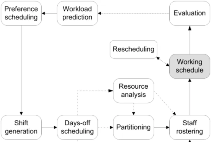
Fig. 1. The workforce scheduling process. The upper boxes represent the subphases that may occur in both mid-term and short-term planning (preprocessing phase). The subphases represented by the lower boxes (staff scheduling phase) only occur in short term planning, although information gathered from these may prove useful in future mid-term planning.
Workload prediction, also referred to as demand forecasting or demand modeling, is the process of determining the staffing levels - that is, how many
The Workforce Scheduling Process Using the
PEAST Algorithm
Nico R. M. Kyngäs, Kimmo J. Nurmi, and Jari R. Kyngäs
employees are needed for each timeslot in the planning horizon. The staffing is preceded by actual workload prediction or workload determination based on static workload constraints given by the company, depending on the situation. In preference scheduling, each employee gives a list of preferences and attempts are made to fulfill them as well as possible. The employees’ preferences are often considered in the days-off scheduling and staff rostering subphases, but may also be considered during shift generation. Together these two subphases form the preprocessing phase.
Shift generation is the process of determining the shift structure, along with the activities to be carried out in particular shifts and the competences required for different shifts. Days-off scheduling deals with the assignment of rest days between working days over a given planning horizon. Days-off scheduling also includes the assignment of vacations and special days, such as union steward duties and training sessions. Staff rostering, also referred to as shift scheduling, deals with the assignment of employees to shifts. It can also specify the starting time and duration of shifts for a given day, even though in most cases they are pre-assigned during shift generation. This subphase may include both resource analysis to examine the compatibility between the available workforce and the shifts, and partitioning in the case of massive datasets (i.e. hundreds of employees) to speed up and improve on the results of the rostering. Together these five subphases form the staff scheduling phase.
Rescheduling deals with ad hoc changes that are necessary due to sick leaves or other no-shows. The changes are usually carried out manually. Finally, participation in evaluation ranges from the individual employee through personnel managers to executives. A reporting tool should provide performance measures in such a way that the personnel managers can easily evaluate both the realized staffing levels and the employee satisfaction. When necessary, parts of the whole workforce scheduling process may be restarted. Workforce scheduling consists roughly of everything from determining the needs of the customers to determining the exact schedule of each employee.
The workforce scheduling process presented in this paper is mostly concerned with short-term planning, as defined in [10]. We have chosen to split the problem into subphases as seen in Fig. 1. This may cause problems in extremely difficult cases, due to the search space at each subphase being constrained by the choices made during previous subphases. This would be an untenable approach for finding the global optimum for most problems. However, our goal is to find a good enough solution for a broad range of problems. Our subphase-based approach is flexible enough to achieve this goal. Another benefit is decreased computational complexity due to the constantly narrowing search space.
The staff scheduling phase can be solved using computational intelligence. Computational workforce scheduling is key to increased productivity, quality of service, customer satisfaction and employee satisfaction. Other advantages include reduced planning time, reduced payroll expenses and ensured regulatory compliance.
III. THE PREPROCESSING PHASE
The preprocessing phase is the foundation upon which the actual staff scheduling phase is built. It may involve identifying both the needs of the customer(s) and the attributes (preferences, skills etc.) of the employees, and determining staffing requirements based on the former. This phase can be thought of as the transition between mid-term and short-term planning, since it touches both. This is the point in the workforce scheduling process where historical data and the schedules of previous planning horizons are most useful.
A. Workload prediction/determination
The nature of determining the amount and type of work to be done at any given time during the next planning horizon depends greatly on the nature of the job. If the workload is uncertain then some form of workload prediction is called for [8]. Some examples of this are the calls incoming to a call center or the customer influx to a hospital.
We define the service level SL(n) as the percentage of customers that need to wait for service for at most n seconds. Usually workload prediction aims to provide a certain service level (or above) for some fixed n. We simulate the randomly distributed workload based on historical data and statistical analysis, and find a suitable working employee structure (i.e. how many and what kinds of employees are needed) over time [11]. Computationally this approach is much more intensive than methods based on queuing theory. However, it has the benefit of being applicable to almost any real-world situation.
If the workload is static, no forecasting is necessary. For example, a local transport company might be under a strict contract to drive completely pre-assigned bus lines. In such a case shift generation may be necessary to combine the different bus lines into shifts, but the workload as such is static and thus calls for no forecasting.
B. Preference scheduling
Research by Kellogg and Walczak [12]indicates that it is crucial for a workforce management system to allow the employees to affect their own schedules. In general it improves employee satisfaction. This in turn reduces sick leaves and improves the efficiency of the employees, which means more profit for the employer. Hence we use an easy-to-use user interface that allows the employees to input their preferences into the workforce management system. This eases the organizational workload of the personnel manager. A measure of fairness is incorporated via limiting the number and type of different wishes that can be expressed per employee. We are looking into incorporating more rigorous fairness measures and more complex preferences to the system. In our experience our current system is satisfactory, yet there is always room for improvement.
IV. THE STAFF SCHEDULING PHASE A. Shift generation
Shift generation transforms the determined workload into shifts. This includes deciding break times when applicable. Shift generation is essential especially in cases where the workload is not static. In other cases companies often want to hold on to their own established shift building methods.
A basic shift generation problem includes a variable number of activities for each task in each timeslot. Some tasks are not time-dependent; instead, there may be a daily quota to be fulfilled. Activities may require competences. The most important optimization target is to match the shifts to the workload as accurately as possible. In our solutions we create the shifts for each day separately, each shift corresponding to a single employee’s competences and preferences. We do not minimize the number of different shifts. The choice between hard and soft constraints is given by the instances themselves. We have used the following list of constraints to successfully model and solve some real-world cases [16, 17]. The names have been prefixed in order to distinguish constraints between different subphases. Structural constraints:
(SGS1) No shift should contain timeslots with multiple types of activities (i.e. different tasks or both breaks and tasks).
(SGS2) No shift should contain gaps, i.e. timeslots with no activities.
Coverage constraints:
(SGC1) The number of employees at each timeslot over the planning horizon must be exactly as given (strict version) for each strictly time-dependent task.
(SGC2) The sum of the excesses of employees at each timeslot over the planning horizon must be minimized for each strictly time-dependent task. (SGC3) The sum of the shortages of employees at each timeslot over the planning horizon must be minimized for each strictly time-dependent task. (SGC4) The total workload for each task must be
carried out before a given timeslot. (SGC5) No working time should be wasted. Volume constraints:
(SGV1) The number of shifts, i.e. the number of employees at work, must be minimized.
(SGV2) Shifts of exactly k1timeslots in length must be maximized.
(SGV3) Shifts of less than k2 and over k3 in length must be minimized.
(SGV4) The average shift length should be as close to k4 timeslots as possible.
(SGV5) The lengths of the shifts must match the employees’ available hours.
(SGV6) The competences necessary to carry out the shifts must match the available workforce.
Placement constraints:
(SGP1) Shifts that start between timeslots k5 and k6 must be minimized.
(SGP2) Shifts that end between timeslots k7 and k8 must be minimized.
(SGP3) Each shift must contain a given number of breaks of certain lengths, depending on the length of the shift.
(SGP4) The breaks in any given shift must be evenly spaced and positioned in correct order.
(SGP5) For each task t define ct. Whenever task t appears in a shift, it must be as part of a stretch consisting only of task t and at least ct slots long.
(SGP6) Each shift should contain at most k9 switches from one task to another.
(SGP7) Each switch between tasks should occur during a break.
We now present a real-world case from a Finnish haulage company. The problem as it was presented to us, related to a cargo terminal of theirs, is as follows. The planning horizon is five days, extending from a Sunday evening to a Friday evening. Each hour a number M(d,h), where d=day and h=hour, of arrival manifests needs to be processed. The arrivals not handled immediately are queued, and the queue needs to be empty in the morning (6.30) and in the evening (20.30). The values of M for different days and hours are shown in Table I.
TABLEI MANIFEST ARRIVALS BY TIME
Mon Tue Wed Thu Fri
22-23 429 584 472 432 376
23-24 429 584 472 432 376
24-1 429 584 472 432 376
1-2 377 316 336 360 366
2-3 377 316 336 360 366
3-4 377 316 336 360 366
4-5 480 389 436 417 465
5-6 480 389 436 410 425
6-7 118 80 51 43 54
7-8 31 40 36 18 38
8-9 17 26 15 24 21
9-10 50 20 15 51 24
10-11 93 28 29 134 30
11-12 83 19 10 19 100
12-13 107 88 158 74 81
13-14 259 132 192 142 134
14-15 279 263 178 189 255
15-16 615 614 405 467 484
16-17 720 654 654 565 784
17-18 1055 908 913 1242 1002
18-19 912 969 847 842 863
19-20 429 476 728 854 423
shifts must be 4 to 6 hours long. Additionally, a part-time employee should have 3 shifts per week, and the total number of part-timers’ working hours must be at most 10% of the total working hours of all the employees.
The length of a timeslot is 30 minutes. The number of full-time employees was restricted to 69 in order to keep the workload of the part-time employees suitable. Thus we end up with 82 employees in total. The following hard constraints were used.
(SGS1): No shift should contain timeslots with multiple types of activities.
(SGS2): No shift should contain gaps.
(SGP3): Each shift must contain a 30-minute lunch break.
(SGV5): Each shift’s length must be within the allowed limits of the corresponding employee.
The following soft constraints were used.
(SGP4): For shift s, let ds be the distance of its break from the midpoint of the shift in slots (it does not matter if the optimal positions are not integers), and let as be 0.25 × (length of s). If ds > as, then a cost of round(ds –as) is incurred. (SGC4) + (SGC5):
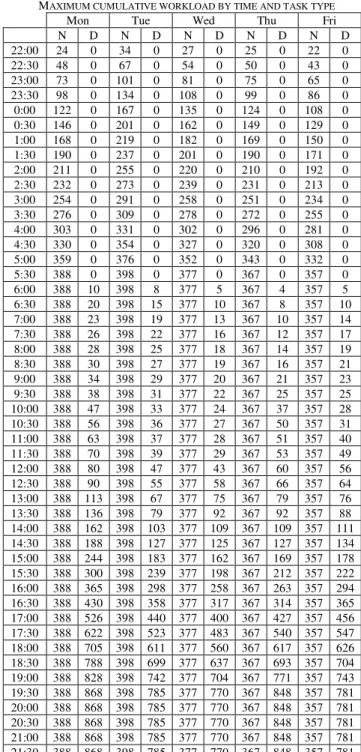
A compound constraint is used in order to make sure that the queue of arrivals is empty at 6.30 and 20.30, and that no working time is lost due to having too much workforce at work too early. The cumulative effective workload CEW[day, type, time] represents the workload that has effectively been contributed to handling the manifests up to timeslot time. Itis calculated as
where w is the number of workers scheduled to do a certain task at a certain time and MCS is the maximum cumulative workload given in Table III. For each day, the penalty given is the sum of differences between total workload and effective workload for day and night tasks.
TABLEII
COMPARISON BETWEEN OUR SOLUTION AND A MANUAL SOLUTION Our solution Manual solution
Total working minutes (actual) 175020 201300
Effective working minutes (actual) 158700 144330
Total job minutes (goal) 178170 178170
Job completion % 89 % 81 %
% of wasted working time 9 % 28 %
The results are briefly described in Table II along with comparative numbers from the company’s own solution. Our solution has no violations in SGP4, so the total penalty (649)
represents exactly the number of timeslots that the effective working time is short of the total time that the jobs require (649×30=178170-158700). The numbers from the company’s current scheduling method made us doubt whether all the assumptions were close enough to reality and if the data/model were precise enough, but based on our results a contract for the use of our optimization software was signed. We hope to get more precise data in the future in order to improve both our model and our solutions. In Section IV.C.3 we’ll roster the staff using the generated shifts.
TABLEIII
MAXIMUM CUMULATIVE WORKLOAD BY TIME AND TASK TYPE
Mon Tue Wed Thu Fri
N D N D N D N D N D
22:00 24 0 34 0 27 0 25 0 22 0 22:30 48 0 67 0 54 0 50 0 43 0 23:00 73 0 101 0 81 0 75 0 65 0 23:30 98 0 134 0 108 0 99 0 86 0 0:00 122 0 167 0 135 0 124 0 108 0 0:30 146 0 201 0 162 0 149 0 129 0 1:00 168 0 219 0 182 0 169 0 150 0 1:30 190 0 237 0 201 0 190 0 171 0 2:00 211 0 255 0 220 0 210 0 192 0 2:30 232 0 273 0 239 0 231 0 213 0 3:00 254 0 291 0 258 0 251 0 234 0 3:30 276 0 309 0 278 0 272 0 255 0 4:00 303 0 331 0 302 0 296 0 281 0 4:30 330 0 354 0 327 0 320 0 308 0 5:00 359 0 376 0 352 0 343 0 332 0 5:30 388 0 398 0 377 0 367 0 357 0 6:00 388 10 398 8 377 5 367 4 357 5 6:30 388 20 398 15 377 10 367 8 357 10 7:00 388 23 398 19 377 13 367 10 357 14 7:30 388 26 398 22 377 16 367 12 357 17 8:00 388 28 398 25 377 18 367 14 357 19 8:30 388 30 398 27 377 19 367 16 357 21 9:00 388 34 398 29 377 20 367 21 357 23 9:30 388 38 398 31 377 22 367 25 357 25 10:00 388 47 398 33 377 24 367 37 357 28 10:30 388 56 398 36 377 27 367 50 357 31 11:00 388 63 398 37 377 28 367 51 357 40 11:30 388 70 398 39 377 29 367 53 357 49 12:00 388 80 398 47 377 43 367 60 357 56 12:30 388 90 398 55 377 58 367 66 357 64 13:00 388 113 398 67 377 75 367 79 357 76 13:30 388 136 398 79 377 92 367 92 357 88 14:00 388 162 398 103 377 109 367 109 357 111 14:30 388 188 398 127 377 125 367 127 357 134 15:00 388 244 398 183 377 162 367 169 357 178 15:30 388 300 398 239 377 198 367 212 357 222 16:00 388 365 398 298 377 258 367 263 357 294 16:30 388 430 398 358 377 317 367 314 357 365 17:00 388 526 398 440 377 400 367 427 357 456 17:30 388 622 398 523 377 483 367 540 357 547 18:00 388 705 398 611 377 560 367 617 357 626 18:30 388 788 398 699 377 637 367 693 357 704 19:00 388 828 398 742 377 704 367 771 357 743 19:30 388 868 398 785 377 770 367 848 357 781 20:00 388 868 398 785 377 770 367 848 357 781 20:30 388 868 398 785 377 770 367 848 357 781 21:00 388 868 398 785 377 770 367 848 357 781 21:30 388 868 398 785 377 770 367 848 357 781
The maximum cumulative workload MCS[day, type, time] for both night (N) and day (D) tasks, calculated from M[day, time] using the
efficiency assumption of the employees based on the time of day and assuming that the workload is evenly distributed during each hour.
B. Days-off scheduling
Days-off scheduling decides the rest days and the working
CEW day type time, , =
MCS , , ,
min CEW , , -1 ,
w , , day type time
day type time
day type time
days of the employees. It is based on the result of the shift generation: for each day a set of suitable employees must be available to carry out the shifts. This is the first subphase where employees’ preferences usually have a big emphasis. The choice between hard and soft constraints is highly dependent on the problem instance. The following list of constraints is a slightly modified version of the list from [18]. The constraint names have been prefixed and renumbered in order to distinguish constraints between different phases.
Coverage requirements:
(DOC1) A minimum number of employees of particular competences must be guaranteed for each shift or each timeslot.
(DOC2) A maximum number of employees of particular competences cannot be exceeded for each shift or each timeslot.
(DOC3) A balanced number of surplus employees must be guaranteed in each working day.
Regulatory requirements:
(DOR1) The required number of working days and days-off within a timeframe must be respected. (DOR2) The required number of holidays within a
timeframe must be respected.
(DOR3) The required number of free weekends (both Saturday and Sunday free) within a timeframe must be respected.
(DOR4) Employees cannot work consecutively for more than k3 days (the maximum length of a work stretch).
(DOR5) Some employees cannot work on weekends or during specific hours of the day.
Operational requirements:
(DOO1) At least k4 working days must be assigned between two separate days-off.
(DOO2) An employee cannot be assigned to more than k5 weekend days within a timeframe.
(DOO3) An employee must be assigned to a particular shift or on-duty or off-duty on a particular day or during a particular timeslot.
Operational preferences:
(DOE1) Single days-off should be avoided. (DOE2) Single working days should be avoided.
(DOE3) The maximum length of consecutive days-off is k6.
(DOE4) A balanced assignment of single days-off and single working days must be guaranteed between the employees.
(DOE5) A balanced assignment of weekdays must be guaranteed between employees.
Personal preferences:
(DOP1) Assign or avoid assigning given employees to the same shifts.
(DOP2) Assign a requested day-on or avoid a requested day-off.
We have used these constraints to successfully model and solve some real-world days-off scheduling problems [13] and some nurse rostering problems [17].
C. Staff rostering
1) Resource analysis (optional)
To see if there will be any chance of succeeding at matching the workforce with the shifts while adhering to the given constraints, an analysis is run on the data. If we have already optimized the days-off, this subphase is not necessary but it may still be useful. In addition to helping the personnel manager see the problem with the data, it may help in convincing the management level that the current practices and processes of generating the schedules are simply untenable. We have developed a statistical tool for this.
2) Partitioning of massive data (optional)
Some real-world datasets are huge. They may consist of hundreds of employees with a corresponding number of jobs. Usually employees are trivially partitioned at some level, but that is not always the case. For example, consider a nationwide chain of service stations that sell food around the clock. Each station needs cooks, miscellaneous restaurant staff, cleaners, and so on. Let’s take a look at a cluster of 5 stations in the radius of 50 kilometers. Each station employs around 50 people. The staff from each can move freely between the stations, although every employee has one or more home bases, i.e. they prefer being stationed to particular stations. If the employees were bound to a singular preferred station, the staff of the stations could be rostered one station at a time, i.e. we would have a trivial partitioning of the employees. Since this will not produce optimal schedules, we need to roster all the 5×50 employees as a singular unit.
In the previous example it is still possible for us to consider the employees one station at a time, if the number of employees is very high, since it may be computationally infeasible to try to roster the whole set of employees at once. We use the PEAST algorithm to do such a partitioning in the general case, when there is no “obvious”, trivial partitioning to be done, as in [14].
We now present a real-world case from a Finnish bus company. The problem consists of rostering 175 bus drivers over a planning horizon of 2 weeks. The days-off are invariant. There are 6 different kinds of days-off. The hard constraints (from the list in section IV.C.3) of the problem are as follows.
(SRR1): The working time of an employee must be strictly less than his/her goal working time. The shift time of an employee must be greater than his/her goal working time.
(SRR3): The rest time of 9 hours must be respected between adjacent shifts.
which he/she cannot work certain shifts. (SRO3): The 3 most common kinds of days-off (90% of
all days-offs) must be whole, i.e. they cannot be immediately preceded by a shift that ends after midnight
(SRO4): There are in total 140 pre-assigned shifts. The soft constraints of the problem are as follows. (SRR1): The required number of working hours must be
respected. The total working hours of the employees range from 1200 minutes to 4815 minutes. The working minutes per day per employee range from 360 to 535. The difference (17888 minutes) between employees’ total working time goal (786750 minutes) and the sum of the working time of all the shifts (768862 minutes) should be evenly distributed among the shifts. There are 1643 shifts, which results in approximately 10.9 minutes per shift. Each employee should thus be SG(e)= 10.9 × (number of working days of employee e) minutes short of their personal workload goal. Define S(e) as the actual shortage for employee e. If |S(e)-SG(e)| > 0.1×SG(e), then the cost given is |S(e)-SG(e)| - 0.1×SG(e). This ensures fairness in regard to the working time. The arbitrary threshold is used, since the goal is to have highly similar but not necessarily equal shortages.
Additionally, the linkage time (i.e. time spent having lunch or waiting for another vehicle, totalling 24322 minutes in this instance) should be distributed evenly among the employees. This means approximately 14.8 minutes of linkage time per shift. Thus each employee should have LG(e) = 14.8 × (number of working days of employee e) linkage minutes. Define L(e) as the actual linkage time for employee e. If |L(e)-LG(e)| > 0.1×LG(e), then the cost given is |L(e)-LG(e)| - 0.1×LG(e). The linkage time is not nearly evenly distributed among different shift types. Almost 90% of all linkage time belongs to the 60% of shifts that start before 9 o’clock in the morning, which means that the early shifts have on average 6 times as much linkage time as the later shifts. Since some employees only want morning shifts while others only want later shifts, compromises have to be made.
(SRR3): Each employee should have at least 11 hours of rest time between two adjacent shifts. Each violation of this rule incurs a cost of 1.
(SRP2): There are 1102 working days with a shift type preference defined. Each unfulfilled wish incurs a cost of 1.
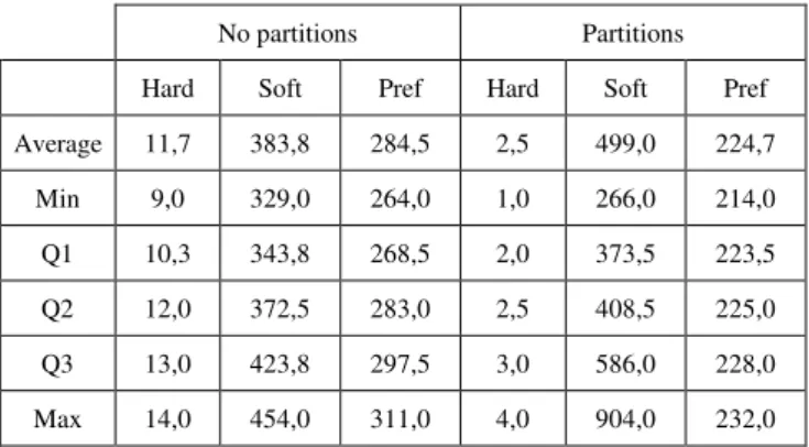
Our results both using and not using partitioning are briefly described in Table IV. One hard constraint violation is unavoidable: there is an employee whose previous
planning horizon ended with a late job, yet he has an early pre-assigned job on the first Monday of the new planning horizon, causing a rest time violation. This is a very challenging dataset and as such it shows that partitioning has its benefits. However, in order to eliminate the remaining hard constraint violations with consistency we need to either consider alternative methods or, as the preferred alternative, point out to the problem owner the inaccuracies in their current system and investigate what could be done to rectify the problems caused by their contradictory constraints.
TABLEIV
AVERAGE AND QUARTILES OF 6 RUNS FOR TOTAL HARD, TOTAL SOFT AND PREFERENCE CONSTRAINT VIOLATIONS
No partitions Partitions
Hard Soft Pref Hard Soft Pref
Average 11,7 383,8 284,5 2,5 499,0 224,7
Min 9,0 329,0 264,0 1,0 266,0 214,0
Q1 10,3 343,8 268,5 2,0 373,5 223,5
Q2 12,0 372,5 283,0 2,5 408,5 225,0
Q3 13,0 423,8 297,5 3,0 586,0 228,0
Max 14,0 454,0 311,0 4,0 904,0 232,0
3) Staff rostering (shift scheduling)
The final optimized subphase of the workforce scheduling process is staff rostering, during which the shifts are assigned to the employees. The length of the planning horizon for this subphase is usually between two and six weeks. The preferences of the employees are usually given a relatively large weight but, as before, the choice between hard and soft constraints stems from the instances themselves. The most important constraints are usually resting times and certain competences, since these are often laid down by the collective labour agreements and government regulations. Working hours of the employees are also important. We have used the following list of constraints to successfully model and solve some real-world staff rostering cases [14, 19] along with some nurse rostering cases [17].
Coverage requirements:
(SRC1) An employee cannot be assigned to overlapping shifts.
Regulatory requirements:
(SRR1) The required number of working days, working hours, shift hours and days-off within a timeframe must be respected
(SRR2) The minimum rest time within a timeframe must be respected.
(SRR3) The minimum rest time between two adjacent shifts must be respected.
(SRR5) Some employees cannot work during specific hours of the day.
(SRR6) The maximum number of shifts in a single day must be respected.
Operational requirements:
(SRO1) An employee can only be assigned to a shift he/she has competence for.
(SRO2) An employee cannot be assigned to more/less than k7 shifts of a given type within a timeframe. (SRO3) An employee assigned to a shift type t1 must not be assigned to a shift type t2 on the following day.
(SRO4) An employee must be assigned to a particular shift or on-duty or off-duty on a particular day or during a particular timeslot.
Operational preferences:
(SRE1) A balanced assignment of different shift types must be guaranteed between the employees. (SRE2) A balanced assignment of different tasks must
be guaranteed between the employees.
(SRE3) Assign or avoid a given shift type before or after a free period (days-off, vacation).
(SRE4) Assign as many wanted, and avoid as many unwanted, stints as possible.
Personal preferences:
(SRP1) Assign or avoid assigning given employees to the same shifts.
(SRP2) Assign a requested shift or avoid an unwanted shift.
(SRP3) Assign a shift (work) in a requested timeslot or assign no shift (free) to a requested timeslot.
In Section IV.A. we generated the shifts for a haulage company. Next we will schedule those shifts in order to optimize working time and resting time for each employee. In this case no separate days-off scheduling is necessary, since there are no constraints involving days-off directly.
We generated shifts for 69 full-time employees and 13 part-time employees. A full-time employee’s shifts must be 4 to 10 hours long, and the total working time over a 6-week period must be 240 hours. However, our planning horizon is only 5 days (one week), so each full-timer should have approximately 40 hours of work. A part-time employee’s shifts must be 4 to 6 hours long, and a part-time employee should have 3 shifts per week. The following hard constraints were used.
(SRR3): Each employee must have at least 7 hours of rest time between two adjacent shifts.
(SRO1): Part-timers only have competence to work shifts that are less than 6 hours in length.
The following soft constraints were used.
(SRR1): Each full-time employee should have a total working time of 2400 minutes. Each part-time employee should work 3 shifts.
(SRR3): Each employee should have at least 11 hours of rest time between two adjacent shifts. Each violation of this rule incurs a cost of 1.
We scheduled 52 full-time employees with a total working time of 2400 minutes and 17 full-time employees with a total working time of 2370 minutes, which is optimal. There are 13 violations in the rest time constraint (SRR3). Every part-timer has 3 shifts. Thus the schedule is acceptable.
V. OUR SOLUTION METHOD
The usefulness of an algorithm depends on several criteria. The two most important are the quality of the generated solutions and the algorithmic power of the algorithm (i.e. its efficiency and effectiveness). Other important criteria include flexibility, extensibility and learning capabilities. We can steadily note that our PEAST algorithm [20] realizes these criteria. The acronym PEAST stems from the methods used: Population, Ejection, Annealing, Shuffling and Tabu. Aside from workforce scheduling, it has been used to solve real-world school timetabling problems [21] and real-world sports scheduling problems [22]. We are currently investigating the impact of different components of the algorithm in order to improve it [23].We are also working on a comparison between PEAST and CPLEX performance [24].
Fig. 2. The pseudo-code of the PEAST algorithm.
Set the time limit t, no_change limit m and the population size n
Generate a random initial population of individuals Set no_change = 0 and better_found = 0
WHILE elapsed_time < t
REPEAT n times
Select an individual A by using a marriage selection with k = 3
(explore promising areas in the search space) Apply GHCM to A to get a new individual A’ Calculate the change Δ in objective function value
IF Δ < = 0 THEN Replace A with A’
IF Δ < 0 THEN
better_found = better_found + 1
no_change = 0
END IF ELSE
no_change = no_change + 1
END IF END REPEAT
IF better_found > n THEN
Replace the worst individual with the best individual Set better_found = 0
END IF
IF no_change > m THEN
(escape from the local optimum) Apply shuffling operators Set no_change = 0 END IF
(avoid staying stuck in the promising search areas too long) Update simulated annealing framework
Update the dynamic weights of the hard constraints (ADAGEN) END WHILE
The PEAST algorithm is a population-based local search method. The main difficulty for a local search is
1) to explore promising areas in the search space that is, to zoom-in to find local optimum solutions to a sufficient extent while at the same time
2) avoiding staying stuck in these areas for too long and 3) escaping from these local optima in a systematic way.
Population-based methods use a population of solutions in each iteration. The outcome of each iteration is also a population of solutions. Population-based methods are a good way to escape from local optima. The PEAST algorithm uses GHCM, the Greedy Hill-Climbing Mutation heuristic introduced in [25] as its local search method. The pseudo-code of the algorithm is given in Fig. 2.
The reproduction phase of the algorithm is, to a certain extent, based on steady-state reproduction: the new schedule replaces the old one if it has a better or equal objective function value. Furthermore, the least fit is replaced with the best one when n better schedules have been found, where n is the size of the population. Marriage selection is used to select a schedule from the population of schedules for a single GHCM operation. In the marriage selection we randomly pick a schedule, S, and then we try at most k – 1 times to randomly pick a better one. We choose the first better schedule, or, if none is found, we choose S.
The heart of the GHCM heuristic is based on similar ideas to the Lin-Kernighan procedures [26] and ejection chains [27]. The basic hill-climbing step is extended to generate a sequence of moves in one step, leading from one solution candidate to another. The GHCM heuristic moves an object, o1, from its old position in some cell, c1, to a new cell, c2, and then moves another object, o2, from cell c2 to a new cell, c3, and so on, ending up with a sequence of moves. An object is a task-based activity or a whole break (in shift generation), a day-off (in days-off scheduling) or a shift (in shift scheduling). A cell is a shift (in shift generation) or an employee (in days-off scheduling and shift scheduling). A move involves removing an object from a certain position within a cell and inserting it either into a new cell (position is invariant) or a new position (cell is invariant).
The initial cell selection is random. The cell that receives an object is selected by considering all the possible cells and selecting the one that causes the least increase in the objective function when only considering the relocation cost. Then, another object from that cell is selected by considering all the objects in that cell and picking the one for which the removal causes the biggest decrease in the objective function when only considering the removal cost. Next, a new cell for that object is selected, and so on. The sequence of moves stops if the last move causes an increase in the objective function value and if the value is larger than that of the previous non-improving move. Then, a new sequence of moves is started. The initial solution is randomly generated.
The decision whether or not to commit to a sequence of moves in the GHCM heuristic is determined by a refinement
[25] of the standard simulated annealing method [28]. Simulated annealing is useful to avoid staying stuck in the promising search areas for too long. The initial temperature T0 is calculated by
where X0 is the degree to which we want to accept an increase in the cost function (we use a value of 0.75). The exponential cooling scheme is used to decrement the temperature:
where α is usually chosen between 0.8 and 0.995. We stop the cooling at some predefined temperature. Therefore, after a certain number of iterations, m, we continued to accept an increase in the cost function with some constant probability, p. Using the initial temperature given above and the exponential cooling scheme, we can calculate the value
We choose m equal to the maximum number of iterations with no improvement to the cost function and p equal to 0.0015.
For most PEAST applications we introduce a number of shuffling operators – simple heuristics used to perturb a solution into a potentially worse solution in order to escape from local optima – that are called upon according to some rule. The most used heuristics include moving a single random object from one cell to another random cell, or swapping two random objects between two random cells. For further details on the different shuffling operators used, see [13-17, 19]. The operator is called every l/20th iteration of the algorithm, where l equals the maximum number of iterations with no improvement to the cost function.
We use the weighted-sum approach for multi-objective optimization. A traditional penalty method assigns positive weights (penalties) to the soft constraints and sums the violation scores to the hard constraint values to get a single value to be optimized. We use the ADAGEN method [25] which assigns dynamic weights to the hard constraints. The weights are updated every kth generation using the formula given in [25].
VI. CONCLUSIONS AND FUTURE WORK
We introduced the workforce scheduling process using the PEAST algorithm, along with some new datasets provided by Finnish companies. The exact datasets can be obtained from the authors by email. We believe that a great number of real-world scenarios can be modeled and solved using the framework presented in this paper. This research has contributed to improved systems for our industry partner and its customers.
We will next publish a comparison between PEAST and CPLEX performance [24]. We are also investigating the crucial components of the PEAST algorithm [23].
Our future work includes investigating the actual impact of fulfilling employees’ wishes and ensuring fairness among them in some of the companies we work with. The principal questions are, does optimization (i.e. considering preferences) actually make the employees more satisfied and
,
1
kk
T
T
.
))
log
/(
1
(
1/0
m
p
T
1 01/ log
0,
how does the company benefit from that?
Other future work includes improving and formally modeling workload prediction and resource analysis.
REFERENCES
[1] M.R. Garey and D.S. Johnson, Computers and Intractability: A Guide to the Theory of NP-Completeness. New York: Freeman, 1979.
[2] J. Tien and A. Kamiyama, “On Manpower Scheduling Algorithms,” in SIAM Rev. 24 (3), 1982, pp. 275–287.
[3] H.C. Lau, “On the Complexity of Manpower Shift Scheduling,”
Computers and Operations Research 23(1), 1996, pp. 93-102. [4] D. Marx, “Graph coloring problems and their applications in
scheduling,” Periodica PolytechnicaSer. El. Eng. 48, 2004, pp. 5–
10.
[5] L. Di Gaspero, J. Gärtner, G. Kortsarz, N. Musliu, A. Schaerf and W. Slany, “The minimum shift design problem,” Annals of Operations Research, 155(1), 2007, pp. 79–105.
[6] G.B. Dantzig, “A comment on Edie’s traffic delays at toll booths,”
Operations Research 2, 1954, pp. 339–341.
[7] H.K. Alfares, “Survey, categorization and comparison of recent tour scheduling literature,” Annals of Operations Research 127, 2004, pp.
145-175.
[8] A.T. Ernst, H. Jiang, M. Krishnamoorthy, and D. Sier, “Staff scheduling and rostering: A review of applications, methods and models,” European Journal of Operational Research 153 (1), 2004,
pp. 3-27.
[9] A. Meisels and A. Schaerf, “Modelling and solving employee timetabling problems,” Annals of Mathematics and Artificial Intelligence 39, 2003, pp. 41-59.
[10] P. De Causmaecker and G. Vanden Berghe, “Towards a reference model for timetabling and rostering,” Annals of Operations Research 194 (1), 2012, pp. 167-176.
[11] K. Nurmi, N. Kyngäs and J. Salli, “A workload prediction, staffing and shift generation method for contact centers,” in Proc. of the 4th EURO Working Group on Stochastic Modeling, Paris, France, 2012.
[12] D. L. Kellogg and S. Walczak, “Nurse Scheduling: From Academia to Implementation or Not?”, Interfaces 37 (4), 2007, pp. 355-369. [13] J. Kyngäs and K. Nurmi, “Days-off Scheduling for a Bus
Transportation Company,” International Journal of Innovative Computing and Applications3 (1), 2011, pp. 42-49.
[14] N. Kyngäs, K. Nurmi and J. Kyngäs, “Optimizing Large-Scale Staff Rostering Instances,” Lecture Notes in Engineering and Computer Science: Proceedings of The International MultiConference of Engineers and Computer Scientists, Hong Kong, 2012, pp.
1524-1531.
[15] N. Kyngäs, D. Goossens, K. Nurmi and J. Kyngäs, “Optimizing the Unlimited Shift Generation Problem,” in Proc. of the International Conference on the Applications of Evolutionary Computation,
Malaga, Spain, 2012, pp. 508-518.
[16] N. Kyngäs, K. Nurmi and J. Kyngäs, ”Solving the person-based multitask shift generation problem with breaks,” IEEE SSCI 2013, submitted for publication.
[17] N. Kyngäs, K. Nurmi, E.I. Ásgeirsson and J. Kyngäs, ”Using the PEAST Algorithm to Roster Nurses in an Intensive-Care Unit in a Finnish Hospital,” in Proc of the 9th Conference on the Practice and Theory of Automated Timetabling (PATAT), Son, Norway, 2012. [18] E.I. Ásgeirsson, J. Kyngäs, K. Nurmi and M. Stølevik, “A Framework
for Implementation-Oriented Staff Scheduling”, in Proc of the 5th Multidisciplinary Int. Scheduling Conf.: Theory and Applications (MISTA), Phoenix, USA, 2011, pp. 308-321.
[19] K. Nurmi, J. Kyngäs and G.Post , “Driver Rostering for a Finnish Transportation Company”, in Ao, Sio-Iong (ed.): IAENG Transactions on Engineering Technologies Volume 7, Springer, USA, 2012.
[20] J. Kyngäs, “Solving Challenging Real-World Scheduling Problems,” Ph.D. dissertation, Dept. of Information Technology, University of Turku, Finland, 2011. Available: http://urn.fi/URN:ISBN:978-952-12-2634-2
[21] K. Nurmi and J. Kyngäs, “A Framework for School Timetabling Problem,” Proceedings of the 3rd Multidisciplinary International Scheduling Conference: Theory and Applications, Paris, France,
2007, pp. 386–393.
[22] J. Kyngäs and K. Nurmi, “Scheduling the Finnish Major Ice Hockey League,” Proceedings of the IEEE Symposium on Computational Intelligence in Scheduling, Nashville, USA, 2009.
[23] N. Kyngäs, K. Nurmi and J. Kyngäs, “Crucial Components of the PEAST Algorithm in Solving Real-World Scheduling Problems,” 2nd International Conference on Software and Computer Applications, to be submitted for publication.
[24] N. Kyngäs, D. Goossens, K. Nurmi and J. Kyngäs, ”PEAST versus CPLEX,” Multidisciplinary International Scheduling Conference: Theory and Applications, to be submitted for publication.
[25] K. Nurmi, “Genetic Algorithms for Timetabling and Traveling Salesman Problems,” Ph.D. dissertation, Dept. of Applied Math., University of Turku, Finland, 1998. Available: http://www.bit.spt.fi/cimmo.nurmi/dissertation/cimmodis.zip [26] S. Lin and B. W. Kernighan, “An effective heuristic for the traveling
salesman problem,” Operations Research 21, 1973, pp. 498–516.
[27] F. Glover, “New ejection chain and alternating path methods for traveling salesman problems,” Computer Science and Operations Research: New Developments in Their Interfaces, edited by Sharda, Balci and Zenios, Elsevier, 1992, pp. 449–509.