Robust high-cycle fatigue stress threshold optimization under
uncertain loadings
Abstract
This paper proposes a strategy to achieve robust optimiza-tion of structures against high-cycle fatigue when a poten-tially large number of uncertain load cases are considered. The strategy is heavily based on a convexity property of some of the most commonly used high-cycle design criteria. The convexity property is rigorously proven for the Crossland fa-tigue criterion. The proof uses a perturbation technique and involves the principal stress components and analytical ex-pressions for the applicable fatigue criteria. The multiplicity of load cases is treated using load ratios which are bounded but are otherwise free to vary within certain limits. The strategy is applied to a notched plate subject to traditional normal and shear loadings that possess uncertain or unspec-ified components.
Keywords
robust optimization, fatigue, convexity
Alfredo R. de Fariaa,∗ and Roberto T. C. Frota Jr.b
Dept. of Mechanical Engineering, Instituto Tecnol´ogico de Aeron´autica
CTA - ITA - IEM, S˜ao Jos´e dos Campos, SP 12228-900, Brazil
a
tel.: 55-12-39475901;fax: 55-12-39475967
b
Tel. 55-12-39475901; fax: 55-12-39475967
Received 22 Mar 2012; In revised form 10 May 2012
∗Author email: [email protected]
1 INTRODUCTION
Traditionally, structural design does not take into account fatigue life issues. Engineers con-ceive projects based on parameters such as stress limits, maximum displacements, fundamental frequency and buckling. Nevertheless, structures break down even when admissible loads, de-termined by the design criteria above, are applied. Commonly, it occurs after a long time the structure becomes operational and the cause of failure is the end of the component fatigue life. In the aerospace industry several aircraft structural components deserve full attention from the fatigue point of view. In the fuselage upper panels, windshield, door frames, pressure domes, wing and empennage connections and engine pylon are sensitive components. In the wing lower panels, spars, landing gear fixtures, flap and aileron connections, and engine pylon are all prone to fatigue. Moreover, vertical and horizontal tails should be carefully designed for fatigue.
method with a robustness strategy.
Mrzyg l´od and Zieli´nski [9, 10], without using a robust technique, implemented a structural optimization analysis adapting the time load history in a car front suspension arm regarding eight geometric decision variables, using the Dang Van fatigue criterion as a constraint and minimizing the objective function computed by the arm mass. The optimization method applied was a probabilistic search based on evolutionary algorithms, with an optimum result of 5.6% decrease of arm mass at the 29th generation. Certainly, a large number of finite element simulations were performed to achieve this result, spending a large calculation time.
Steenackers et al. [13] integrated an optimization method with a robustness strategy ap-plied to the slat track (airplane component) finite element model taking into account the uncertainty of design parameters. They concluded that in order to obtain accurate results, an extensive computation time is necessary to run a large number of Monte Carlo simulations in combination with FE models.
Jung and Lee [5] proposed a method for robust optimization problems which conjugates the probability in design process and sensitivity analysis. Moreover they used the advanced first-order second moment method in order to reduce the calculation time. This method has the advantages of gradient-based optimization methods, since the second-order sensitivity information is not required, but the first-order sensitivity information is still necessary.
d’Ippolito et al. [3] introduce a methodology based on reliability analysis and design optimization in order to ensure robustness for their structural design considering fatigue life of its components. A probabilistic optimization method to fatigue life based on strain-life approach was implemented. The authors used a hybrid meta-model/FE strategy to save computation time. Besides a quadratic response surface model based on design of experiments (DOE) results was necessary in order to reduce the number of FE analysis.
This work presents a new robust approach in metallic structural design optimization prob-lem considering (multiaxial) high-cycle fatigue criteria. For the purpose of saving compu-tational time, removing sensitivity analysis of design variables and performing a minimum number of finite element analyses as a possible, the optimization strategy is based on extreme modeling which adds robustness to the optimal design. It is necessary to combine this tech-nique with convexity of fatigue criteria. A numerical example was solved applying the proposed robust optimization technique and the results were discussed.
2 LOADING REPRESENTATION AND PROBLEM FORMULATION
Consider an arbitrary structure with boundary conditions and L applied loadings shown in Fig. 1. A 2D sketch is drawn to facilitate visualization but 3D structures can also be resolved under the approach to be developed. The regions of application of the loadings are assumed to be fixed. This assumption rules out the class of moving loads [2] but is generally accepted in the context of fatigue investigations. Moreover, moving load problems induce relevant dynamic effects which are disregarded in high-cycle fatigue studies.
x y rL pL
σσσσ(x, t)
x
rl pl
r1 p1
Figure 1 Applied loadings
from all the loadings applied. Admitting that the loadings vary with time, the stress tensorσ
also varies with time. Additionally, since linear elasticity is assumed, the resulting stress state is the summation of the stresses produced by individual loadings:
σ=r1σ1+...+rLσL, (1)
whereσlrelates to the loading pl. The principle of superposition embedded in Eq. (1) is valid
for linear elasticity. In nonlinear problems Eq. (1) is no longer applicable. However, since the high-cycle fatigue stress thresholds are well below the yield stress, linearity is a very reasonable assumption in the present analysis.
The load ratiosr1, ...,rLrepresent the relative contribution of the loadings and are bounded
by 0≤rl ≤1 for all l =1, ..., L. Usually the loadings are not applied simultaneously and the
load ratios may obey a given relationship to reflect it. A useful relation is the linear convex combination r1+...+rL =1 which assumes that the relative contribution of the loadings add
up to 100%. A natural question that arises refers to the most dangerous loading combination. As an example, consider only two loadings: p1and p2. What combination leads to the worst
situation in terms of fatigue: (i) r1=1, r2=0, (ii) r1=0, r2=1, (iii) r1=0.5,r2=0.5 or (iv)
another combination where r1+r2=1? This question will be answered in this paper.
Any loading pl is written in terms of two components as in Eq. (2)
pl=pml +r a l(t)p
a
l (2)
where the superscripts m andawere adopted to comply with usual terminology [6] in fatigue investigations: m relates to the mean (average) of the loading component whereas areflects amplitude and time variability. Parameterral(t)varies with time and is usually harmonic (e.g. sin(ωt+φ)) in traditional fatigue investigations. pml andp
a
l are nominal or reference loadings
that may be known from the loading envelope of the structure.
When rla(t)are specified functions of time and the load ratios rl introduced in Eq. (1) are
fixed (or known) a traditional optimization procedure can be proposed considering the loading trajectory in time along with a suitable multiaxial fatigue criteria [11, 12]. On the other hand, whenever uncertainties are present in eitherrl orrla(t), more elaborate strategies are required
The optimization strategy proposed in this work to handle the lack of specification in both rl and ral(t) is based on extreme modeling. The extreme modeling adds robustness to
the optimization effectively eliminating sensitivity of optimal designs against variations in the uncertain loadings. However, in order to be economical, the extreme modeling technique should work in conjunction with convexity properties. In essence the extreme modeling technique obtains optimal designs against not only one particular load case, but against an entire space of admissible loadings.
Uncertainty is introduced in the problem admitting thatrlandral are not known beforehand
but vary within bounds for all instants of timet. These box constraints, mathematically defined in Eq. (3), guarantee a bounded problem. In practice this means that a reasonable estimative of the range of variability ofrl and ral must be available.
0≤rl≤1, ∑Ll
=1rl=1, (r a
l)MIN≤ral ≤(ral)MAX. (3)
Notice that Eq. (3) does not assume beforehand how the load ratios may vary with time. This is an important aspect of the loading representation since nonharmonic and asynchronous loadings can be considered. Therefore, time variability of ral(t) becomes unimportant since what essentially matters are the side constraints(ral)MIN and(ral)MAX. Statistically the
inter-pretation for time independence is thatrla is assumed to have uniform probability of attaining any value contained within the box defined in Eq. (3c).
The traditional optimization problem may be posed as volume minimization under the constraint that a given multiaxial fatigue criterion is satisfied, e.g. Dang Van [14], Crossland [1], McDiarmid [7], Findley [4], Mamiya [6], among others:
min
θ V(
θ)
s.t.∶ max
x
max
r
σc(θ,x,r)≤b (4)
where θ is the vector of design variables such as thickness distribution over a plate or cross
section dimensions of stiffeners in a reinforced panel, V(θ) is the total structural volume, σc
is the critical fatigue stress which depends on the stress tensor σ atx, b is the fatigue stress
threshold, andr(t)={ r1 r1a(t) r2 r2a(t) r3 r3a(t) ... rL rLa(t) }
T. Notice that ris a
function of time and so isσc.
Equation (4) shows that the most demanding procedure in the solution of the optimization problem is the computation of the constraints which involves double maximization of σc over
xand r(t). Additionally, the constraint in Eq. (4) is nondifferentiable with respect to θ since
the worst r certainly varies with θ. The next section shows how to significantly simplify the
double maximization problem required to evaluate the constraints present in Eq. (4).
3 CONVEXITY OF FATIGUE CRITERIA
The critical fatigue stress σc is calculated based on the stress tensor σ at a particular point
maximization problem is twofold. Firstly, consider a fixed pointx1and vary r. Once the most
dangerous load ratios r1 are obtained for point x1 another point x2 is to be assessed and its
most dangerous load ratios r2 obtained. Observe that, since time independence is assumed,
usuallyr1≠r2.
Computation of the worstris an important part of the constraint evaluation which can be sped up if σc is more carefully examined. Since most multiaxial stress fatigue criteria depend
on the principal stresses of σ it is worth investigating how the principal stresses vary as σ
is perturbed. Assume that vector r produces a given stress tensor at point x which can be computed as in
σ=
L ∑ l=1
rlσl= L ∑ l=1
rl[σml +r a l(t)σ
a l]=
L ∑ l=1
[rlσml +rl(t)σal], (5)
where σm
l and σ
a
l relate, respectively, to the loadings p m
l and p
a
l defined in Eq. (2). The
newly defined parameterrl(t)is simply the productrl×rla(t)and, according to Eqs. (3a) and
(3c), obey the relationship
0≤rl(t)≤(rla)MAX. (6)
Equation (5) is linear in r1, r1, ..., rL, rL. Therefore, a first order perturbation in these
parameters lead to a first order perturbation in σ of the type σ+δσ, not containing higher
order terms δ2σ,δ3σ, etc.
The principal stresses are computed from the eigenvalue problem stated in Eq. (7)
(σ−λI)n=0, (7)
where I is the identity tensor, λ is the principal stress and n is the principal direction. The perturbed eigenvalue problem is
[(σ+δσ)−(λ+δλ+δ2λ+...)I](n+δn+δ2n+...)=0. (8)
Equation (8) can be split into higher order problems such that the first order problem is
(δσ−δλI)n+(σ−λI)δn=0 (9)
and the second order problem is
−(δ2λ)n+(δσ−δλI)δn+(σ−λI)δ2n=0. (10)
Premultiplication of Eq. (9) by nT, use of Eq. (7), symmetry of σ and the fact that
nTn=1 yields
Equation (11) shows how the principal stresses vary when r is perturbed. However, not much useful information can be retrieved from it. Premultiplication of Eq. (10) by nT, use of Eqs. (7) and (9), and the fact thatnTn=1 yields
δ2λ=−δnT(σ−λI)δn. (12)
Equation (12) gives important information regarding the sign of the second derivative ofλ
(the principal stresses). Notice thatσ can be written asσ=NΛNT whereNis the matrix of
eigenvectors (stored columnwise) andΛ is the diagonal matrix whose trace is composed of the principal stresses σI,σII, σIII with σI ≥σII ≥σIII. It is clear that NTN=NNT =I holds.
Hence, Eq. (12) can be rewritten as
δ2λ=−δnTN ⎡⎢ ⎢⎢ ⎢⎢ ⎣
σI−λ 0 0
0 σII−λ 0 0 0 σIII−λ
⎤⎥ ⎥⎥ ⎥⎥ ⎦
NTδn. (13)
There are two important situations: (i)λ=σI and (ii) λ=σIII. Whenλ=σI the diagonal
matrix in Eq. (13) is negative semi-definite and when λ=σIII it is positive semi-definite. In
one case δ2λ=δ2σI≥0 and in the otherδ2λ=δ2σIII ≤0.
The conclusions just drawn can be immediately employed to prove convexity with respect to r1, r1, ..., rL, rL of one of the most commonly used high-cycle fatigue criterion in finite
element analyses: Crossland [1].
The Crossland (σCR) stresses can be expressed as
σCR=
√
J2+κCRσH, (14)
where κCR is a parameter that can be expressed from data of two fatigue tests (reversed
bending and reversed torsion), σH =(σI+σII+σIII)/3 is the hydrostatic stress (three times
the trace of the stress tensor) andJ2is the second invariant of the stress deviator tensor given
by
J2=
1 6
√
(σI−σII)2+(σI−σIII)2+(σII−σIII)2. (15)
The square root of J2 appearing in Eq. (14) is an amplitude and not an instantaneous
value. The calculation of this amplitude necessitates the definition of a complete load cycle. From a complete load cycle one can calculate the amplitude of the square root of J2 and the
maximum hydrostatic stress σH occurring within this cycle to apply the Crossland criterion.
Notice, however, that time dependancy is not an issue anymore since extreme modeling is being applied (see Eqs. (3a) and (6)). Since trace (3σH) is a linear function of σI ,σII ,σIII
its second variation (or derivative) is zero, i.e., δ2σH =0. On the other hand,J2 is a quadratic
function of σI ,σII , σIII meaning that its second variation must be nonnegative, what also
implies that the second variation of √J2 is also nonnegative, i.e.,δ 2√
J2≥0. It follows that
δ2σCR=δ
2√
J2+κCRδ
2
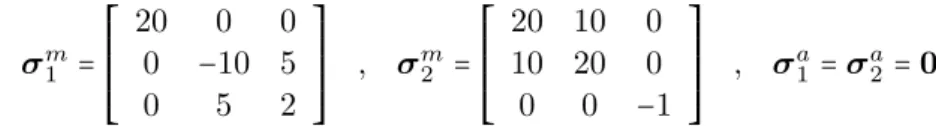
As an example, consider two reference stress states given by
σm1 = ⎡⎢ ⎢⎢ ⎢⎢ ⎣
20 0 0 0 −10 5 0 5 2
⎤⎥ ⎥⎥ ⎥⎥ ⎦
, σm2 = ⎡⎢ ⎢⎢ ⎢⎢ ⎣
20 10 0 10 20 0 0 0 −1
⎤⎥ ⎥⎥ ⎥⎥ ⎦
, σa1=σa2=0
and assume two load ratios r1=r and r2=1−r, 0≤r ≤1, are associated with σm1 and σ
m
2,
respectively, such that the resulting stress state is σ = r1σm1 +r2σm2. Taking κCR = 0.5 it
is possible to draw the stress curves shown in Fig. 2. As expected, it is clear that σCR is a
convex function ofr. Moreover, notice that trace is a linear function orr, what is also expected sinceδ2σH =0. Nothing can be stated about the convexity of the second principal stress σII.
Actually, it is seen that the sign ofδ2σII is either positive or negative.
r
σ
0.00 0.25 0.50 0.75 1.00
-15 -10 -5 0 5 10 15 20 25 30 35 40
σI
σII
σIII
σH
σCR
Figure 2 Stress curves for varying load ratios
4 ROBUST OPTIMIZATION STRATEGY
Equation (4) states the robust optimization problem that must be solved in order to find the optimal design θ. In the previous section it was proven that the critical fatigue stress σc is
convex with respect to variations in the applied loadings r, i.e., δ2σc ≥ 0, at least for the
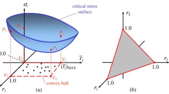
Convexity of σc with respect to variations in the load ratios can be schematically seen in
Fig. 3a. The critical stress surface is constructed by computing σc for different load ratios
represented generically by ri and rj. It must be clear that only two axes of load ratios are
drawn to permit visualization in 3D. However, many more may be present as explained in section 2. The load ratios are represented by dots in the rirj plane. Notice that the loading
envelope described in Eqs. (3a) and (6) is highlighted in Fig. 3a and termed convex hull. This terminology is justified by the fact that any other set of load ratios, represented by dots within the convex hull, can be written as a linear convex combination of the verticesV1−V4 of
the convex hull. Figure 3b shows the geometrical representation of Eq. (3b) where the plane
r1+r2+...+rL=1 can be seen.
With regard to the optimization strategy, constraint evaluation in Eq. (4) requires solution of the inner loop that maximizes σc with respect to r. This inner maximization problem can
be solved by checking the projectionsP1−P4of the convex hull verticesV1−V4onto the critical
stress surface. The worst possible load ratios is the one whose pointPk is associated with the
greatest σc. Notice that, in a situation where there are several loadings applied, even using
the convexity ofσcentails computation of a very large number of possibilities. For a structure
withL loadings the number of possibilities isL×2L, whereLcomes from the vertices defined
by Eq. (3b) and 2L comes from the box constraints defined in Eq. (6). Since linearity of the
mechanical response is assumed, 2L load cases can be computed beforehand and the result stored for evaluation of the worstσc, beingLloadingspml andLloadingsp
a
l. The next section
presents an example to clarify this point.
ri
σc critical stress
surface
convex hull
rj (rj)MAX
0.0
1.0
V1 V2
V3
V4 P2
P4 P1
ri
rj
rk
1.0
1.0 1.0
(a) (b)
P3
Figure 3 Convexity of critical fatigue stress
5 NUMERICAL EXAMPLE
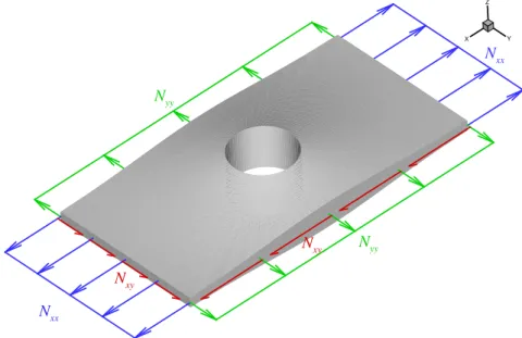
The rectangular notched plate shown in Fig. 4 is used as an example. It has length 1.0 m, width 0.5 m and circular notch with radius 0.1 m located at the plate center. Notice that the plate has a nonuniform thickness distribution and the loadings may have mean and amplitude components as expressed by Eq. (2).
X Y
Z
Nxy
Nxx
Nxx
Nyy Nyy
Nxy
Figure 4 Notched plate with loadings with nonuniform thickness distribution
A finite element code was developed to obtain the critical fatigue stress σc based on the
Crossland criterion. This code employs the 4-noded quadrilateral element with the usual bilinear shape functions
N1(ξ, η)=
1
4(1−ξ)(1−η) N2(ξ, η)= 1
4(1+ξ)(1−η)
N3(ξ, η)=
1
4(1+ξ)(1+η) N4(ξ, η)= 1
4(1−ξ)(1+η). (17)
The element stiffness matrix Ke can be computed by
Ke=∫
Ωeh(x, y)B
TCBdΩ, (18)
where
B= ⎡⎢ ⎢⎢ ⎢⎢ ⎣
Φ,x 0
0 Φ,y
Φ,y Φ,x
⎤⎥ ⎥⎥ ⎥⎥ ⎦
C−1
= ⎡⎢ ⎢⎢ ⎢⎢ ⎣
1/E −ν/E 0 −ν/E 1/E 0 0 0 1/G
⎤⎥ ⎥⎥ ⎥⎥ ⎦
(19)
and the displacements u and v can be interpolated using the respective nodal values u1, u2,
u3,u4 and v1,v2,v3,v4 as
u=Φ{ u1 u2 u3 u4 }T v=Φ{ v1 v2 v3 v4 }T. (20)
Notice that the integral in Eq. (18) involves the thicknessh(x, y)which varies over the ele-ment domain. The thickness distribution of the plate is assumed to be adequately represented by nodal thicknesses such that, similarly to Eq. (20), it can be interpolated as
h=Φ{ h1 h2 h3 h4 }T (21)
and integration in Eq. (18) is numerically carried out using 2× 2 Gaussian quadrature. The mesh shown in Fig. 5 with bilinear elements was used to model the plate. Refinement around the notch boundary was ensured because this is the region where stress concentrations shall occur.
Figure 5 Meshed notched plate
The optimization strategy selected to solve Eq. (4) is topometric, i.e., plate volume mini-mization is achieved through thickness variation. The procedure implemented is simple:
i. For a given thickness distributionθi find the worstσc at all nodes
ii. For each nodeI, update thickness hI,i+1=hI,i∗σcI/b
Figure 6 presents the flowchart of the optimization procedure described here and in the previous section. The stresses evaluated at the nodal positions are computed on average, i.e., if two or more elements share node I, then the stress is given by the average of the stresses computed using interpolation functions and nodal displacements of these two or more elements.
select initial thickness distribution
i = i + 1
solve L × 2L linear problems
compute worst σcI for every node I in the mesh
update thickness distribution
hI,i+1 = hI,i × σcI / b i = 0
for all nodes
hI,i+1 = hI,i ?
end
NO
YES
Figure 6 Optimization flowchart
The three loadings (L=3) to be applied in this plate example are those illustrated in Fig.
4. They are more precisely described in Tab. 1, split into mean and average components, and amplitude parameters. According to Tab. 1 the loadings are limited to 0≤Nxx ≤800 kN/m,
0≤Nyy≤200 kN/m, −400 kN/m≤Nxy≤+400 kN/m and, in theory,L×2L=24 vertices must
be assessed.
Table 1 Definition of loadings and load ratios
Load pm (kN/m) pa (kN/m) (ra)MIN (ra)MAX
Nxx Nxxm =400 N
a
xx=400 -1.0 1.0
Nyy Nyym=100 N
a
yy=100 -1.0 1.0
Nxy Nxym=0 N
a
xy =400 -1.0 1.0
Tables 2-4 give clear account about how this conclusion is drawn. Consider for instance Tab. 2 wherer1=1 andr2=r3=0. r1relates to the normal loadNxx,r2relates to the normal load
Nyy and r3 relates to the shear loadNxy. The first three columns of Tab. 2 correspond to all
possible permutations ofra
1,r2aandr3awhich can assume only two values (-1 or +1) according to
Tab. 1. Columns 4-6 of Tab. 2 are the values ofr1,r2andr3computed by the productrl=rlral
(see Eq. (5)). Finally, columns 7-9 of Tab. 2 are computed using Tab. 1 and Eq. (5). For example, the fifth row is obtained computingNxx=r1Nxxm+r1Nxxa =1×400+1×400=800 kN/m,
Nyy=r2Nyym+r2Nyya =0×100+0×100=0 kN/m andNxy =r3Nxym+r3Nxya =0×0+0×400=
0 kN/m.
Examining Tabs. 2-4 it can be concluded that most of the loading vertices correspond to null loadings such that only four of them must be evaluated: (i) Nxx =800 kN/m, Nyy =
0 kN/m,Nxy=0 kN/m, (ii)Nxx=0 kN/m,Nyy=200 kN/m,Nxy =0 kN/m, (iii)Nxx=0 kN/m, Nyy =0 kN/m, Nxy =400 kN/m, (iv) Nxx =0 kN/m, Nyy =0 kN/m, Nxy =−400 kN/m. This
simplification is not always as straightforward since the existence of nonzero loading vertices and complex geometries of structural components commonly lead to situations where obvious undangerous loadings cannot be discarded beforehand.
Table 2 Determination of loading vertices forr1=1,r2=r3=0
ra1 ra2 r3a r1 r2 r3 Nxx (kN/m) Nyy (kN/m) Nxy (kN/m)
-1 -1 -1 -1 0 0 0 0 0
-1 -1 1 -1 0 0 0 0 0
-1 1 -1 -1 0 0 0 0 0
-1 1 1 -1 0 0 0 0 0
1 -1 -1 1 0 0 800 0 0
1 -1 1 1 0 0 800 0 0
1 1 -1 1 0 0 800 0 0
1 1 1 1 0 0 800 0 0
Table 3 Determination of loading vertices forr2=1,r1=r3=0
ra1 ra2 r3a r1 r2 r3 Nxx (kN/m) Nyy (kN/m) Nxy (kN/m)
-1 -1 -1 0 -1 0 0 0 0
-1 -1 1 0 -1 0 0 0 0
-1 1 -1 0 1 0 0 200 0
-1 1 1 0 1 0 0 200 0
1 -1 -1 0 -1 0 0 0 0
1 -1 1 0 -1 0 0 0 0
1 1 -1 0 1 0 0 200 0
Table 4 Determination of loading vertices forr3=1,r1=r2=0 ra1 r
a
2 r
a
3 r1 r2 r3 Nxx (kN/m) Nyy (kN/m) Nxy (kN/m)
-1 -1 -1 0 0 -1 0 0 -400
-1 -1 1 0 0 1 0 0 400
-1 1 -1 0 0 -1 0 0 -400
-1 1 1 0 0 1 0 0 400
1 -1 -1 0 0 -1 0 0 -400
1 -1 1 0 0 1 0 0 400
1 1 -1 0 0 -1 0 0 -400
1 1 1 0 0 1 0 0 400
In order to illustrate the weaknesses of the conventional optimization against single loadings five optimization cases are considered as presented in Tab. 5. Cases I-IV correspond to single loads whereas case V corresponds to the robust optimization case. The ‘±’ in case V indicates that either positive or negative shear may be applied as just discussed. It must be clear that, as implied by Eq. (5), loadings in case V are not applied simultaneously; it is actually a varying load case where the four load cases I-IV of Tab. 5 are applied as a convex combination
σ=∑4l
=1rlσl, with ∑ 4
l=1rl=1 and 0≤rl≤1.
As explained in section 4 the loading ratiosr1,r1, ...,rL,rLare free to vary but must satisfy
Eqs. (3) and (6). For optimization purposes, it was shown in section 4 that it is sufficient to check the vertices of the loading space corresponding to Nxx =800 kN/m, Nyy =200 kN/m, Nxy =+400 kN/m and Nxy=−400 kN/m, one at a time. However, the optimal design thereby obtained is guaranteed to sustain any linear convex combination of these four loadings.
Table 5 Effective loadings for optimization
Case Nxx (kN/m) Nyy (kN/m) Nxy (kN/m)
I 800 0.0 0.0
II 0.0 200 0.0
III 0.0 0.0 -400
IV 0.0 0.0 +400
V 800 200 ±400
The material properties used in the numerical example are: E = 205 GPa, ν = 0.3, κ
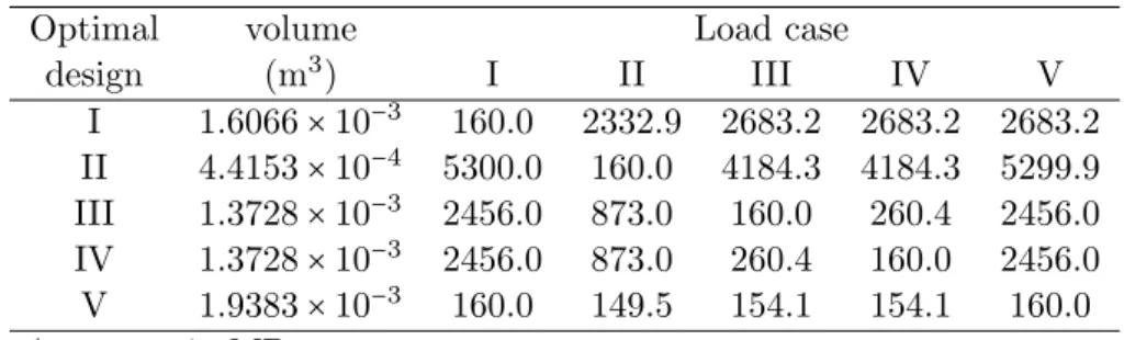
= 0.35, b = 160 MPa. Table 6 presents the volume of the optimal designs obtained and the critical fatigue stresses calculated at the loading vertices. The highest volume is associated with optimal design V since this is the robust design, i.e., the only one that can equally well sustain all load cases (σc ≤ 160 MPa). The vulnerability of the traditional optimal designs,
last column of Tab. 6 is simply the maximum value of the critical fatigue stresses.
Table 6 Critical fatigue stress for optimal designs∗
Optimal volume Load case
design (m3) I II III IV V
I 1.6066×10⁻³ 160.0 2332.9 2683.2 2683.2 2683.2 II 4.4153×10⁻⁴ 5300.0 160.0 4184.3 4184.3 5299.9 III 1.3728×10⁻³ 2456.0 873.0 160.0 260.4 2456.0 IV 1.3728×10⁻³ 2456.0 873.0 260.4 160.0 2456.0 V 1.9383×10⁻³ 160.0 149.5 154.1 154.1 160.0 ∗
stresses in MPa
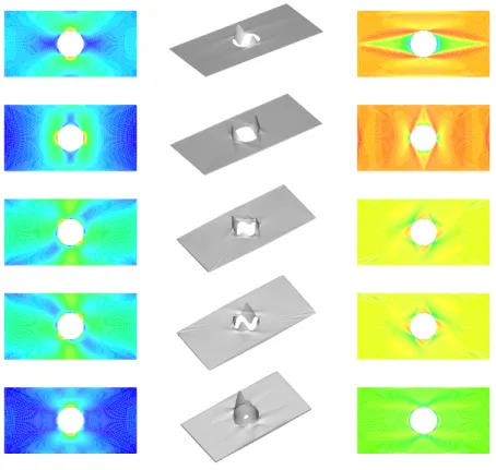
A visualization of the optimization procedure is shown in Fig. 7. Figures without scales are drawn since the intention is to give a qualitative view of the stress and thickness distributions. Rows 1 to 5 correspond to the five effective loadings described in Tab. 5. In the first column are the critical fatigue stress results for the uniform plate. In the second column are the thickness distributions of the optimal designs. In the third and last column are the the critical fatigue stress results for the optimal plates. All optimization processes began with a uniform plate 1.0 mm thick, which corresponds to an initial volume of 4.6858×10⁻⁴ m3. As shown in Fig. 7 (first column) stress concentrations occur around the notch. Therefore, although the initial structural volume is small (4.6858×10⁻⁴
m3
) compared to those obtained in Tab. 6, the initial uniform plate suffers from fatigue under all loadings.
It is clear that stress concentration regions around the notch are observed in all cases of uniform thickness distribution (red regions), whereas stresses are much more spread in the optimal designs (last column in Fig. 7). Cases III and IV are equivalent since they corre-spond simply to a change in sign of the shear loads. The thickness distribution of the robust optimal design (last row) is such that it reinforces the region around the notch where stress concentrations seen in the first column arise. Figure 7 shows optimal designs with unusual shapes (second column). It is obvious that the stress is concentrated around the notch (with a maximum value of 3 times the applied stress in single tension) and increasing the thickness can decrease this maximum value but, the question whether these shapes are acceptable is dependant on the application. In practice, some kind of smoothing may be necessary prior to actual production of optimal designs, similarly to what is observed in topology optimization.
The critical stress surface can be visualized for the plate example simulated. Figure 3b schematically shows the reference plane r1+r2+r3+r4 =1. Since in the plate example load
cases III and IV are exactly the same, except for a change in sign of the shear load, r3 and
r4 can be collapsed intor ∗
3, where positive values of r ∗
3 relate to r3 and negative values of r ∗ 3
relate tor4. Figure 8 depicts the critical stress surface where now the reference plane equation
is given byr1+r2+∣r3∗∣=1. The concavity of the surface can be clearly observed. The legend
shows values for the normalized maximum critical fatigue stress σ∗
Figure 7 Optimal design results
for the robust optimal design, 0<σ∗≤1. The highest values ofσ∗happen in the region around
the edges of the reference plane.
For the sake of comparison against Fig. 8, Fig. 9 depicts the critical stress surface obtained for the optimal design under load case I solely. Though still concave, the critical stress surface is now severely distorted. The normalized maximum critical fatigue stress σ∗
assumes now values of up to 15.7 which is way beyond the fatigue thresholdb.
6 CONCLUSIONS
σ*
0.934 0.869 0.803 0.738 0.672 0.607 0.541 0.475 0.410 0.344 0.279 0.213 0.148 0.082 0.016
r1
r2 r3*
Figure 8 Maximum critical stress surface for robust optimal design
σ*
15.671 14.571 13.471 12.372 11.272 10.172 9.073 7.973 6.873 5.773 4.674 3.574 2.474 1.375 0.275 r1 r2
r3*
The optimal results are robust against fatigue. However, from a practical view point, that is, if one must design a real structure, even the robust optimal design would hardly be manufactured. As a suggestion to obtain a viable optimal design which can be used in practice, geometric constraints could be included on the volume minimization. The simplest possibility is to consider that the plate is composed of a base plate whose thickness is uniform and fixed and external layers of variable thickness exist. A more elaborate proposal is to add constraints on the maximum thickness gradient such that the maximum difference in thickness between adjacent elements must not exceed a certain amount.
The topometric numerical optimization adopted may not result in strictly optimal designs in the global sense. However, it is a fast procedure that does not require evaluation of gradients. Notice that, although gradient of volume is easily computed, the maxxmaxrσc in Eq. (4) is a
nondifferentiable constraint. Hence, the use of gradient-based optimization procedures would require considerable effort and ingenuity to overcome the lack of necessary smoothness in the constraint.
AcknowledgmentsThis work was partially financed by the Brazilian agency CNPq (grant no. 300236/2009-3).
References
[1] B. Crossland. Effect of large hydrostatic pressures on the torsional fatigue strength of an alloy steel. InProceeding
of the International Conference on Fatigue of Metals, London & New York, 1956.
[2] A.R. de Faria. Finite element analysis of the dynamic response of cylindrical panels under traversing loads.European
Journal of Mechanics/A Solids, 23:677–687, 2004.
[3] R. dIppolito, M. Hack, S. Donders, L. Hermans, N. Tzannetakis, and D. Vandepitte. Improving the fatigue life of a
vehicle knuckle with a reliability-based design optimization approach. Journal of Statistical Planning and Inference,
139:1619–1632, 2009.
[4] W.N. Findley. Fatigue of metals under combinations of stresses. Transactions of ASME, 79:1337–1348, 1957.
[5] D.H. Jung and B.C. Lee. Development of a simple and efficient method for robust optimization. International
Journal for Numerical Methods in Engineering, 53:2201–2215, 2002.
[6] E.N. Mamiya, J.A. Ara´ujo, and F.C. Castro. Prismatic hull: a new measure of shear stress amplitude in multiaxial
high cycle fatigue. International Journal of Fatigue, 31:1144–1153, 2009.
[7] D.L. McDiarmid. A shear stress based critical-plane criterion of multiaxial fatigue failure for design and life prediction. Fatigue & Fracture of Engineering Materials & Structures, 17:1475–1484, 1994.
[8] M. McDonald and M. Heller. Robust shape optimization of notches for fatigue-life extension. Structural and
Multi-disciplinary Optimization, 28:5568, 2004.
[9] M. Mrzyg´od and A.P. Zieli´nski. Numerical implementation of multiaxial high-cycle fatigue criterion to structural
optimization. Journal of Theoretical and Applied Mechanics, 44:691–712, 2006.
[10] M. Mrzyg´od and A.P. Zieli´nski. Mutiaxial high-cycle fatigue constraints in structural optimization. International
Journal of Fatigue, 29:1920–1926, 2007.
[11] I.V. Papadopoulos, P. Davoli, C. Gorla, M. Filippini, and A. Benasconi. A comparative study of multiaxial high-cycle
fatigue criteria for metals.International Journal of Fatigue, 19:219–235, 1997.
[12] J. Papuga. Mapping of fatigue damages - program shell of FE-calculation. PhD thesis, Faculty of Mechanical
Engineering, Czech Technical University, Prague, 2005.
[13] G. Steenackers, P. Guillaume, and S. Vanlanduit. Robust optimization of an airplane component taking into account
the uncertainty of the design parameters.Quality and Reliability Engineering International, 25:255–282, 2009.