Bernardo Fitas Sarmento
Bachelor of Science in Materials Engineering
Simulation of sunlight driven CO
2
conversion to
CH
4
to satisfy a single-house
heating requirements
Dissertation submitted in partial fulfillment of the requirements for the degree of
Master of Science in Materials Engineering
Supervisor: Dr. Ana Reis Machado, Auxiliar Researcher, NOVA University of Lisbon
Co-supervisors: Dr. Manuel J. Mendes, Post-Doc Fellow and
Invited Assistant Professor, NOVA University of Lisbon
Dr. Jorge Manuel Facão, Researcher, Laboratório Nacional de Energia e Geologia
Examination Committee
Chairperson: Dr. João Paulo Borges, NOVA University of Lisbon
Simulation of sunlight driven CO2conversion to CH4to satisfy a single-house heating requirements
Copyright © Bernardo Fitas Sarmento, Faculty of Sciences and Technology, NOVA Uni-versity Lisbon.
The Faculty of Sciences and Technology and the NOVA University Lisbon have the right, perpetual and without geographical boundaries, to file and publish this dissertation through printed copies reproduced on paper or on digital form, or by any other means known or that may be invented, and to disseminate through scientific repositories and admit its copying and distribution for non-commercial, educational or research purposes, as long as credit is given to the author and editor.
This document was created using the (pdf)LATEX processor, based in the “novathesis” template[1], developed at the Dep. Informática of FCT-NOVA [2].
Ac k n o w l e d g e m e n t s
Quero começar por agradecer ao Professor Doutor Rodrigo Martins como presidente do Departamento de Ciências dos Materiais e à Professora Doutora Elvira Fortunato como directora do Centro de Investigação de Materiais por todo o apoio e dedicação em tornar o DCM e o CENIMAT em centros de ensino e de investigação de topo e por proporcionarem aos alunos as mais altas condições de ensino.
Obrigado aos meus orientadores, Profª. Doutora Ana Machado, Prof. Doutor Manuel Mendes e Doutor Jorge Facão pela oportunidade de poder participar num projecto tão interessante para a sociedade e por toda a ajuda, paciência e apoio dado no decorrer do meu trabalho.
Quero agradecer também ao DCM e a todos os professores que me abilitaram com as ferramentas necessárias que me tornaram num engenheiro e numa melhor pessoa e que continuem com o excelente trabalho de formar futuros Engenheiros de Materiais.
Um muito obrigado às pessoas que me acompanharam durante estes 5 anos, pelas horas de estudo em conjunto, pelas noitadas a fazer trabalhos por chamada, pelas brin-cadeiras, pelos sorrisos, pelas idas ao sushi, por estarem sempre lá e pelas amizades criadas para a vida toda.
Finalmente um agradecimento à minha família e muito especial à minha Mãe, Pai e Irmão, obrigado por me darem a educação e a possibilidade de frequentar a faculdade e por todo o apoio e amor incondicional.
If we are to live, We must take risks. Else our lives become Deaths in all but name. There is no struggle too vast, No odds too overwhelming, For should we fail should we fall -We will know That we have Lived.
A b s t r a c t
The rise of Earth’s atmospheric CO2 levels, primarily due to combustion of fossil fuels, has affected its ecosystems. A way to combat this is by mimicking the plants photo-synthesis by capturing CO2from the atmosphere and convert it to usable hydrocarbon
fuels, such as methane (CH4), because of the easy adaptability to the well-established infrastructure for natural gas (NG) storage, distribution and consumption. The denomi-nated “solar methane”, very similar to NG, can be produced by converting solar energy from photovoltaic (PV) panels into electricity to power a 1-step reaction on electrochemi-cal flow cell(s), using CO2and water as the feedstock. Here, we simulate solar methane
production and storage and apply it to address the energetic needs of concept build-ings that have space and domestic hot water heating requirements. A combination of solar thermal collectors (STCs) and PV panels is optimized for buildings in different Eu-ropean locations, in which the heating needs that cannot be fulfilled by the STCs are satisfied by the combustion of methane synthesized by the PV-powered electrolyzers. Var-ious combinations of situations for a whole year were studied and it was found that this auxiliary system can produce, per m2of PV area, in the worst case scenario 23.6 g/day (0.328 kWh/day) of methane in Stockholm and in the best case scenario 47.4 g/day (0.658 kWh/day) in Lisbon.
R e s u m o
O aumento dos níveis de CO2na atmosfera terrestre, principalmente devido à combustão
de combustíveis fósseis, tem afectado os ecossistemas. Uma maneira de combater isto é imitando o processo de fotossíntese das plantas ao capturar CO2da atmosfera e
conver-ter em combustíveis hidrocarbonetos utilizáveis, tal como o Metano (CH4), devido à fácil
adaptabilidade à infraestructura já estabelecida de gás natural (NG) para armazenamento, distribuição e consumo. O denominado "metano solar", muito idêntico ao NG, pode ser produzido convertendo energia solar de painéis fotovoltaicos (PV) em eletricidade para promover numa célula electroquímica a conversão de CO2 e água em metano num só passo. Neste trabalho, simulamos a produção de metano solar e o seu armazenamento para satisfazer as necessidades energéticas de edifícios de conceito com requerimentos de aquecimento ambiente e de preparação de água quente sanitária. Uma combinação de colectores solares térmicos (STC) e paineis PV são otimizados para edifícios em di-ferentes cidades Europeias. Caso as necessidades energéticas não possam ser satisfeitas pelos STCs, são satisfeitas pela combustão do metano sintetizado. Várias combinações de situações para um ano inteiro foram estudadas e descobriu-se que este sistema auxiliar pode produzir, por m2de PV area, no pior cenário 23.6 g/dia (0.328 kWh/dia) de metano em Estocolmo e no melhor cenário 47.4 g/dia (0.658 kWh/dia) em Lisboa.
C o n t e n t s
List of Figures xv
List of Tables xvii
Listings xix
Glossary xxi
Acronyms xxiii
1 Objectives and Motivation 1
2 Introduction 3
2.1 Solar Fuels Generation . . . 3
2.1.1 Integrated Photovoltaic-Electrochemical CO2Reduction . . . 5
2.2 Building Heating Requirements . . . 5
3 Architecture of the System 9 3.1 Software used . . . 9
3.1.1 TRNSYS . . . 9
3.1.2 MATLAB . . . 10
3.2 Methodology . . . 10
4 Discussion and results 11 4.1 TRNSYS Parameters . . . 11
4.1.1 Main Project . . . 11
4.1.2 Photovoltaic project . . . 18
4.2 Matlab System . . . 19
4.2.1 PV-IV script . . . 19
4.2.2 Methane production script . . . 20
4.3 Results . . . 22
4.3.1 Influence of electrodes deactivation . . . 23
4.3.2 Influence of different space heating consumption . . . . 23
4.3.3 Influence of different building location . . . . 26
4.3.4 Influence of different solar thermal collector area . . . . 27
5 Conclusion and future perspectives 31
References 33
CO N T E N T S
B Appendix: Supplementary results 41
I Annex 1 - Code used in MATLAB 55
I.1 Setup Script . . . 55
I.2 Function to Calculate IV curve . . . 60
I.3 Extrapolate function . . . 61
I.4 Extrapolate equation . . . 62
I.5 Function to fetch files . . . 62
I.6 Funtion to calculate intersection of two pairs of vectors . . . 62
L i s t o f F i g u r e s
2.1 Scheme of the Electrochemical cell with the 1-step methane production . . . 4
2.2 Final energy consumption in the residential secto, Eu-28, 2016 . . . 6
2.3 Illustration of the concept house. . . 6
2.4 TRNBuild interface . . . 7
3.1 Scheme of the metholodogy used . . . 10
4.1 TRNSYS Studio enviornment printscreen. . . 12
4.2 Scheme of the building dimensions . . . 13
4.3 Scheme of the storage tank used and its inputs, outputs, heat exchangers and heights. Blue arrows represent cold fluid while red arrows represent hot fluid. 15 4.4 Scheme of the Matlab main script . . . 20
4.5 PV-IV intersecting with EC-IV . . . 21
4.6 One PV Unit scheme . . . 23
4.7 Daily and Yearly Methane Production. . . 24
4.8 Monthly heating requirements for Grenoble building 15 kWh/m2.year and STC 6 m2 . . . 24
4.9 Daily methane requirements for Grenoble building 15 kWh/m2.year and STC 6 m2 . . . 25
4.10 Building temperature, Ambient Temperature and Space Heating demand for 1 year in 3 locations . . . 27
4.11 Methane daily production in Lisbon, Grenoble and Stockholm . . . 28
4.12 Energy supplied and demanded with STC 4 m2 for different locations and buildings . . . 29
4.13 Energy supplied and demanded with STC 6 m2 for different locations and buildings . . . 29
A.1 Radiation values on a horizontal surface for Lisbon, Grenoble and Stockholm between 1991 and 2010 from Meteonorm. . . 37
A.2 Controller type2b work scheme . . . 38
A.3 Datasheet for B50 Solar Cell by SUNPOWER. . . 40
B.1 Monthly heating requirements for Lisboa building 15 kWh/m2.year and STC 4 m2 . . . 45
B.2 Daily methane requirements for Lisboa building 15 kWh/m2.year and STC 4 m2 . . . 45
L i s t o f F i g u r e s
B.4 Daily methane requirements for Lisboa building 15 kWh/m2.year and STC 6 m2 . . . 46
B.5 Monthly heating requirements for Grenoble building 15 kWh/m2.year and STC 4 m2 . . . 47
B.6 Daily methane requirements for Grenoble building 15 kWh/m2.year and STC 4 m2 . . . 47
B.7 Monthly heating requirements for Grenoble building 15 kWh/m2.year and STC 6 m2 . . . 48
B.8 Daily methane requirements for Grenoble building 15 kWh/m2.year and STC 6 m2 . . . 48
B.9 Monthly heating requirements for Grenoble building 100 kWh/m2.year and STC 4 m2 . . . 49
B.10 Daily methane requirements for Grenoble building 100 kWh/m2.year and STC 4 m2 . . . 49
B.11 Monthly heating requirements for Grenoble building 100 kWh/m2.year and STC 6 m2 . . . 50
B.12 Daily methane requirements for Grenoble building 100 kWh/m2.year and STC 6 m2 . . . 50
B.13 Monthly heating requirements for Stockholm building 100 kWh/m2.year and STC 4 m2 . . . 51
B.14 Daily methane requirements for Stockholm building 100 kWh/m2.year and STC 4 m2 . . . 51
B.15 Monthly heating requirements for Stockholm building 100 kWh/m2.year and STC 6 m2 . . . 52
B.16 Daily methane requirement for Stockholm building 100 kWh/m2.year and STC 6 m2 . . . 52
B.17 Electrolyzer Methane Production curve from Manthiram et al. work . . . 53
B.18 Electrolyzer Methane Faradaic efficiency curve from Manthiram et al. work . 53
L i s t o f Ta b l e s
4.1 Construction building elements for 15 and 100 kWh/m2.year house . . . 14
4.2 Thermal properties of windows for the 15 and 100 kWh/m2.year building . 14 4.3 TRNSYS parameters modification when changing the collector area . . . 16
4.4 Reference collector performance parameters from datasheet . . . 16
4.5 Recalculations used to implement load profile on TRNSYS . . . 18
4.6 Electrical characteristics parameters of solar cell used from SUNPOWER, B50 Solar Cell G in mono crystalline silicon at standard test conditions: 1000W/m2, AM 1.5 and cell temp 25ºC . . . 19
4.7 Methane, Hydrogen and Oxygen productions in Lisbon, Grenoble and Stock-holm . . . 22
4.8 PV and EC area needed for Grenoble buildings . . . 25
4.9 PV and EC area needed for Lisbon building . . . 26
4.10 PV and EC area needed for Stockholm building . . . 26
4.11 Monthly average sunlight hours in Lisbon, Grenoble and Stockholm . . . 27
4.12 Percentual changes in energy demand and supplied varying STC area . . . . 28
A.1 MATLAB constants used in the functions and scripts developed . . . 38
A.2 TRNSYS Load profile M [1] and implementation using Bonk [27] work. . . . 39
B.1 Influence on the energy supplied and demand with STC 4 m2 . . . 41
B.2 Influence on the energy supplied and demand with STCs 6 m2 . . . 41
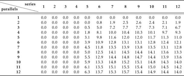
B.3 Methane production in Lisbon withη= 60%. . . 42
B.4 Methane production in Lisbon withη= 40%. . . 42
B.5 Incidence curves for methane production in Lisbon . . . 42
B.6 Methane production in Grenoble withη= 60% . . . 43
B.7 Methane production in Grenoble withη= 40% . . . 43
B.8 Incidence curves for methane production in Grenoble . . . 43
B.9 Methane production in Stockholm withη= 60% . . . 44
B.10 Methane production in Stockholm withη= 40% . . . 44
L i s t i n g s
I.1 Main Setup Script . . . 55
I.2 Function to calculate PV-IV curve . . . 60
I.3 Function to extrapolate values . . . 61
I.4 Extrapolation equation . . . 62
I.5 Function to fetch files . . . 62
G l o s s a r y
Energy content of hot water (Qtap) Means the product of the specific heat capacity of water, the average temperature difference between the hot water output and cold water input, and the total mass of the hot water delivered [1].
g-Value The g-value is a measure of how much solar heat (in-frared radiation) is allowed in through a particular part of a building. A low g-value indicates that a win-dow lets through a low percentage of the solar heat.
Load profile Means a given sequence of water draw-off[1].
Passive house A passive house is a building standard that is truly energy efficient, comfortable, affordable and ecolog-ical at the same time. They require less than 15 kWh/m2.year for space heating [2].
Peak temperature (Tp) Means the minimum water temperature,
ex-pressed in degrees Celsius, to be achieved during wa-ter draw-off[1].
Useful energy content (Qtap) Means the energy content of hot water, ex-pressed in kWh, provided at a temperature equal to, or above, the useful water temperature, and at water flow rates equal to, or above, the useful water flow rate [1].
Useful water temperature (Tm) Means the water temperature, expressed in de-grees Celsius, at which hot water starts contributing to the reference energy [1].
Useful water flow rate (f) Means the minimum flow rate, expressed in litres per minute, for which hot water is contributing to the reference energy [1].
G LO S SA RY
Water draw-off Means a given combination of useful water flow rate, useful water temperature, useful energy content and peak temperature [1].
Ac r o n y m s
η Faradaic efficiency (electricity-to-fuel). θ Incidence Angle on Solar Thermal Collectors. ηSTC Solar Thermal Collector efficiency.
A Diode factor.
a0 Intercept (maximum) of the collector efficiency. a1 Negative of the first-order coefficient in collector effi
-ciency equation.
a2 Negative of the second-order coefficient in collector efficiency equation.
b0 Parameter in 2nd degree polynomial equation for
IAM modifying factor..
b1 Parameter in 2nd degree polynomial equation for
IAM modifying factor..
CCU Carbon Capture and Utilization.
CSTB Scientific and Tecnical Centre for Building.
DAC Direct Air Capture. DHW Domestic Hot Water.
EC Electrochemical Cell.
EC-IV Electrochemical Cell - Current vs Voltage curve.
FF Fill Factor.
HE Heat Exchanger.
IMPP Current at maximum point.
IPH Photocurrent.
ISAT Reverse Saturation Current. ISC Short Circuit Current.
IT Global radiation incident on the solar collector (Tilted
AC R O N Y M S
IAM Incidence Angle Modifier.
LNEG Laboratório Nacional de Energia e Geologia.
MATLAB MATrix LABoratory.
PMPP Power at Maximum Point.
PV Photovoltaic.
PV-IV Photovoltaic panel - Current vs Voltage curve.
q Elementary charge.
QAuxHE Energy supplied by the auxiliary electric resistance in
the Heat Exchanger.
QAuxT Energy supplied by the auxiliary electric resistance in the Tank.
QDHW Energy demanded for Domestic Hot Water.
QSH Energy demanded for Space Heating.
QSTC Energy supplied by the Solar Thermal Collectors.
QTL Energy lost in the tank by thermal losses.
RS Series Resistance.
RSH Shunt Resistance.
SH Space Heating.
SNG Synthetic Natural Gas or Substitute Natural Gas. STC Solar Thermal Collector.
T Temperature.
Tamb Ambient Temperature. TC Cell temperature.
TESS Thermal Energy Systems Specialists. TRNSYS TRaNsient SYstem Simulation.
VMPP Voltage at maximum point.
VOC Open Circuit Voltage.
C
h
a
p
t
e
r
1
O b j e c t i v e s a n d Mo t i va t i o n
The energy crisis and global warming have become a serious issue and every year the annual global CO2 emissions increase and fossil fuel emissions account for about 91%
of total carbon dioxide emissions from human sources in 2014[3]. Solar Driven CO2 reduction has attracted more and more attention as the key technology to ensure a sta-ble supply of energy as renewasta-ble alternative to fossil fuels. Using methane as the end product of such system is very advantageous because of the already well-established in-frastructure for natural gas storage, distribution and consumption. The author takes also the responsibility to contribute to the transition to renewable energies sources otherwise future generations may not survive.
C
h
a
p
t
e
r
2
I n t r o d u c t i o n
2.1 Solar Fuels Generation
Carbon dioxide is a major greenhouse gas resulting from human activities. In the past centuries, utilization of carbon-rich fossil fuels - coal, oil and natural gas - has allowed an unprecedented era of prosperity and advancement for human development but also the increase of its concentration in the atmosphere from ~278 ppm before the industrial revolution to 403 ppm in 20161. The increase in CO2emissions arguably contributes to the increase in global temperature and climate change due to the greenhouse effect [4], posing a critical threat to the environment. Also, because of the highly dependence of fos-sil fuels for energy production worldwide and despite their considerable size, fosfos-sil fuels reserves are finite, limited and will, therefore, be increasingly depleted. A novel approach that is attracting a significant amount of interest is carbon capture and utilization (CCU), whereby captured CO2is converted into a diversity of chemical products including liquid hydrocarbons. The fuels produced via this route would replace an equivalent amount of fossil fuels, creating an almost closed loop of sustainable fuels utilization [5].
Because of solar energy intermittence, solar fuels generation is an attractive option with the advantage of capturing much of the photon energy in the bonds of portable and energy dense chemical species such as hydrogen or liquid hydrocarbons. This pro-cess can be achieved through the carbon-free hydrogen synthesis via water splitting and by electrolysis, thermochemical decomposition, photoelectrochemical dissociation via the carbon–neutral combination of water-splitting with electrochemical CO2reduction
reaction (CO2RR) to hydrocarbons fuels.
We will simulate methane generation in a flow electrochemical cell of water electroly-sis with electrochemical CO2RR, figure2.1, because of the direct 1-step fuels generation (equation2.2). Ideally, the reduction should yield to a single energy-rich compound. How-ever, selective methane production remains a challenging task at present due to multiple proton-coupled electron transfer steps involved in the reaction [6]. Despite the fact that this approach is still in the lab stage, it has been shown that methane could be obtained with high selectivity. The simulation is based on the work ofManthiram et al[7] on en-hancing the eletrochemical methanation of carbon dioxide in 1-step with a dispersible
C H A P T E R 2 . I N T R O D U C T I O N
nanoscale copper catalyst.
e
-H O CO +
+H O
CH +O
cathode
+
◄
+
-H+ ◄
H+ anode
H+ H
H
e
- ◄Figure 2.1: Scheme of the Electrochemical cell with the 1-step methane production
Another limitation of this process is the hydrogen competitive generation (eq. 2.1) with CO2 reduction (eq. 2.2), due to both reactions [8] having similar thermodynamic potential — 1.23 V for water splitting and 1.06 V for CO2reduction — consequently, we
have low faradaic efficiency for CH4generation.
2H2O
e−
→2H2↑+O2↑ ∆Go= 474.33kJ/mol (2.1)
CO2+ 2H2O
e−
→CH4↑+2O2↑ ∆Go= 818.18kJ/mol (2.2)
Various authors have noticed that the deactivation of copper electrodes occurs [9] after a few hours producing CH4. In this simulation work, we will consider that the EC
has stable performance throughout the year. However, to have an idea how electrode deactivation can affect solar methane production a lower faradaic efficiency was also considered. Thus, for voltage > 2.9V, the last value on the experimental data for CH4
faradaic efficiency from Manthiram et al., we will consider 60% and 40% efficiency for, respectively, good electrode performance and deactivation performance.
Although the low concentration of CO2in air for direct air capture (DAC) requires the treatment of high volumes, it has been investigated since half a century and has been applied in cryogenic oxygen separation plants [10]. DAC may use solid sorbents or aqueous basic solutions as capture media. Solid sorbents offer the possibility of low energy input, low operating costs and applicability across a wide range of scales but with the challenges that a very large structure has to be built at low cost while allowing the structure to be periodically sealed from the ambient air during the regeneration step and the conflicting demands of high sorbent performance, low cost and long economic life in impure ambient air. Aqueous sorbents offer the advantage that the contactor can operate continuously, can be built using cheap cooling-tower hardware and allows very long
2 . 2 . B U I L D I N G H E AT I N G R E Q U I R E M E N T S
contactor lifetimes despite dust and atmospheric contaminants. Disadvantages include the cost and complexity of the regeneration system and water loss in dry environments [11].
2.1.1 Integrated Photovoltaic-Electrochemical CO2Reduction
Some authors investigated the design and modulation of an offthe grid photovoltaic (PV) system for hydrogen production using methanol electrolysis achieving 24.38 g/m2PV
per day with PV array on a tilted surface [12]. It was reported in 2015 byGrätzel[13] workgroup a device driven solely by sunlight using water as electron source to reduce CO2 to carbon monoxide. They achieved a solar-to-CO efficiency of 6.5%. Meenesh R.
Singh et al[14] team showed in 2015 that solar-to-methane efficiencies for photovoltaic electrolyzers can operate at 7.2% with a thermodynamic limit at 41.8%, meaning that there is considerable opportunity for further improvement.
Some authors also analyzed methane production by PV panels, an electrolyser and Sabatier reactor and CO2/CH4conversion rate of 81% was obtained [15] and others
op-timized the Solargas process with different operating parameters [16]. However, this requires a Sabatier reactor and high pressure gases to achieve greater yield.Jordi Guilera et al.produced an article related to the economic viability of synthetic natural gas (SNG) production from power, carbon dioxide and oxygen to methane and concluded that the state of the art tecnology at the moment can produce SNG 2-7 times higher than conven-tional natural gas but this value could reduce up to 40 EUR/MWh, really close to the current price of conventional gas[17].
2.2 Building Heating Requirements
In 2016, the households or residential sector represented 25.4% of final energy con-sumption in the EU. Households use energy for various purposes: space and water heating, space cooling, cooking, lighting and electrical appliances. According to Eurostat [18], the EU-28 final energy consumption in the residential sector in 2016 for natural gas (NG) was 36.9%. In the residential sector, natural Gas plays an essential role in terms of space heating, water heating and cooking with, respectively, 43.4%, 47.9% and 33.1% of energy consumed for these end-uses (fig. 2.2). NG composition varies among different regions and suppliers but, generally, it consists 93.9% of methane [19], a compound with one carbon atom and four hydrogen atoms, 4.2% ethane, a compound with two carbons atoms and 6 hydrogen atoms, and a minor part of other gases. Because of solar energy’s abundance, methane high energy density of 50 MJ/kg [20] and an already existent infras-tructure for storage, transport and consumption, producing the so called "solar methane" is one of the most promising approaches to fill the need for energy.
C H A P T E R 2 . I N T R O D U C T I O N
Renewables and Wastes
Oil & Petroleum Products Solid Fuels
Natural Gas
Derived Heat
Electricity
Space
Heating CoolingSpace HeatingWater Cooking Lighting andappliances Other end uses
0% 10% 20% 30% 40% 50% 60% 70% 80% 90% 100%
Figure 2.2: Final energy consumption in the residential sector by type of end-uses for the main energy products, EU-28, 2016[18]
family concept building, figure2.3, with a central heating system connected to a storage tank that provides the necessary heating requirements for Space Heating (SH) and Do-mestic Hot Water (DHW). It has Solar Thermal Collectors (STCs) to provide part of the heating needs and if the heating needs cannot be fulfilled by the STCs, then they are sat-isfied by the combustion of stored methane synthesized by the PV-powered electrolyzers. We will use MATLAB software to simulate a conversion system that uses solar energy from PV panels into electricity to power a 1-step reaction in a electrochemical (EC) flow cell(s), using CO2and water as feedstock, in an attempt to show the possible viability of such system integrated in future houses.
O 2 CO -free air2
CO2 E-Chemical cells split
CO + 2H O ↔ CH + 2O
Central heating
uses natural gasto circulate hot water
Storage of gas fuels for cooking and central heating
CO Direct Air Capture2
unit filters CO2 from the building air exhaust
Solar PV tiles power electrolyzers with DC
Figure 2.3: Illustration of the concept house. The energy harnessed by PV panels powers the electrolyzers to produce methane that is stored for future use.
2 . 2 . B U I L D I N G H E AT I N G R E Q U I R E M E N T S
Figure 2.4: TRNBuild Interface
The aim of the present work is to investigate how solar methane can be produced in residential buildings for in house combustion to satisfy heating needs. For this, three locations will be considered: Lisbon in Portugal, Grenoble in France and Stockholm in Sweden. The building walls and windows specifications were built according to the space heating needs for each location. In Lisbon and Grenoble, a passive house with 15 kWh/m2.year of space heating was studied. In order to test a building less efficient, we also considered one with higher SH energy demand, 100 kWh/m2.year, only for Grenoble and Stockholm. Another variable under study is STCs area where commercially available STCs were considered and we tested two different areas, 4 and 6 m2.
C
h
a
p
t
e
r
3
A r c h i t e c t u r e o f t h e S y s t e m
3.1 Software used
3.1.1 TRNSYS
TRNSYS is a complete extensible simulation environment for the transient simulation of systems, including multi-zone buildings. It was originally developed by the Solar Energy Laboratory in University of Winsconsin, Madison, USA[trnsys_ref] but then it was also developed on continuously partnership with TRANSSOLAR Energietechnik GmbH1, Thermal Energy Systems Specialists (TESS)2and Scientific and Tecnical Centre for Building (CSTB)3. The most recent version is 18 released in 2017 but version 16 was used for this work from license number available from Laboratório Nacional de Energia e Geologia (LNEG), Portugal.
TRNSYS is used by engineers and researchers around the world because of its versatil-ity and allows to validate new energy concepts, from simple domestic hot water systems to the design and simulation of buildings and their equipment, including occupant be-haviour and alternative energy systems (wind, solar, photovoltaic, hydrogen systems, fuel cells).
TRNSYS consists of a suite of programs: the TRNSYS Simulation Studio, which is the main visual interface, the simulation engine (TRNDll.dll), its executable (TRNExe.exe) and the building input data visual interface (TRNBuild.exe).
A TRNSYS project is typically setup by connecting components graphically in the Simulation Studio, by drag-and-dropping components in the workspace, connecting them together and setting the global simulations parameters. Each component, also called type, is described by a mathematical model in the TRNSYS simulation engine and has a set of matching proforma’s in the simulation studio. The proforma has a black-box description of a component: inputs, outputs and parameters that can be personalized for the specific simulation environment [21].
C H A P T E R 3 . A R C H I T E C T U R E O F T H E S YS T E M
3.1.2 MATLAB
MATLAB (MATrix LABoratory) is a tool for technical computing, computation and visualization in an integrated environment and is developed by The MathWorks4. The license used was from Faculdade de Ciências e Tecnologias da Universidade Nova de Lisboa. Various scripts were created to automatize the processing and analysation of the TRNSYS simulation studio data outputs and the parameters used can be found in the annexI.
3.2 Methodology
The methodology used for this thesis is described in figure3.1.
PV data from TRNSYS
IV curve characteristicsHouse needs
data from TRNSYS
Energy Space Heating
Energy Auxiliar
Energy Solar Thermal Collector
Energy Domestic Hot Water
Energy Thermal Losses
MATLAB Analysis
Methane Volume Hydrogen Volume Oxygen Volume
Excel Analysis
Results for
different electrode performance different solar colectors areas different buildings configurations
different locations
1 Year data
Figure 3.1: Scheme of the methodology used
In order to test this concept, three locations were chosen: Lisbon in Portugal (N 38º 43” W 9º 9”), Grenoble in France (N 45º 22” E 5º 20”) and Stockholm in Sweden (N 59º 21” E 17º 57”). We also tested the house needs for space heating and domestic hot water consumption of two type of homes: a passive house with 15 kWh/m2.year on space heating (SH) consumption for Lisbon and Grenoble and a more standard house with 100 kWh/m2.year SH consumption for Grenoble and Stockholm. Because we also wanted to see the influence of different solar thermal collectors areas on our building, we also tested for STCs areas of 4 and 6 m2. To test the performance of our Electrochemical cell (EC) when considering electrode deactivation for voltage >2.9V, we will consider a faradaic efficiency of 60% and 40%.
4https://www.mathworks.com/
C
h
a
p
t
e
r
4
D i s c u s s i o n a n d r e s u lt s
4.1 TRNSYS Parameters
In this chapter, the building description and the most important TRNSYS files param-eters are defined, everything not listed remained as default in the TRNSYS environment. The output values are saved at each instance of the simulation in a text file which are then processed by MATLAB and Excel.
4.1.1 Main Project
Each TRNSYS simulation ran for 8766 hours, simulating 1 year, with a time step of 90 seconds and successive substitution as the solution method. Tolerance integration and convergence errors are both set to 0.001. The main project is represented in fig. 4.1and is divided in 4 sections: the building itself and its vital connections (red lines), space heating calculation loop (purple lines), the solar collector loop (dark blue lines) and the domestic hot water loop (green lines). The way this simulation works is by every section giving or taking heat from the tank (type60d) which is fed by the solar collector. If any additional heat is needed, the tank activates an electric resistance that provides the auxiliary heat required (Qaux) which is then printed at every timestep to a file. Outside the TRNSYS environment, Qaux is then converted to the equivalent quantity of methane as it was combusted in a boiler with an efficiency of 90%.
In order to store heat in the form of hot water, we simulated the use of tank (type60d) with 2 heat exchangers, one for space heating and another for the solar collector loop and an electric auxiliary heater that kicks in when the STCs are not gathering enough heat to suppress the house heating needs. A second electric auxiliary was exclusively used for space heating requirements. Also, to foresee domestic hot water (DHW) consumption we used eight Time Dependent Forcing Functions, 4 for Water Draw (type14b) and another 4 for water Temperature (type14e), with a water load profile M from European Journal [1] with conjunction with a diverter (type11b) and a tee piece (type11h) to work as a mixing valve for hot and cold water to get the desired temperature for domestic water use.
C H A P T E R 4 . D I S C U S S I O N A N D R E S U LT S
Building Connections Space Heating
Solar Thermal Collector Loop Domestic Hot Water Loop Calculations
Outputs
Figure 4.1: Printscreen from TRNSYS Studio environment. Red lines represent the build-ing connections, dark blue lines represent the solar collector loop, green lines represent the DHW loop, light blue lines represent calculations, grey lines represent outputs
METEOTEST1, the license number was used from LNEG, referring to the radiation data from 1991-2010 and temperature and other parameters from 2000-2009. Three different locations in Europe were used for this work: Lisbon in Portugal, Grenoble in France and Stockholm in Sweden.
For this work, we simplified the combustion of CH4system and used the tank’s
auxil-iary heating rate output value to mimic the burning, similar to what a boiler would burn natural gas (94% is methane) to heat water into the tank and a 90% conversion efficiency was considered. The reference building is defined in the following chapter, including architectural design and orientation as well as constructive descriptions of all building elements such as walls, floors, windows and roof.
1https://meteotest.ch/
4 . 1 . T R N S YS PA R A M E T E R S
4.1.1.1 Building Parameters
For this work, it was used the building project helping assistance guide for multi-zone buildings from TRNSYS to build our test building in two different conditions: bui15 and bui100 related to a building that consumes 15 kWh/m2year and bui100 for 100 kWh/m2 year, respectively, in space heating. This multi-zone building component model (type56) is a non-geometrical balance model with one air node per zone, representing the thermal capacity of the zone air volume and capacities which are closely connected with the air node (furniture, for example). Thus the node capacity is a separate input in addition to the zone volume [22].
The reference buildings are based on theTask 32 for project report A2 of subtask A: The Reference Heating System, the template Solar systemmade by Solar Heating & Cooling Programme, International Energy Agency (SHC). The building naming references to their heating loads, such as 15 and 100 kWh/m2.year. Both have the same architectural design but different insulation thickness for distinct locations as described in figure4.2and table
4.1.
Figure 4.2: Scheme of the building dimensions
The building is a two storey housing, with effective floor area as 70 m2per store. The window area on the South, North, West and East façades are, respectively, 25%, 6%, 10% and 10%. Both floors are simulated as one common thermal zone with 200m2of internal walls and a total volume area of 364 m3. The house used in this work was made using TRNSYS multizone building project assistant and was simplified in terms of dimensions and number of zones. The various materials, layer thicknesses and energy performance describing the buildings bui15 and bui100 are listed in Table4.1.
C H A P T E R 4 . D I S C U S S I O N A N D R E S U LT S
Table 4.1: Construction building elements for 15 and 100 kWh/m2.year houses. L15 is for Lisbon, G15 and G100 is for Grenoble, and S100 is for Stockholm
Assembly Layer layer thickness Conductivity Capacity Density U-Value construction
L15 G15 G100 S100 L15 G15 G100 S100
m m m m kJ h-1m-1K-1 kJ Kg-1K-1 kg m-3 W m-2K-1
Ground Floor Wood 0.015 0.015 0.015 0.015 0.5400 2.50 600
0.173 0.439 0.158 0.225 Plaster Floor 0.060 0.060 0.060 0.060 5.0400 1.00 2000
XPS 0.200 0.070 0.220 0.150 0.1332 1.45 38 Concrete 0.150 0.150 0.150 0.150 7.5600 0.80 2400
Total 0.425 0.295 0.445 0.375
External Floor Plaster Inside 0.015 0.015 0.015 0.015 2.1600 1.00 1200
0.178 0.235 0.333 0.228 Viertl brick 0.300 0.210 0.210 0.300 2.5200 1.00 1380
EPS 0.200 0.150 0.100 0.150 0.1440 1.45 17 Plaster Outside 0.003 0.003 0.003 0.003 2.5200 1.00 1800
Total 0.518 0.378 0.328 0.468
Roof Gympsumboard 0.025 0.025 0.025 0.025 0.7600 1.00 900
0.207 0.317 0.291 0.291 Plywood 0.015 0.015 0.150 0.015 0.2916 2.50 300
Rockwool 0.150 0.090 0.100 0.100 0.1296 1.03 60 Plywood 0.015 0.015 0.150 0.015 0.2916 2.50 300
Total 0.205 0.145 0.425 0.155
Internal Wall Clinker Brick 0.200 0.200 0.200 0.200 0.8280 0.92 650 0.962
Table 4.2: Thermal properties of windows for the 15 and 100 kWh/m2.year building
Location Bui. Heating Load Uwindow g-Value Uframe Construction Window ID
kWh m-2year-1 W m-2K-1 kJ h-1m-2K-1 mm
Lisbon 15 5.74 0.87 8.17 4/16/4/16/4 1001
Grenoble 15 2.83 0.755 8.17 4/16/4 1202
Grenoble 100 5.74 0.87 8.17 4/16/4/16/4 1001
Stockholm 100 2.83 0.755 8.17 4/16/4 1202
4.1.1.2 Storage Tank
The type 60d is used to simulate the storage tank and a scheme can be found in figure
4.3. Two heat exchangers (HE) are used to simulate the solar collector heat input and the heat output for the space heating loop. For the domestic hot water loop, we used the output of the tank itself. Also, at times when the heat provided by the solar collectors is not enough, a heat resistance provides the auxiliary heating requirements to satisfy the energy needs.
The tank volume changes following a relation of 82.5 m3per m2of collector [23]. The tank height is a fixed value of 1.25 meters for the two cases of different solar collector area. Water is the fluid used for the tank and heat exchanger (HE) 2. For the HE 2, it enters the Tank at a fixed temperature of 30ºC meaning that from the higher output temperature needed (>50ºC), for space heating, the water doesn’t transfer all its heat to the environment and instead the water stays warm. For the heat exchanger 1, a water based solution of 75% ethylene-glycol is used. The tank loss coefficient is given by 3 kJ h-1m-2K-1 and a fraction timestep of 6 is used on the tank.
4 . 1 . T R N S YS PA R A M E T E R S
HEAT EXCHANGER 1 SOLAR COLECTOR HEAT EXCHANGER 2 SPACE HEATING
INLET 1
DOMESTIC HOT WATER OUTLET 1
DOMESTIC HOT WATER
0.6 m
1 m
TANK AUXILIARY HEATER
HEAT EXCHANGER AUXILIARY HEATER
0.9 meters
0.5 m
Figure 4.3: Scheme of the storage tank used and its inputs, outputs, heat exchangers and heights. Blue arrows represent cold fluid while red arrows represent hot fluid.
4.1.1.3 Solar Collector Loop
From fig. 4.1in dark blue lines are represented the solar collector loop and its com-ponents: type109 (Weather), type3 (Pump), type2 (On-Offswitch), solar collector type1 and Tank type60d. However, to test the different collector area, modifications have to be made the tank size, pump mass flow inlet, heat exchanger area and length, according to reference [23] and are presented in table4.3.
The tank volume size must be 82.5 m3per m2of collector, the pump massflow is given by 0.02 kg s-1per m2of STC2, the heat exchanger surface area is give by 0.2 m2per m2 of collector and the heat exchanger length is given by the area of a cylinder in equation
4.1.
A=π·D·L (4.1)
• A, the total surface area of the heat exchanger in m2
• D, the diameter = 0.012 m
• L, length of the heat exchanger in meters
C H A P T E R 4 . D I S C U S S I O N A N D R E S U LT S
Table 4.3: TRNSYS parameters modification when changing the collector area
Collector Area Mass Flow Rate
Tank Volume
Heat Exchanger Length
Total Surface Area of Heat Exchanger
m2 kg hr-1 m3 m m2
4 288 330 21.20 0.8
6 432 495 31.85 1.2
The collector is a flat plate type with aperture area of 2.0 m2and displayed in table
4.4are the values inserted in the component type.
The collector was positioned with a slope of 45º, 20% ground reflectance with the type using optical mode 2, meaning that the incidence angle modifier for adjustment is calculated following a second order quadratic function. The fluid used was a water based solution of 75% ethylene glycol with a specific heat of 2.93 kJ kg-1 m-2 K-1. The solar fraction is given by eq. 4.2and the solar collector thermal efficiency is given by equation
4.3. The intercept efficiency is corrected for non-nomal solar incidence by a modifying factor4.4with b0= 0.2 and b1= 0.
SolarFraction= QST C−QT L QSH+QDHW
·100 (4.2)
ηST C =a0·IAM−a1
∆T
IT
−a2
(∆T)2
IT
(4.3)
IAM= 1−b0·S−b1·S2 with S=
1 cos(θ)−1
!
(4.4)
For the control of the solar loop, the upper input temperature (THigh) is given by the
Table 4.4: Reference collector performance parameters from datasheet
a0 a1 a2
kJ hr-1m-2K-1 kJ hr-1m-2K-2
0.740 1.520 0.005
collector outlet temperature, the lower input temperature (TLow) is given by the tank
temperature at outlet of heat exchanger 1 and the monitoring temperature for high limit cut out checking is given by the temperature of outlet flow 1, as described in the storage tank figure4.3. The lower dead band dT is given by 2K and the upper dead band dT by 10K. If the controller was previously ON and the lower dead band is smaller than the different of THigh-TLow, then the controller remains ON. Otherwise it turns OFF. If the controller was previously OFF and the upper dead band value was smaller than THigh
-TLow, then the controller turns ON. Otherwise it remains OFF. Consult AppendixAfigure
A.2for a scheme [22].
The monitoring temperature makes sure that no matter the result of the controller switch, the temperature never exceeds 100ºC for safety issues. Probable causes are col-lector stagnation and storage tank protection where the pump is not allowed to run if
4 . 1 . T R N S YS PA R A M E T E R S
the tank temperature is above some prescribed limit. More details can be found in the reference [22] page 15.
4.1.1.4 Space Heating Loop
The space heating loop is represented with purple lines in fig. 4.1. We use 65ºC as the setpoint temperature from the outgoing HE2 of the tank and a return temperature of 30ºC. Knowing the heating rate required in the building to maintain 20ºC, we calculate what is the flow rate necessary with equation4.5.
˙
Q= ˙m·Cp·(Tsetpoint−Treturn) (4.5)
• ˙Q, heating rate in kJ hr-1
• ˙m, mass flow rate in kg hr-1
• Cp, specific heat for water in J kg-1K-1
• Tsetpoint, exiting temperature in HE2 set point in ºC
• Treturn, return temperature from the building central heating
Because there are situations when the tank can’t give enough heat to maintain outgo-ing temperature of HE2 as 65ºC, a electric resistance will be simulated exclusively for the HE2. Using the same eq. 4.5, we can simulate the extra heating rate we must deliver to maintain the 65ºC set point but now the return temperature is given by the actual temperature exiting the heat exchanger 2 instead of the fixed 30ºC.
4.1.1.5 Water Draw Profile
Based on EU directive Number 814/2013 [1] and to simulate the usage of water in a single house family which uses in average 300 liters per day with different water draw-offs (tapping), the load profile M3was used. This was achieved in the TRNSYS environment using the 2 sets of four type14 components. One set simulates the profile mass flow and the other simulates the desired temperature for 0h-9h, 9h-15h, 15h-20h, 20h-24h time-frames of the day. The output connections "instantaneous water draw" from all 8 types are connected to the Diverter inputs "inlet mass flow rate" and "Set Point Temperature", respectively. If the "average water draw" output was used instead of the instantaneous water draw, the water used daily would be 213 liters instead of 315 liters. This is because the small timestep used during the simulation (90s) and the intervals of time in the load profile do not coincide, making TRNSYS average the value in the end of the simulation timestep instead of the actual time in the load profile.
The tapping cycle is defined as a set of the following parameters: heat demand per tapping (Qtap [kWh]), minimum volume flow rate (f [l/min]), minimum temperature
C H A P T E R 4 . D I S C U S S I O N A N D R E S U LT S
(Tm[ºC]) and peak temperature (Tp [ºC]). Since the implementation in TRNSYS of this
load profile requires different input values such as inlet and outlet temperatures and the mass flow rate, the profiles are recalculated based on theEnergy Labelling of Custom Built Systems, Deliverable D3.2by Sebastian Bonk in QAiST4in Table4.5and presented in AppendixATableA.2.
Table 4.5: Recalculations used to implement load profile on TRNSYS
Value Calculation
Inlet Temperature (TCW) 10 ºC
Outlet Temperature (TL) During the tapping: max(Tm,Tp)
Mass Flow Rate (mdot) mdot=
Qtap
N·dt·cp·(TL−TCW)
With:
• N = discrete number of time steps
• dt = 90 seconds
• cp = 4.187 kJ kg-1K-1
Because the tank setpoint temperature is at 55ºC, a mixing valve is required to mix cold and hot water for domestic use at 30-45ºC (according to the load profile temperature requirements). This valve is simulated using two types 11 components: one as a temper-ing valve and another as a tee piece. The inlet temperature to mix the hot water is 10ºC. The types 14, simulating the load profile, connect to the diverter giving ON/OFF status and temperatures setpoints for the DHW. The temperature from storage tank outlet 1 connects to the heat source temperature of the diverter which then feeds back to the tank providing a flow rate and temperature for the tank inlet 1. Also, the diverter and the stor-age tank outlet 1 feeds the tee piece the flow and temperature of the water appropriated now for domestic use.
4.1.2 Photovoltaic project
In another TRNSYS project, a simple PV simulation system was used with photo-voltaic panels (type94a) and the Data Reader and Radiation Processor component to read the weather data. Because of the architecture of the system used, the type94a didn’t give all the outputs we required to make our Current-Voltage (IV) calculations curves. Using Compaq Visual Fortran Edition 6.6.B, license made available from LNEG, we altered the Proforma file so that we could get more outputs from our photovoltaic panel component, such as reverse saturation current dependent on temperature (ISAT), photocurrent
depen-dent on insolation (IPH), cell temperature (TC), open circuit voltage (VOC), short circuit
4http://www.qaist.org/
4 . 2 . M AT L A B S YS T E M
current (ISC), fill factor (FF), series resistance (RS), array voltage, array current, array
power, power at maximum point (PMPP), voltage at maximum point (VMPP), current at
maximum point (IMPP), number of cells (NS), number of modules in series (NMS), number of modules in parallels (NMP). This new type was called type161.
Each TRNSYS simulation ran for 8766 hours, simulating 1 year, with a time step of 1 hour and successive substitution as the solution method. The new component, type161, cell parameters were based on SUNPOWER5B50 Solar Cell G in mono crystalline silicon and the full data sheet can be found in appendixAfig. A.3. The cell parameters are in table4.6.
Table 4.6: Electrical characteristics parameters of solar cell used from SUNPOWER, B50 Solar Cell G in mono crystalline silicon at standard test conditions: 1000W/m2, AM 1.5 and cell temp 25ºC
VOC ISC VMPP IMPP PMPP Efficiency
V A V A W %
0.664 5.72 0.557 5.33 2.97 20
4.2 Matlab System
4.2.1 PV-IV script
For each timestep of 1 hour in the TRNSYS simulation PV project, the functionI.2in annexIwas created in MATLAB to calculate the PV-IV curve given the parameters: VOC,
IPH, ISAT, TAMB, NS, NMS, NMP, RS, RSH, A. The function can be summarized in:
• Start by creating a array sized 150 from 0 to VOC and the start current i=0.
• A loop is created for each array element V(i).
• For each loop (idx), a current value I(idx) is calculated with equation4.6using the current from previous iteration (i).
I(idx) =IPH−ISAT·exp V
+ (i·RS)·q
A·k·T amb·NS !
−V+ (i·RS)
RSH
(4.6)
• In the end, the Tension array is multiplied by the number of cells and modules in series used in the simulation. The Current vector is multiplied by the number of modules in parallels.
C H A P T E R 4 . D I S C U S S I O N A N D R E S U LT S
4.2.2 Methane production script
TRNSYS outputs from the photovoltaic project were saved in a .txt file and imported to MATLAB. These outputs are the characteristics parameters from a photovoltaic crys-talline cell, that allow the construction of IV graph. The core script of this work is described in the scheme in the figure4.4.
Iop x 3600
F x 8
molesCH = (A)
molesCH x R x Tamb
Pressure x ƞCH
VolumeCH = ▼ (C)
Next T
24.2 x 2 x molesCH + molesH
VolumeO = (D)
2
(
▼ ▼(
molesH x R x Tamb
Pressure x
ƞ
HVolumeH = (E)
Iop x 3600
F x 2
molesH = (B)
PV - IV Curve EC - IV Curve
Intersection
Vop Iop
CH FaradaicCurve
H Faradaic
Curve Intersection
Intersection
ƞCH = 60% ƞH = 20%
If Vop > VEC,last
ƞCH
ƞH
ƞCH = 40% ƞH = 5%
► ◄ ▼ ▼ ▼ ▼ ▼ ▼ ► ► ▼ ► ▼ ▼ ◄ ► ► ▲ ► ◄ ▼ ▼ ▼ ► ▲ ◄ T ▼ ▼
First T = 1
▼
Figure 4.4: Scheme for the main MATLAB script. This is a loop for every hour of the yearly simulation, starting at iteration T=1. Vop in Volts, Iop in Amperes, F = 96485 Coulomb, R=0.082 atm/mole K, Tamb=298 K, Pressure = 1 atm.
The script calculates the methane produced hourly from the intersection of the pho-tovoltaic panel’s IV curve with the IV curve of a dispersible nanoscale copper catalyst[7] from Manthiramet alwork. His group characterized this EC and the following curves from his article were used: Density of current vs Potential ([7] figure 2.A), CH4Faradaic Efficiency vs Potential ([7] figure 2.B) and H2Faradaic Efficiency vs Potential ([7] figure 2.D). Another assumption that was made for this simulation was that the performance of the electrodes was constant. To take deactivation into account a lower Faraday efficiency of 40% was considered. This deactivation is due, for example, to degradation of the n-Cu/C catalysts during the year. The size of the electrodes used in this thesis is given by 50cm x 50cm, which means a area equal to 0.25 m2.
As shown in appendix B fig. B.17, Manthiram et al. experimental results Current Density vs Potential only reached -1.45 V vs RHE. As this data represents the potential
4 . 2 . M AT L A B S YS T E M
of the cathode, we have estimated the whole cell potential adding 1.5 V for the anode reaction (oxygen evolution) considering an overpotential of ca. 0.3V. However, in some cases studied in the simulations, the voltage from PV-IV panel would be higher than 2.9 V as shown in4.5. Assuming a constant selectivity of the reaction in this potential range, a fitting of the EC-IV and extrapolation until 4 V following equationy=a·eb+xwas created to take into account situations where the PV-IV wouldn’t intersect with the EC-IV data. The code can be found in annexII.3. Also, in our calculations, CO2and water will never
be the limiting factor in the reactions and only the power produced in the PV panels will limit our solar methane generation.
Pmpp
Real PV-IV Curve
EC-IV extrapolation
Matched PV Curve
Experimental EC
Real PV-IV Curve
EC-IV extrapolation
T = 83
T = 231
EC-IV experimental curve EC-IV experimental curve
Figure 4.5: PV-IV intersecting with EC-IV for iteration T = 83 and T = 231 for the example case PV in Lisbon with 5 cells in series and 4 modules in parallel.
Ideally, the optimal point for intersection would be at Pmppof the PV-IV curve.
How-ever, due to actual irradiance and temperature being the main parameters affecting the current variation, it is not easy and straightforward to find the optimal combination of cells and modules. A battery of tests with different configurations ranging from 1x1 (1 cell in series and 1 module in parallel) up to 12x12 (12 cells in series and 12 modules in parallel) was produced for the three different locations and then ran in the MATLAB script to oversee which configuration would produce more methane. The results are presented in appendix B. To have an idea on how the results deviate from the EC- IV experimental data, we calculated the percentage of incidence of those intersections on the extrapolated curve and found it satisfying considering results with less than 20% of intersections.
In the following code, the operational Current (IOP), that resulted from the intersec-tion of PV-IV with EC-IV, is multiplied by dt which represents 3600 seconds because each PV-IV curve is from 1 hour data. Because there are 8 electrons involved in CO2RR
ca-thodic reaction, eq.4.8, each mole of CH4is given by dividing the product of Operational Current with dt per the product of Faraday constant with 8 (fig. 4.4equation A).
C H A P T E R 4 . D I S C U S S I O N A N D R E S U LT S
3 VolumeCH4(a) = (moleCH4 * R * Tamb)/Pressao * etaCH4(a); % PV=nRT 4 Metano = Metano + VolumeCH4(a);
By using the Ideal Gas Law PV =nRT (fig. 4.4eq. C), we can calculate the methane volume in liters produced for each hour. The value is then added to a summation variable to be printed at the end of the loop. The same principle is applied for the hydrogen production with the respective faradaic efficiency (fig.4.4equation B and E). The volume of oxygen produced at the anode (eq.4.7) can be calculated in the same way considering the total number of moles, formed in the reaction producing methane, and in the water electrolysis reaction (fig. 4.4equation D).
Anodic: 2H2O→4H++ 4e−+O2↑ (4.7)
Cathodic:CO2+ 8H++ 8e−→CH4+ 2H2O
2H++ 2e−→H2↑ (4.8)
GlobalReaction:CO2+ 2H2O→CH4+ 2O2 (4.9)
4.3 Results
The results from the battery of tests for different PV panels configurations are pre-sented in appendix B and the configuration chosen for each location took into consid-eration two parameters: maximum CH4 production and less than 20% of results from the extrapolation curve. The latter percentage was arbitrarily chosen to minimize the number of intercepts with the extrapolation curve to lead to a conservative assumption of methane production.
In table4.7 is summarized the production of Methane, Hydrogen and Oxygen for different locations taking into consideration that no electrode deactivation occurred. The columns of production are based on products produced per square meter of PV area per year. One module is a number of cells connected in series (NS) and 1 PV unit is a
number of modules connected in parallel (NMP) as represented in the fig4.6. We have
also designated 1 EC unit as one electrode with geometrical area of 0.25 m2.
Table 4.7: Methane, Hydrogen and Oxygen productions in Lisbon, Grenoble and Stock-holm with electrocatalyst of 0.25 m2no deactivation considered. NTP conditions.
Location Ns Nmp PV Area
CH4 prod.
H2 prod.
O2 prod.
Extrapolation Incidence Curve m2 kg/m2PV.y kg/m2PV.y kg/m2PV.y %
Lisbon 12.0 12.0 2.250 16.8 2.8 223.1 17.9
Grenoble 10.0 12.0 1.875 14.7 2.4 195.4 14.9
Stockholm 10.0 12.0 1.875 12.5 2.1 166.2 12.0
4 . 3 . R E S U LT S
Figure 4.6: Scheme for the designated "PV Unit". In this example, 1 PV Unit consists of 4 cells connected in series are called 1 module. 3 Modules connected in parallel are called 1 PV Unit.
AppendixA and fig.A.1 show the radiation hitting the three different locations in study and Lisbon has the highest incidence with a mean radiation of 722 kJ/hr.m2 fol-lowed by Grenoble with 545 kJ/hr.m2 and finally Stockholm with 400 kJ/hr.m2. As expected from this results, Lisbon would give a greater yield followed by Grenoble and Stockholm. Also, because of the higher irradiance in Lisbon and the temperature and ir-radiance being the actual parameters affecting methane production, we have more PV-IV EC-IV intersections in the extrapolation curve in relation to the other locations.
4.3.1 Influence of electrodes deactivation
To consider the effect of electrode deactivation, a faradaic efficiency of 40% was used when we get values on the extrapolation curve (>2.9V). As expected, a decrease in pro-duction of 33% is obtained, as presented in figure4.7.
4.3.2 Influence of different space heating consumption
C H A P T E R 4 . D I S C U S S I O N A N D R E S U LT S
Figure 4.7: Left: Daily Methane Production Right: Yearly Methane Production
Jan. Feb. March April May June July Aug. Sept. Oct. Nov. Dec.
0
100
200
300
400
500
600
700
800
900
H
e
a
ti
n
g
R
e
q
u
ir
e
m
e
n
ts
(
k
W
h
/m
o
n
th
)
QAuxT
QSolarCollector QSpaceHeating QDomesticHotWater QThermal Losses QAuxHE
Figure 4.8: Monthly heating requirements for Grenoble building 15 kWh/m2.year and STC 6 m2
Increasing the space heating needs to 100 kWh/m2 implies an increase in 20% of the fraction of QAux supplied. The heating load max is the maximum amount of energy supplied for space heating at a given moment. The buildings were designed to be as close as 15 and 100 kWh/m2.year in space heating needs however it was not possible to reach exactly those requirements and so the effective space heating demand is presented in the table4.8. Increasing in 460% the space heating demand provoked a demand for methane
4 . 3 . R E S U LT S
-50
0
50 100 150 200 250 300 350 400
-10
0
10
20
30
40
C
H
4
R
e
q
u
ir
e
d
(
k
g
)
Time (Day)
Figure 4.9: Daily methane requirements for Grenoble building 15 kWh/m2.year and STC 6 m2
increase in 360% for STC 4 m2and almost 400% for STC 6 m2.
One PV unit is equal to 10 cells connected in series and 12 modules in parallel with a total area of 1.875 m2and one EC unit equals to a electrochemical reactor cell with an electrode geometrical area of 0.25 m2. Using 1 Unit of PV and EC the system produces 27.7 and 18.5 kg of methane withη = 60 and 40% and taking into consideration a 90% methane combustion efficiency to heat. To fulfil the CH4requirements we would need several of those units, as represented in table4.8. The auxiliary heating fraction is give by eq 4.10 and the methane needed for each situation takes into consideration a 90% combustion efficiency as it would burn in a conventional boiler.
Table 4.8: PV and EC area needed for Grenoble buildings. One PV Unit equals to 10 cells connected in series and 12 modules in parallel with a total area of 1.875 m2. Solar Fraction + QAux Fraction = 100%
Building STC η
Area PV needed Area EC needed Number of EC & PV units
CH4
needed
CH4
gen-erated per PV Unit Solar Fraction Fraction QAux Heating Load Max
Effective
Space Heat-ing demand m2 % m2 m2 kg/y kg/y % % kWh kWh/m2.y
bui15
4 60 17.8 2.4 9 262 27.7 41.0 59.0
50.0 18.5
40 26.5 3.6 14 18.5
6 6040 15.723.5 2.13.1 138 232 27.718.5 48.0 52.0
bui100
4 60 81.7 10.9 44 1205 27.7 14.0 86.0
144.0 103.5
40 122.1 16.3 65 18.5
6 6040 77.6116.0 10.415.5 4162 1145 27.718.5 18.0 82.0
FractionQAux=(QAuxT+QAuxHE2)
C H A P T E R 4 . D I S C U S S I O N A N D R E S U LT S
4.3.3 Influence of different building location
Comparing Lisbon to Grenoble bui15, the number of Units needed decreased to fea-sible numbers with a best scenario requiring 7.5 m2of PV area and 8.4 m2of electrode geometrical area. However, when changing the location of the bui100 from Grenoble to Stockholm, the units needed increased from the minimum of 41 in Grenoble to a min-imum of 53 in Stockholm, which represents a PV panel area of almost 100 m2. In a situation with STC 6 m2and not considering electrodes deactivation on the EC, we can achieve the best result among te worst scenarios of about 95.3 m2PV area. The worst case scenario in Stockholm requires more PV panel area than the useful area of the building (140 m2).
Table 4.9: PV and EC area needed for Lisbon building. One PV Unit equals to 12 cells connected in series and 12 modules in parallel with a total area of 2.25 m2. Solar Fraction + QAux Fraction = 100%
Building STC η
Area PV needed Area EC needed Number of EC & PV units
CH4 needed
CH4 gen-erated per PV Unit Solar Fraction Fraction QAux Heating Load Max
Effective
Space Heat-ing demand m2 % m2 m2 kg/y kg/y % % kWh kWh/m2.year
bui15
4 60.0 9.9 1.1 4 166.6 37.9 58.7 41.3
60.0 14.8
40.0 14.8 1.6 7 25.3
6 60.040.0 7.511.3 0.81.3 35 127.0 37.925.3 68.5 31.5
Table 4.10: PV and EC area needed for Stockholm building. One PV Unit equals to 10 cells connected in series and 12 modules in parallel with a total area of 1.875 m2. Solar Fraction + QAux Fraction = 100%
Building STC η
Area PV needed Area EC needed Number of EC & PV units
CH4 needed
CH4 gen-erated per PV Unit Solar Fraction Fraction QAux Heating Load Max
Effective
Space Heat-ing demand m2 % m2 m2 kg/y kg/y % % kWh kWh/m2.year
bui100
4 60 98.6 13.1 53 1236.7 23.5 10.4 89.6
157.0 101.7
40 147.5 19.7 79 15.7
6 6040 95.3142.5 12.718.9 5176 1195.1 23.515.7 13.4 86.6
From fig. 4.11we can observe that Stockholm lacks consistency, only producing in the summer months because that location has, in average, less than fifty hours of sunlight in january and in the peak of summer it has more than 300 hours (table4.11). During those short sunlight in winter, the sun never reaches the altitude of the orientation of the PV panel (33º), because of that, no direct radiation is is focusing on the PV panel and consequently, no methane generation during the cold months. From table4.11 and fig.
4.10we can understand how the space heating demand increases in the winter but for those months, STCs and methane generation is limited by the number of sunshine hours provoking a increase by at least ten-fold compared to Lisbon in PV and EC units needed.
4 . 3 . R E S U LT S
0 2000 4000 6000 8000 10000 -15 -10 -5 0 5 10 15 20 25 30 35 bui15_Grenoble 0 1 2 3
0 2000 4000 6000 8000 10000 -5 0 5 10 15 20 25 30 35 40 bui15_Lisbon 0 1 2 3 4
0 2000 4000 6000 8000 10000 -15 -10 -5 0 5 10 15 20 25 30 35 Temp. House Temp. Ambient
Space Heating Demand
Time (hour) Temperature (ºC) bui100_Grenoble -1 0 1 2 3 4 5 6 7 8 9
0 2000 4000 6000 8000 10000 -20 -15 -10 -5 0 5 10 15 20 25 30 bui100_Stockholm -1 0 1 2 3 4 5 6 7 8
Space Heating Demand (kWh)
Figure 4.10: Building temperature, Ambient Temperature and Space Heating demand for 1 year in 3 locations
Table 4.11: Average Monthly sunlight hours in Lisbon, Grenoble and Stockholm in 2017, 2016 and 2016 [24–26]
Location Jan. Feb. Mar. April May June July August Sept. Oct. Nov. Dec.Sunlight hours per month
Lisbon 150 180 200 250 390 325 395 350 285 200 180 160
Grenoble 75 120 175 175 200 230 275 225 190 160 100 70
Stockholm 50 75 150 200 300 315 300 250 180 100 50 40
4.3.4 Influence of different solar thermal collector area
Increasing the STC area from 4 m2 to 6 m2 has a greater impact in methane needs in Lisbon than in the other two locations with a decrease of 24% because of the increase in solar fraction from 58.8 to 68.5% for CS4 and CS6. It also shows a decrease of 25 and 22.6% in the energy supplied by the electric resistance in the tank and in the HE2. The CH4needed was calculated by summing the QAuxT and QAuxHE supplied energy, converting to kJ and knowing that methane has a energy density of 50 MJ/kg and a combustion efficiency of 90%.
C H A P T E R 4 . D I S C U S S I O N A N D R E S U LT S
0 100 200 300 400
0 110 220 330 0,0 9,9 19,8 29,7 0 110 220 330
Time (Days) Lisbon
CH4 Generated (g)
Grenoble Stockholm
Figure 4.11: Methane daily production in Lisbon, Grenoble and Stockholm with 1 Unit of PV panel. No electrode deactivation.
Table 4.12: Percentual changes in energy demand and supplied with STC 6 m2in relation to STC 4 m2
Building Location QAuxT QAuxHE QSTC QSH QDHW QTL CH4 Needed
% % % % % % %
bui15 GrenobleLisbon -25.0-15.6 -22.6-7.1 24.832.6 0.00.0 0.00.0 90.352.4 -24.0-11.9
bui100 StockholmGrenoble -6.9-4.9 -4.1-2.6 38.237.0 0.00.0 0.00.0 74.576.5 -5.0-3.4
5% for methane demanded because at this stage the energy supplied by STCs is a order of magnitude lower than the energy demanded for space heating and the solar fraction is 14.1 and 18.3%, CS4 and CS6. For the building in Stockholm, quantity of methane needed was reduced by only 3.4%, which shows that increasing the STC in this location is not the best option to diminish the methane required because Stockholm the solar fraction increased by only 3%. In order to achieve better results for different locations we could change the slope of the STC depending on the location’s latitude to increase direct sunlight energy.
From fig. 4.10and appendixBtables for monthly results, we can conclude that the increase in thermal losses in every case, while increasing STCs area, is related to the extra energy supplied in the summer that is not needed for space heating or domestic hot water.
More detailed results can be found in appendixB.
![Figure 2.2: Final energy consumption in the residential sector by type of end-uses for the main energy products, EU-28, 2016[18]](https://thumb-eu.123doks.com/thumbv2/123dok_br/16692653.743706/30.892.212.677.153.398/figure-final-energy-consumption-residential-sector-energy-products.webp)