Study on the viability of a 4x2 HEB mixer array at super-THz based on a Fourier phase grating LO for space applications

José Rui Gaspar da Silva

Bachelor in Micro and Nanotechnologies Engineering

Study on the viability of a 4x2 HEB mixer array at

super-THz based on a Fourier phase grating LO

for space applications

Dissertation submitted in partial fulfillment of the requirements for the degree of

Master of Science in

Micro and Nanotechnologies Engineering

Adviser: Dr. Darren Hayton, Instrument Scientist, Netherlands Institute for Space Research

Co-advisers: Dr. Jian - Rong Gao, Senior Instrument Scientist, Netherlands Institute for Space Research

Dr. Rodrigo Paiva Fernão Martins, Full Professor, Faculty of Sciences and Technology, NOVA University of Lisbon

Examination Committee

Chairperson: Dr. Hugo Manuel Brito Águas

Raporteurs: Dr. João Carlos da Palma Goes

Dr. Jian-Rong Gao

Study on the viability of a 4x2 HEB mixer array at super-THz based on a Fourier phase grating LO for space applications

Copyright © José Rui Gaspar da Silva, Faculdade de Ciências e Tecnologia, Universidade NOVA de Lisboa.

A Faculty of Sciences and Technology e a NOVA University of Lisbon têm o direito, perpétuo e sem limites geográficos, de arquivar e publicar esta dissertação através de exemplares impressos reproduzidos em papel ou de forma digital, ou por qualquer outro meio conhecido ou que venha a ser inventado, e de a divulgar através de repositórios científicos e de admitir a sua cópia e distribuição com objetivos educacionais ou de investigação, não comerciais, desde que seja dado crédito ao autor e editor.

And AC said: "LET THERE BE LIGHT". And there was light

Acknowledgements

In this section I would like to acknowledge all the people that somehow made a difference

throughout the last 5 years and helped shape the person that I’m today. A big thank you to all. Firstly I would like to thank my coordinator, Dr. Darren Hayton. There aren’t words that can even start to describe all the support that he has provide me during my work at SRON. Thanks to his guidance and support it was easy to tackle all the challenges that this work presented. He surely will serve as an inspiration for my life. You started as a coordinator, and ended as a friend. Thank you.

A very special thanks to Dr. Jian Gao for accepting me into this project, and mainly to have me redirected into SRON. Without you I wouldn’t be able to fulfill an old dream of working in space related research. I would also like to thank you for all the insights, availability and discussions during my stay, and as well the trust you put on me for the future.

Um agradecimento especial ao meu orientador na FCT, o Prof. Dr. Rodrigo Martins, não só pelo apoio durante esta tese mas também pelo apoio nas diversas aventuras partilhadas ao longo dos anos. Destaco o IV Encontro Nacional de Estudante de Materiais, o qual sem o seu apoio nunca teria tido tanto sucesso. Obrigado ainda pela confiança demonstrada em mim ao longo dos anos.

I would like to acknowledge SRON for receiving me, and specially to all SRON-Groningen staff without whom this thesis would have not been possible. A big thanks to Koen and his

amazing vocal skills to motivate me through "Write your thesis" using the GoT theme song, you are a really nice guy! A special thanks to Willem-Jan which was crucial in my experience with the bond-wiring machine. If I’m Mr. Bond, you are my M.

To Behnam Mirzaei, PHD student at TU Delft, for all the amazing work on the grating design and simulations, and also for all the help and discussions regarding the grating the characterization.

A toda à minha família, e em especial aos meus pais, irmãos, cunhada e sobrinho por todo o apoio incondicional que demonstraram durante este tempo lá fora. Que saibam que vos tive sempre no pensamento. Obrigado tanto pelo apoio, como pelas video-chamadas, que ajudaram a encurtar a distância. Obrigado ainda por confiarem em mim neste nova etapa que se avizinha.

Ao Ricardo Farinha, que comigo partilhou esta aventura por terras holandesas. Obrigado por teres vivido comigo estes últimos meses por lá, pelas discussões infinitas e opiniões, pela aleatoriedade natural que te persegue e é contagiante. Obrigado.

A todo o corpo docente do DCM, em especial ao Prof. Rodrigo Martins e à Prof. Elvira Fortunato sem os quais este curso não existiria. Um agradecimento também aos professores Luis Pereira, Pedro Barquinha, Isabel Ferreira, Rui Igreja e Guilherme Lavareda que sinto que de alguma forma tiveram um impacto especial na minha formação.

À professora Ana Luísa Custódio, por ter instigado a minha paixão pela matemática tanto através do SIAM Student Chapter, como pela optimização sem derivadas. Mais que uma pro-fessora, uma amiga que levarei comigo para a vida. Ao SIAM student Chapter, por provarmos que afinal a matemática não é só para matemáticos. Uma pequena grande família.

Ao Angelo santos, por todas as conversas, discussões, fritanços, e aquele teamwork quando mais importava. Não és apenas um grande amigo, és um irmão, podia estar aqui com muitas coisas mas sabes o que sinto. Também ao José Rosa, que juntamente com o angelo fecha aqui

os três mosqueteiros da nanotecnologia. Obrigado por teres uma visão tão diferente da vida, é inspiradora.

Às damas do meu nano baralho: Ana gaspar, Andreia neto, Filipa Fernandes e Sofia chamiço. Por todos os trabalhos em conjunto, todas as festas, conversas, e momentos fenomenais. Serão sempre as damas mais importantes. Um agradecimento especial à Ana por todas a unhas ruidas comigo nas ultimas etapas deste percurso, bem como pelas noites de conversa. Que as garrafas de verde nunca se acabem.

À Sofia Martins porque se existem damas, também temos Jokers. Por nunca teres perdido esse sotaque nortenho, nem mudares a tua forma de ser desde o início. Obrigado pelo apoio mental e por me mostrares que existe algo mais que a 202 na vida, crescemos muito juntos.

À minha BRIS! Amorim, obrigado por tudo... e tudo é mesmo muita coisa. Das amizades mais improváveis que levo comigo para a vida. Podia estar com muitas coisas mas tu sabes o que sinto BRIS. À Marina Teixeira pelos anos de amizade e partilha de momentos, obrigado por tudo. Ao pessoal do monte, Miguel, Tiago, Mário, Raquel, Boiça, Pacotes, Catarina. Trouxeram aos meus ultimos anos excelentes momentos, momentos esses que estarão para sempre na minha memória.

Ao Alex "Panda" Grüninger. Não tenho muitas palavras para descrever a admiração que tenho para ti. Foste uma das minhas maiores inspiração neste curso, e extrai de ti o fantástico espirito de sacrifício e de "noção" que tanta falta faz a tanta gente. À Rita Pontes, por todas as conversas, conselhos de moda, carolos e etc’s, és grande! À Susana Marques, por me mostrar que mesmo pessoas com mau feitio podem ser boas amigas. Ao Trofas, pela amizade, pelos con-selhos, e pequenas aventuras, tu vais longe. À Catarina Rodrigues e ao Rambo, por terem estado sempre lá quando era preciso. Um especial obrigado à Alexandra Loupas, por seres quem és. Ao Ricardo Ramos pelas conversas infindáveis, ajuda incondicional e companheirismo à distância. Ao Gonçalo Santos, por todos os vacilanços que passamos juntos. Ao Tiago Rosado, mais uma amizade improvável, capaz de me mostrar que existe todo um mundo lá fora, obrigado ainda por todos os conselhos.

Ao pessoal do monte, Miguel, Tiago, Mário, Raquel, Boiça, Pacotes, Catarina. Trouxeram aos meus ultimos anos excelentes momentos, momentos esses que estarão para sempre na minha memória. Também ao pessoal de nano que me acompanharam ao longo de todos os anos, e fizeram da minha vida algo muito mais feliz. Um agradecimento especial à 202. Um agradecimento especial a todos os meus alunos, espero que vos tenha transmitido um pouco mais do que apenas matéria.

Aos meus afilhados, Cunha, Viorel, Tiago, Gonçalo, Filipe, Mafalda, Catarina, Ramos e Maria Helena. Tentei ser um exemplo a seguir e espero ter conseguido, mas também aprendi muito com vocês. Boa sorte e contem sempre comigo.

Ao Pedro Salomé do INL, ainda que a minha estadia tenha sido curta, tiveste um impacto gigante na forma como passei a olhar a vida e o mundo da investigação. A tua personalidade e atitude perante o mundo é inspiradora.

À Sara Oliveira e à Sónia Seixas. Obrigado pelo ENEM, pelas Jortecs e eventos aleatórios, mas também simplesmente por serem quem são, fantásticas. "Boa noite".

A toda o grupo da Elite, obrigado por estarem sempre lá nem que fosse para me mostrarem o que eu andava a perder em ansião. Foram uma peça chave ao longo destes últimos anos para que hoje ainda haja uma ligação a Ansião. Ao Pedro Nunes, uma relação que vem desde sempre e que espero que para sempre dure, obrigado por me teres acompanhado até aqui, e ques saibas que podes contar sempre comigo.

To all of my Groninen fam. You made my experience in Groningen so much better. Without you it would have been much boring. A special thanks to Bjorn and Maggie.

Abstract

Various astronomical telescopes including Herschel, ALMA, STO and SOFIA-GREAT have successfully exploited THz radiation in order to explore the cosmos from the birth of the Uni-verse to the life cycle of individual stars. The THz region, however, still remains relatively poorly observed due to poor transmission of THz light through Earth’s atmosphere as a result of past technological constraints. One such example is the observation of neutral oxygen [OI] at 4.7 THz which is only now opening up as a possibility for astronomical study.

In this thesis we report on technology development aimed at implementing an advanced 4.7 THz astronomical receiver array for a proposed future NASA balloon mission called GUSTO. Several aspects of the receiver are studied in detail: HEB characterization and selection; Impact of lens size on device sensitivity; LO multiplexing at 1.4 THz using a 4x2 Fourier phase grating as a stepping stone to a 4.7 THz Fourier grating, including a demonstration of a 2x2 pixel array receiver using the central four beams of the grating output beam pattern. Conclusions are presented on the findings that will have direct input to the GUSTO mission.

Keywords: GUSTO, Fourier phase grating, heterodyne, HEB, Instrumentation, Mixer Array,

THz

Resumo

Vários telescópios astronómicos como o caso do Herschel, ALMA, STO e o SOFIA-GREAT foram empregues com sucesso no estudo de radiação de THz, com o objetivo de explorar o cosmo desde o nascimento do Universo até ao ciclo de vida das estrelas. A radiação no intervalo dos THz, contudo, continua relativamente pouco estudada devido à sua baixa transmissão através da atmosfera terrestre, para além de limitações ao nível tecnológico. Um exemplo de radiação relevante nesta faixa do espectro prende-se com a observação de moléculas de oxigénio neutro [OI] a 4.7 THz, que apenas recentemente se tornou possível observar para estudos astronómicos Nesta tese reportamos desenvolvimento tecnológico cujo objetivo último é implementar uma avançada câmara heteródina multipixel, utilizando HEBmixers, para observações astronómicas a 4.7 THz para a missão GUSTO proposta à NASA. Diferentes aspetos doarraysão estudados

em detalhe: caraterização e seleção de HEBs; Impacto do tamanho das lentes vs sensibilidade;

Multiplexingde um LO a 1.4 THz usando uma 4x2 Fourier phase grating como prova de conceito para a desejada Fourier grating a 4.7 THz. Neste último, a grating é ainda demonstrada num

arrayde 2x2 pixéis utilizando os quatro feixes centrais refletidos pela grating. Apresentam-se

conclusões nos resultados que terão impacto direto no desenvolvimento da missão GUSTO.

Palavras-chave: GUSTO, Fourier phase grating, heteródino, HEB, Instrumentação, Mixer Array,

THz

Contents

List of Figures xvii

List of Tables xix

Symbols xxi

Acronymns xxiii

Objective xxv

Work structure xxv

Motivation xxvii

1 Introduction 1

1.1 Terahertz Astronomy . . . 1

1.2 Detection methods . . . 2

1.2.1 Incoherent detection technology . . . 2

1.2.2 Coherent detection technology . . . 2

1.3 Hot Electron Bolometers . . . 3

1.4 Heterodyne array instruments State of the art . . . 5

1.5 Fourier Phase Grating . . . 5

2 HEB characterization: 4x2 pixel array assembly 7 2.1 HEB and Si Lens characterization setup . . . 7

2.1.1 Hot/Cold Y factor Technique . . . 9

2.2 Results . . . 9

2.2.1 In-chip device selection . . . 10

2.2.2 HEB characterization from batch NV08 . . . 12

3 Lens size vs noise temperature Study 15 4 Fourier phase grating characterization 21 4.1 Experimental Setup . . . 22

4.1.1 Data acquisition and treatment . . . 23

4.2 Beam pattern results . . . 26

4.3 Array demonstration . . . 30

4.3.1 Optical Path design . . . 30

4.3.2 2x2 Array demonstration . . . 32

5 Conclusion and future perspectives 37

Bibliography 39

A State of the art 43

B GUSTO Mission 45

CO N T E N T S

C Instruments used 47

D Grating equations demonstration 49

List of Figures

1.1 Life cycle of interstellar clouds. The cycle starts from the warm neutral and ionized gas formed in hydrogen clouds. It originates molecular clouds that give rise to stars. The stars evolve and by exploding end up again as ionized gas. At each stage we have different molecules (e.g. [CII]) which study can help track this cycle. Adapted

from [1] . . . 1 1.2 (a) Heterodyne detection scheme. (b) Comparison of measured DSB noise

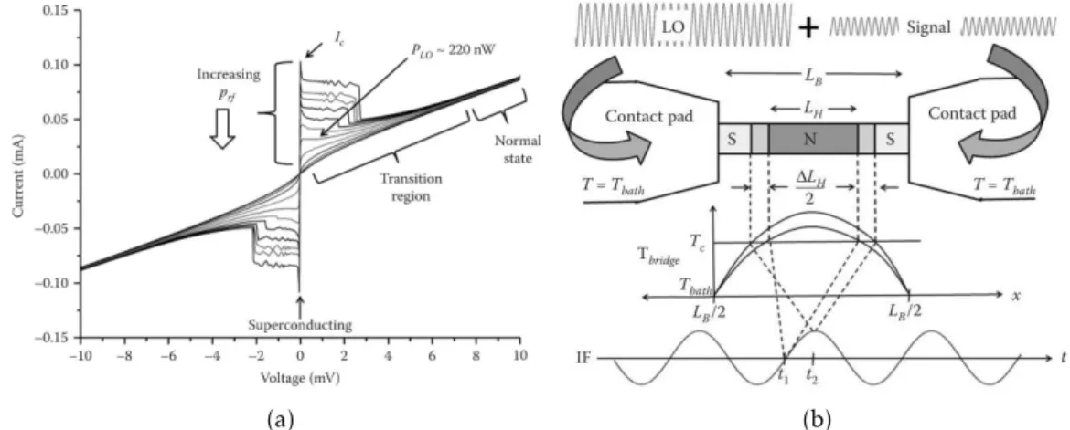
tempera-tures for heterodyne mixers. The curves for 2, 10 and 50 times the quantum noise limit can be seen. From [9] . . . 3 1.3 Ideal HEB IV curves for different pumping powers. b)Hot-spot model of HEB mixing.

The LO and signal power are transmitted through contact pads to either end of the superconductive bridge. The bridge which is biased in order to create a hotspot where the bridge becomes normal, which size is modulated by the combination of incoming signal and LO. From [9] . . . 4 1.4 (a) Surface topology of one unit cell of a Fourier phase grating for 2x2 beams at

1.4THz. (b) 3D profile of the cell in (a).(c) Measurement at 17 cm from the grating. From [24, 25] . . . 6

2.2 a) Device NV08_A2_B results. b) Y factor at 0.9 mV. c) Noise vs bias voltage. . . 11 2.3 Histogram representation of the measurements. a) Normal resistance. b) Critical

current. c) Noise temperature. d)Optimal pumping power. . . 13

3.1 Diagram of the lens design. . . 15 3.2 I-V curves obtained for the different lens. a) umpumped curves. b) Optimal pumped

curves. . . 16 3.3 DSBTrecfor device NV08_B5_A using different lens. Data for 3 µm thickness

beam-splitter. . . 16 3.4 Simulated curves of the lens effi_{ciency vs the extension length. . . . 17}

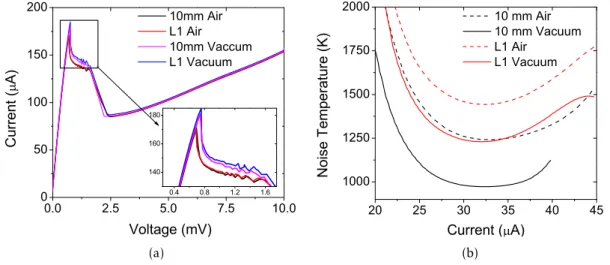
3.5 Air setup . . . 18 3.6 Air vs Vaccum setup results. a)I-V curves. b) Noise curves at the optimum voltage.

The minimums are: 1443 K - L1 Air; 1242 K - 10 mm Vacuum; 1230 K - L1 Vacuum; 973 K - 10 mm Air. . . 18

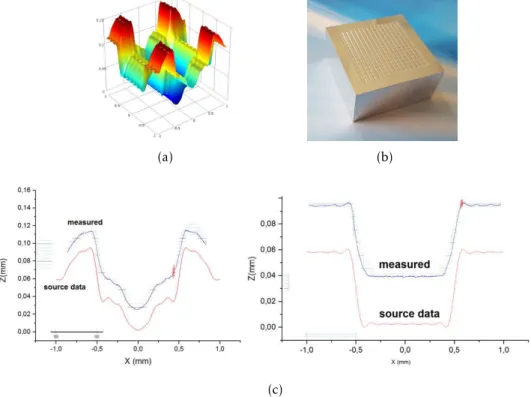
4.1 Fourier phase grating. a)Simulation of one unit cell. b) Fabricated grating (machined surface: 3 cm x 3 cm). c) Profile comparison between measured (real) and source (designed) data. Note: Z offset added to improve visualization of the results, it’s not

a real diff_{erence. . . . . 21}

4.2 Scheme of the experimental setup for the Fourier Phase Grating characterization. . 22 4.4 a) Calibration curve of the data . . . 24 4.5 a) Raw data measured at 25º. b)Correspondent laser values measured as reference. 24 4.6 Beam pattern at 60 mm from the grating at 25 Degrees. a) Direct Imaging. b) Origin

contour plot. c) Direct image after noise removing algorithm. . . 25 4.8 Simulated beam pattern based on the designed surface and perfect collimated

gaus-sian beam. a) 15º. b) 20º. c) 25º. . . 27

L i s t o f F i g u r e s

4.9 3D simulation of the grating beam pattern. a) Flat plan intersection. Representation of the side angles. b) Spherical plane intersection. . . 28 4.11 2x2 HEB mixer array block. a) Front view. b)Back view. Its possible to see the small

HEB chips glued in the center of the lens. c) Array block mounted on the cryostat and connected. . . 30 4.12 a) Highlight of the central beams for the pattern obtained atθ= 25º. b) LO Optical

path scheme for array pumping. This represents the side view of the optical path, with the full pattern being collimated. . . 31 4.14 Picture of the setup used to pump the array during the grating test. The laser beam

comes out of the FIR Gas laser passing through the aperture stop, where the desired beam size is obtained. The beam then illuminates the grating, having the output pattern gathered at the lens. This lens is positioned at a distance (50mm) which match its own f number, allowing to collimate the pattern of the central four beams. The beamsplitter (12 µm thickness, reflects 10% of the radiation from the lens into the cryostat, and simulates where the combination with the astronomical signal will occur. . . 33 4.15 Array umpumped IV curves. . . 34 4.16 Array fully pumped IV curves. . . 35 4.17 Conditions required to collimate the beam pattern and match it to the array used.

a)LensF# vs focal length. b) Lens diameter vs the focal length. . . 36

B.1 Illustration of the GUSTO balloon. . . 45

D.1 3D simulation of the grating beam pattern. Flat plan intersection. Representation of the side angles. . . 49 D.2 Ideal beam pattern. Representation of the different distances considered. . . 49

List of Tables

2.1 HEB and lens characterization setup losses. . . 9

2.2 Comparison between device A and B of the same chip (NV08_A2) . . . 12

2.3 Summary of all the parameters obtained in the characterization of the ten devices studied from batch NV08. . . 12

3.1 Parameters of fabrication for the lens used.εSi represents the dielectric value as-sumed for the optimization of each lens. . . 15

3.2 Minimum noise and optimum bias conditions for the curves in figure 3.3 . . . 16

3.3 Extension length without the substrate thickness for the optical measurement. It also shows the distance from optimum extension, simulated in PILRAP . . . 17

4.1 Efficiency values for both simulated and measured results. . . 28

A.1 Summary of the state of the art on heterodyne instruments . . . 43

C.1 Summary of the instruments used in the entire work. . . 47

Symbols

υ Frequency

υI F IF frequency

υLO LO frequency

εSi Silicon dielectric constant, 11.7 at 300 K

υs Signal frequency

λth Healing distance

F# Lens focal ratio

I_c Critical current

Popt Optimal pumping power

RN Normal resistance

T_C Critical temperature

Tn Noise temperature

Trec Receiver noise temperature

h Planck constant, 6.62607004×10−34_m2_kg/s

kB Boltzmann constant, 1.38064852×10−23m2kg/s2K

[CII] Ionized Carbon

[NII] Ionized Nitrogen

[OI] Neutral Oxygen

NbN Niobium Nitride

Acronymns

LN₂ liquid nitrogen

AR anti-reflective

CPW co-planar waveguide

DSB double sideband

FFT fast Fourier transform

FIR far infrared

GREAT German receiver for Astronomy at Terahertz

GUSTO Galactic/X-galactic Ultra long duration ballon Spectroscopic Stratospheric

THz Observatory

HDPE high density poly ethylene

HEB Hot Electron bolometer

IF intermediate frequency

KID Kinetic inductance Detector

LHe liquid helium

LNA low noise amplifier

LO Local Oscillator

QCL quantum cascade laser

RF radio frequency

SIS Superconductor-Insulator-Superconductor

SSB single sideband

STO Stratospheric Terahertz Observatory

TES Transition Edge Sensor

AC R O N Y M N S

THz Terahertz

Objective

Terahertz radiation is one of the less studied regions of the electromagnetic spectrum, but contains a significant source of information about the cycle of matter in the universe, hence it is crucial for our understanding of how stars with planetary systems came to be. This thesis work is concerned with the viability of developing multipixel heterodyne mixer arrays at super-THz, as a step forward the desired 4.7 THz HEB mixer array for the NASA candidate GUSTO mission, aiming to:

• show that fabrication of detectors (yield) and consistency in performance is sufficiently

good that suffi_{cient HEBs can be drawn from the same batch to populate multipixel arrays.}

• study how the operation of HEBs is affected by the use of different sized elliptical SI lens

in order to achieve smaller dimension array footprint.

• demonstrate capability of dividing a THz beam into 8 at 1.4THz, as a step towards an 8 pixel 4.7 THz receiver for astronomical observations, i.e, GUSTO.

• make suggestions that improve the understanding of gratings and applications of gratings. Transition from 1.4 THz to 4.7 THz is then much more straightforward thanks to this work.

Work structure

To make it easier to understand this work was organized as follows: The motivation intro-duces the importance of astrophysics missions and in special, the mission where this thesis is included, GUSTO; It is followed by the introduction where it is explained the basics on THz astronomy, detection methods, hot electron bolometers, (being this the crucial sensors for THz detection), the state of the art, and finally the Fourier Phase phase grating, which is the key element for the LO multiplexing. Chapter 2, 3 and 4 describe each of the studies made. Chapter 2 includes all the work done on HEB characterization, introducing first the experimental setup used, and later the results obtained. It includes the characterization and sensor selection pro-cess. Chapter 3 introduces the study on lens size vs noise temperature. Here no experimental part is introduced since it’s the same as the previous chapter, and therefore only the results of the experiments and simulation are presented. Chapter 4 summarizes all the work done on the Fourier Phase Grating and represents the core of the work of in this thesis. All the optical path designs are presented for the grating characterization and use, it is also described how the data acquisition and treatment was performed. This is followed by the results chapter and the chapter that ends with the demonstration of a 2x2 receiver array. There are also four appendixes added: the first to introduce with more detail the state of the art on this instrumentation field, the second with detailed presentation to the GUSTO mission, a third with the list of all the instruments used in this work and a fourth with full demonstration of the grating equations that can be used in an array design

Motivation

W

here do we come from?

Since antiquity, human curiosity has been sparked by the stars and planets in the night sky, fueling imagination and creating myths. The recordings of sky observations can be traced as far back as the early man’s drawings in caves and have since then played an important role in humanity, used to predict future events or as adoration idols. In the last centuries by the hand of big names like Newton, Galileu or Kepler, astronomy saw advances with the invention of telescopes leading to the discovery of far away stars, planets and galaxies. More recently, the race to get space probes into space was another mark in astronomy, allowing for telescopes (such as Hubble) and interplanetary probes to extend even further our ability to explore the space. And all of these eff_{orts with a single quest in mind: to find how we came to be.}

Many different missions have been launched in past decades, from stratospheric balloons to

satellites. These have allowed Humanity to start unraveling the mysteries behind the cosmos. The GUSTO mission has an ambitious goal of unlocking for the first time a specific line of THz radiation, [OI] at 4.7 THz, that together with the information of other lines already studied, such as [NII] (1.4 THz) and [CII](1.9 THz), can help trace these molecules and therefore allow us to tap into the life cycle of the interstellar clouds, and possible lead us to an understand, for example, of how systems comprised of stars with planets are formed.

C h a p t e r

1

Introduction

1.1 Terahertz Astronomy

Despite all the advances made in astronomy, there are still some regions of the electromagnetic spectrum that remain largely unexplored. One of these regions is the Terahertz (THz), also known as sub-millimeter or far-infrared radiation, defined as a frequency range between 0.3-10 THz (or 30 µm-1 mm wavelength). This region plays a major role in astrophysics since it is the primary source of radiation for the most luminous spectral signatures of ions, atoms and molecules that permeate the Universe. Although the radiation from, e.g. stars, originates mainly in the visible and ultraviolet part of the spectrum, as this radiation interacts with dust in interstellar clouds, it shifts in frequency by reemission in THz or redshift THz emission. Studying this frequency range enables the study of the evolution cycles of matter in galaxies such as the universe carbon cycle (see figure B.1), the life cycle of the Interstellar Medium and also understanding astrophysical phenomena such as cometary atmospheres. All of this leads to understand how the formation of a star with a planetary system happen.[1, 2]

Figure 1.1: Life cycle of interstellar clouds. The cycle starts from the warm neutral and ionized gas formed in hydrogen clouds. It originates molecular clouds that give rise to stars. The stars evolve and by exploding end up again as ionized gas. At each stage we have

diff_{erent molecules (e.g. [CII]) which study}

can help track this cycle. Adapted from [1]

This understanding can be achieved by measuring conditions such as temperature, pressure and dynam-ics of clouds in galaxies. Temperature and pressure can be obtained with low resolution spectroscopy (co-herent detectors), while for dynamic processes, higher spectral resolution provided by heterodynes (indirect detectors) is more favorable. The astronomical appli-cation of heterodyne is to use the Doppler shift of a known frequency molecular line to calculate velocity, which require high spectral resolution. The more reli-able way to get this data is by studying the Milky Way, where better quality measurements can be performed since other galaxies are too far away to get sufficient

spatial resolutions. The data gathered can be used as a template for other galaxies.

Diffi_{culties with development of THz}

sources/de-tectors and the loss of radiation by absorption from the Earth’s atmosphere (mainly due to water vapour), are

the key aspects hindering the exploration of this part of the spectrum. Thanks to advancements made in superconducting and quantum technology, it was possible to develop and improve single THz receiver which will be discussed later. Since the sensitivity is finite, it is preferable to make use of the brightest molecular frequency lines available, hence the choice of specific lines to be studied such as, the [NII] (1.4 THz), [CII] (1.9 THz) or [OI] (4.7 THz), being the last hardly studied due to existing technology limitations.

C H A P T E R 1 . I N T R O D U C T I O N

1.2 Detection methods

Detection technologies can be simply divided into two categories: incoherent (direct) or coher-ent (heterodyne) detection. Despite direct detectors providing superior sensitivities, they are not suited for applications that require ultra-high spectral resolution, which is key to avoid line blending and resolve line shapes of radiation in astronomy. Due to this, heterodyne re-ceivers are generally used for spectroscopy and direct detectors for imaging or low resolution spectroscopy. [3]

1.2.1 Incoherent detection technology

Direct detectors work simply as power detectors, preserving only the signal amplitude infor-mation. These type of detectors are considered as broadband detetors. Direct detectors couple all the power received within their sensitive band, they therefore require a band-pass filter or spectrometer at the input in order to avoid undesired frequency detection.[3, 4] Example of direct detectors are the Transition Edge Sensor (TES)[5] and the Kinetic inductance Detector (KID)[6].

1.2.2 Coherent detection technology

In heterodyne detection a mixer is used to down convert a signal at THz into an intermediate fre-quency (IF), usually around the GHz (υI F≪υs), while preserving both the phase and amplitude

information of the original signal. This process (see figure 1.2a) starts by taking an unknown signal and combining it optically with an Local Oscillator (LO) using a beamsplitter/combiner, coupling the combined signal with an antenna/waveguide into the mixer. The mixer will only sense the beat of the optical signal coupled, converting it into an eletrical IF as its output, which accordingly to the mixer theory is known to be:υI F=|υs−υLO|. This frequency transformation

allows the signal to be processed by regular radio frequency (RF) electronics. The mixer output is then amplified by the IF amplifier chain, filtered and finally retrieved applying a spectrum analyzer. This produces a spectrometer without any moving parts and with high sensitivity, high spectral resolutions (υ /△υ≥107), but with limited bandwidth. [3]. In the chapter 2 a

detailed description of our heterodyne system can be found.

The LO is required to be a signal with an extremely stable phase or frequency that gives the mixer the "tone" with which to mix the target signal and should have enough power to pump the mixer to its optimum operation point. Until recently the main LO sources used have been the FIR gas laser and Schottky diode frequency multiplier, the former being too big to implement in an instrument, and the later losing power exponentially with frequency hence it has only been demonstrated up to 2.7 THz. More recently an alternative laser technology appeared, the quantum cascade laser (QCL)[7], in which promising power output, frequency range and small size lead to its demonstration as effective LO source at 4.7 THz in 2013 [8]. One of the

downsides of this technology is the use of cryogenic temperatures.

When using a mixer one should take into account the available LO power, operating tem-perature and the sensitivity needed, defined as the noise temtem-perature,Tn, of the receiver. A

mixer can operate in single sideband (SSB) or in double sideband (DSB) mode. The former is defined as when the mixer outputs two diff_{erent IF, one for each of the sidebands, while the}

later only has a single output IF, by which both sidebands are superimposed. The DSB is more

1 . 3 . H O T E L E C T R O N B O LOM E T E R S

typical at THz frequencies due to its simplicity of construction. The noise levels of both modes are related such that:TSSB≈2TDSB. [9]

Due to the use of quantum mechanisms in mixers, both phase and amplitude are non-commuting quantities, therefore, based on the Heisenberg Uncertainty Principle, retaining information of both parts is the reason for the existence of a "quantum limit" for mixer sensitivity. This limit, for SSB operation, can be expressed as a noise temperature, Tn =

hυ

k_B, which is

50K/THz. [9, 10]

(a) (b)

Figure 1.2:(a) Heterodyne detection scheme. (b) Comparison of measured DSB noise temperatures for heterodyne mixers. The curves for 2, 10 and 50 times the quantum noise limit can be seen. From [9]

There are available diff_{erent types of mixer for THz detection such as the}

Superconductor-Insulator-Superconductor (SIS)[11, 12] and the Hot Electron bolometer (HEB) [13, 14], which require cooling to make use of superconducting properties, and the Schottky diodes [15]. Al-though the later uses semiconductor technology and therefore doesn’t have temperature restric-tions, is the one that offers the poorest noise temperature and highest requirement for LO power

(see figure 1.2b). SIS offers the best sensitivies, but as we move for values higher than 1THz

their perfomance deteriorates quickly, hence the HEB being the principal detector at super-THz. [9, 16]

1.3 Hot Electron Bolometers

Hot electron bolometers history starts with Phillips and Jefferts (1973) [13] and later by

Ger-shenzon et al (1990)[14]. These detectors, when used as mixers, are essentially a thin film strip of superconductor material contacted with two normal metal antenna pads. The working principle is the bolometric effect, where small temperature variations due the absorption of

incident photons have a strong impact on the resistance of the sensor, and thus is operated in a resistive state. In figure 1.3a the typical IV curve of an HEB is presented. If no DC bias (VB)

is applied to the device, it behaves as a short, increasing its current until a critical valueIC,

which is the maximum current output, and marks the end of the superconductive zone (ideally this should happen at 0 V, but in real devices this zone can range within a fraction of a mV where we see a low positive resistance behavior due to resistance of the metal contacts). As the voltage increases, Cooper pairs (pairs of electrons) within the bridge start to break leading the device to stop behaving as a pure superconductor, and resulting in a decrease in current (negative resistance behavior). This is called the non-linear transition region. When the voltage magnitude is high enough, it simply behaves as a normal resistance, hence the name for normal

C H A P T E R 1 . I N T R O D U C T I O N

state region. The operation is based on the combination of the DC bias, LO power and a low bath temperature,Tb(using liquid helium (LHe)), such that it sets the device into the non-linear

transition between the superconductive and resistive (normal) state. Since the working princi-ple makes use of hot electrons, from the breaking of cooper pairs, it makes HEB fast enough to act as mixer with reasonable bandwidth. [9]

The mixing in the HEB occurs based on the hot-spot model (see figure 1.3b). When the device is set on the nonlinear transition, the DC dissipation and radiation from the LO heats the bridge creating a zone in the center of the bridge that is in the normal state, referred also as the hot-spot, and has a lengthL_Hin figure 1.3b. Heating due to the absorption of the target signal and LO causesLHto be modulated at a frequency corresponding to the IF, and therefore

the conductivity of the bridge.

(a) (b)

Figure 1.3:Ideal HEB IV curves for diff_{erent pumping powers. b)Hot-spot model of HEB mixing. The LO and}

signal power are transmitted through contact pads to either end of the superconductive bridge. The bridge which is biased in order to create a hotspot where the bridge becomes normal, which size is modulated by the combination of incoming signal and LO. From [9]

The speed at which heat can be driven out of the bridge influences how high the IF band-width can be. The heat transfer mechanism in an HEB can happen both by electrons escaping through the contact pads, or due to electron-phonon coupling to the crystal lattice of the sub-strate. Depending on the distance a hot electron has to travel before losing its energy to the He bath, also called the healing distance (λth), it can be a diffusion cooled HEB[14] whenLb< λth ,

or a phonon-cooled HEB [17], ifL_b> λ_th. The IF bandwidth is the quantity that determines how much of the THz spectrum can be measured (downconverted) at a given time, reaching values as high as 6 GHz, being diffusion-cooled HEB usually the ones providing higher IF bandwidths.

[9, 16]

Another parameter worthy of note in heterodyne instruments is the Allan time. The Allan time is a measure of stability of the system and tells us how long we can be integrating before needing to recalibrate the system. This is a crucial parameter since the stability of an HEB receiver is a complex system due to the need for accurate biasing and optical pumping of the mixer bridge. Typical Allan times for HEB systems can go from 0.1s to around 30s depending on the stability of the system and the noise bandwidth of the measurement.[9]

1 . 4 . H E T E R O DY N E A R R AY I N S T R U M E N T S S TAT E O F T H E A R T

1.4 Heterodyne array instruments State of the art

For practical purposes there is a necessity for having more than one single detector when car-rying out astronomical observations, thus the importance of having arrays of “pixels” (parallel receivers), capable of increasing the mapping speed of the instrument and improve the data quality from measurements.

Currently only a few instruments at terahertz frequencies with limited number of pixels are functional (mainly using SIS mixers or waveguided-based HEB). There is a demand for higher frequency arrays with improved resolution and ability for multiple line spectroscopy, for example STO2 [18], upGreat [19] and the NASA candidate mission GUSTO. The main goal of this last mission is to introduce a state of the art 4x2 pixel array receiver at 4.7 THz and this thesis work aims to take a step closer. A detailed description of the mission can be found in appendix B. The main challenges in developing heterodyne arrays are the LO power multiplexing and injection, the front-end architecture (i.e.,mixers, array configuration, etc), and the circuit components integration. The available LO sources and its multiplexing are by far the main issues since it’s what defines the front-end architecture of the arrays, and whose scarcity is the main reason why there are so few published results at higher frequencies.[20] In the appendix A is a summary of the operational or under development heterodyne array instruments.

1.5 Fourier Phase Grating

When trying to design an array that requires multiple mixers to be pumped at the same time, it would be non-practical in terms of complexity and tunability to use a single LO source for each of the pixels. To solve this problem researchers came up a number of solutions such as Dammann gratings or wave guide couplers[21], but the problem still lingers due to the lack of flexibility, frequency limitations, or difficulties in fabrication. The Fourier phase gratings

introduced by Murphy et al(1999) and Graf et al(2001) [22, 23] is an elegant solution for this problem, allowing flexibility to the system due to a continuous phase modulation of light and easy direct milling fabrication methods. This element is crucial when dealing with multipixel QCL pumped arrays, since multi QCL implementation would be too complex to design due to this devices high thermal dissipation, requiring huge amounts of cryogenic liquids/reservoirs, and need for perfect frequency locking.

The Fourier phase grating, a reflective grating, allows user to engineer a diffraction pattern

to any shape, dividing equally a single coherent incident beam into multiple sub-beams. This is possible due to the use of periodic smooth structures (cells) on its surface designed based on the Fourier series expansion theory. It uses phase manipulation of the terahertz waves in such a way that the multiple sub-beams are formed in the far field. The spatial phase modulation of a 1-D Fourier grating can be obtained by the Fourier series expansion [23]:

△ϕ(x) =

N

X

n=1

ancos

n

2_πx

D

(1.1)

Being the unit cell defined as−D 2 ≤x <

D

2 and whereanare the key parameters that determine

C H A P T E R 1 . I N T R O D U C T I O N

the grating surface structure. ForN= 1 the far-field of this phase grating becomes:

U(θ) =U0

∞

X

q=−∞

Jq(a)δ

θ−qλ D

(1.2)

HereJ_q(.) denotes the Bessel function of the first kind of order q. ForN >1 the modulation at the grating plane can be written as:

U0ej△ϕ(x)=U0

N

Y

n=1

e

jancos

     n       2πx D             (1.3)

Which is nothing more than the product of the fields modulated by the individual fourier components, i.e, the Fourier transform of the grating. Finally, the far-field diffraction pattern

of this field is obtained by the multiple convolutions of the diff_{raction fields of the individual}

Fourier components:

U(θ) =U0× ⊗Nn=1

       ∞ X

q=−∞

J_q(a_n)δ

θ−qnλ D        (1.4)

Although equation 1.4 best define our grating, the fastest way to obtain the structure is to run a fast Fourier transform (FFT) algorithm to directly calculate the Fourier transform of the grating (equation 1.3), optimizing the a_n coefficients that best generate the desired far-field

pattern (i.e, reflected beam pattern). More details on how to obtain the structure can be found in [23].

(a) (b) (c)

Figure 1.4:(a) Surface topology of one unit cell of a Fourier phase grating for 2x2 beams at 1.4THz. (b) 3D profile of the cell in (a).(c) Measurement at 17 cm from the grating. From [24, 25]

The advantages that this type of grating brings to the astronomy field is that it allows for a large number of beams to be obtained from a single source of LO, hence greatly simplifying array systems and solving the issue of the scarcity of LO sources. Furthermore, due to the dimension of THz wavelengths, this type of grating can be simply milled on a surface, without the need for highly complex lithographic systems. So far the highest frequency for which a grating was demonstrated to be an eff_{ective LO multiplexer was at 1.4THz with a 2x2 beam}

pattern by the works of both Y.C. Luo and X.X. Liu [24–27].

For array applications, the key parameter of the grating, besides obviously the beam pattern, is the angular distribution of the emergent beams, which depends on the unit cell size, working wavelength and order mode.

C h a p t e r

2

HEB characterization: 4x2 pixel array assembly

Future requirements for GUSTO will require many HEB mixers with similar performance. Part of the work here is a study of mixer performance within a fabrication batch to check the variation in sensitivity, pump power and superconductingIc. Identified mixers are part of flight

hardware selection, making the testing critical to avoid loss of devices.

It will be presented the experimental setup to characterize the HEB that will be followed by the results obtained. The setup used to characterize the HEB is the same used in the lens study in chapter 3.

2.1 HEB and Si Lens characterization setup

As explained in section 1.3, working with the HEB requires a complex setup in order to maintain the balance between key parameters such as the temperature of the bath, bias voltage, etc. The setup used in this work is summarized in the scheme found in figure 2.1a. Using our setup it is possible to bias the mixer and obtain its I-V curve, where theIccan be extracted, and the IF

output which is used to calculate the noise temperature using the Hot/Cold Y factor technique (see section 2.1.1) with the help of a hot and cold load.

The key element of our setup is the cryostat where the mixer and all the circuitry required to operate it are placed. In the cryostat we have different shields to enable the use of cryogenic

temperatures: the outer vacuum shield, an intermediate shield using liquid nitrogen (LN₂) at 77

K, and the inner shield, for LHe at 4 K. The last one is the most critical since is connected to the mixer block and circuitry, working as the heat sink responsible for maintaining the temperature at around 4 K, which is below theT_C of the HEB’s. Connected to the cryostat we have an arm equipped with two black bodies (see figure 2.1a): one of them in direct contact withLN2hence

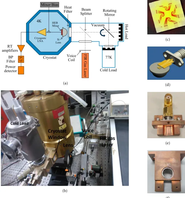
working as a cold load, and the second black body, at room temperature, working as a relative hot load. A rotating mirror is used to change between loads. The well known signal is then oriented into a beamsplitter where it is combined with the LO signal coming from a far infrared (FIR) gas laser, redirecting the combination into the cryostat. The combined signal passes a heat filter which works as a low pass filter, allowing only radiation below 6 THz to pass through. After passing the heat filter the radiation is then collected by an elliptical Si lens focusing the radiation into the HEB antenna after which it is coupled into the HEB. The optical beat frequency is converted into electrical IF by the mixer. After the IF signal is extracted from the HEB, it is amplified in a cryogenic low noise amplifier (LNA). Outside the cryostat the signal is further processed by the IF warm chain, which is comprised of room temperature amplifiers, a bandpass filter, and a power detector. In appendix C the list of the instruments used for all the experiments (including grating characterization) can be found.

In figure 2.1c we have an example of the HEB chips used. All the devices characterized were produced at TUDelft. Each chip used has four spiral antennas/HEB’s, referenced from A to D. Each HEB was fabricated using NbN as the superconductor material for the bridge. The width for all bridges was 2 µm and the length 0.150(A), 0.200(B), 0.200 (C), 0.250 (D) µm. The option for spiral antenna comes from the broad spectrum coverage it allows, since a single device can this way be operated between 1 and 6 THz.

C H A P T E R 2 . H E B C H A R AC T E R I Z AT I O N : 4 X 2 P I X E L A R R AY A S S E M B LY H o t L o ad Cold Load Cryogenic LNA HEB Mixer Cryostat Si Lens 77K 4K Vacuum F IR G as L as er Voice Coil Mixer Bias Rotating Mirror RT amplifiers BP Filter Power detector Heat Filter Beam Splitter (a) (b) (c) (d) (e) (f)

Figure 2.1:a)HEB and Si lens characterization scheme. b)Experimental setup. The lens presented can be used or not, to facilitate the radiation coupling into the cryostat. c)Example of a HEB chip used. Four spiral antenna HEB are present. d) CAD 3D scheme of the HEB mounted on the Si lens and IF/bias CPW circuitry. e) CPW circuit used. f) 10 mm lens holder used.

In figure 2.1d one can see the CAD model on how each chip is mounted on the Si lens, and how the IF/bias circuitry is connected to the HEB. For this circuitry a co-planar waveguide (CPW) is used to transmit the signals. The HEB is glued onto the lens, using a combination of an optical microscope with a micrometer XY stage to achieve alignment accuracy in the order of 1 µm. The focal point of the SI lens used is located in it’s geometrical surface center at a height equal to the chip thickness. After having the chip on the lens, the mixer block is added, wire bonding the contacts of the desired HEB, with the mixer block circuit. The mixer block is then placed on the cryostat, wired to the IF chain and bias supply, followed by closing it. Vacuum levels (10−5 _{mbar) are then achieved using a two stage vacuum pump, followed by cooling,}

2 . 2 . R E S U LT S

firstly usingLN2and later by LHe.

This setup is what we define as vacuum setup since the hot/cold signal remains in vacuum, where the best conditions for measurement are possible. Sometimes however, for greater flex-ibility or in the case of an array test, the vacuum setup is removed and hot/cold signal and beamsplitter are placed in air, in this case it is referred as air setup.

The FIR gas Laser works as our LO since its frequency can be easily tuned accordingly with our needs (in this work different frequencies were used, which will be addressed in the results).

2.1.1 Hot/Cold Y factor Technique

The hot/cold Y-factor technique based on the Callen & Welton noise temperature descrip-tion[28] is a method that allows calculation of the noise temperature of a mixer system from its measured Y factor.

By coupling two difference noise sources (an hot and a cold load), one at a time, and

mea-suring the output IF power of the receiver, it’s possible to derive theTn:

Tn=

Thotload−Y Tcoldload

Y−1 (2.1)

where

Y = Photload

Pcoldload

(2.2)

P_hotload andP_coldload are the the output power of the receiver for each of the loads used,

obtained using the Callen and Welton description of noise temperature converted to power[28]:

PCW=

hυ e        hυ kT        −1 +hυ 2 (2.3)

TheTn calculated this way will take into account all the losses in the setup due to the use

of optic elements (see table 2.1), therefore it is referred as the receiver noise, DSBTREC. By

considering these losses it is possible to obtain the noise temperature of the HEB mixer itself as done in the work of Zhang et al [29].

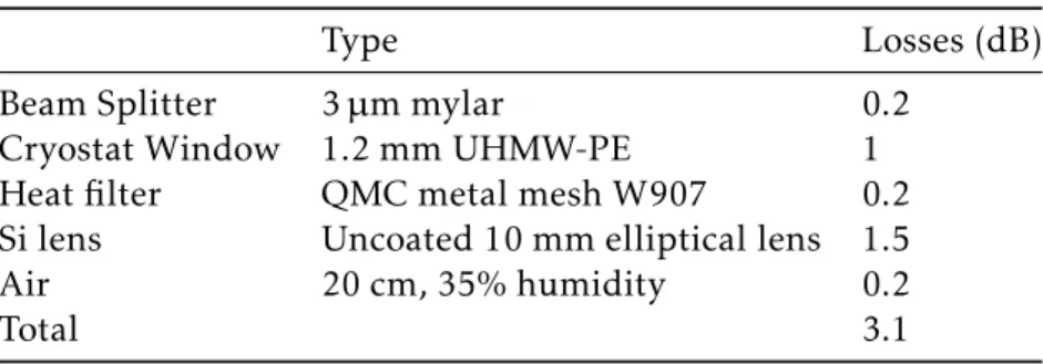
Table 2.1:HEB and lens characterization setup losses.

Type Losses (dB)

Beam Splitter 3 µm mylar 0.2

Cryostat Window 1.2 mm UHMW-PE 1

Heat filter QMC metal mesh W907 0.2

Si lens Uncoated 10 mm elliptical lens 1.5

Air 20 cm, 35% humidity 0.2

Total 3.1

2.2 Results

After some preliminary studies with diff_{erent devices from various fabrication batches}

pro-duced by TUDelft, it was decided to study devices from a single batch, all from the same wafer defined asNV08. The goal here was to obtain at least 8 devices with similar properties. Only the results of this process are discussed since the preliminary tests were used with the idea of getting some experience dealing with all the process.

C H A P T E R 2 . H E B C H A R AC T E R I Z AT I O N : 4 X 2 P I X E L A R R AY A S S E M B LY

Although the target frequency is 4.7 THz, direct characterization at such a frequency would not be practical. With our FIR gas laser, it’s not been possible to get a 4.7 THz line working, so it would require the use of a QCL, of which only one was available and there was some risk off_{destroying it due to improper operation (due to lack of experience of my part). Moreover}

it would require another cryostat, more liquid helium, which all together would take much longer to setup and would turn the experiences much more expensive. Therefore, and since for GUSTO there is also the requirement for a 1.4 and 1.9 THz array, it was decided to use the FIR gas laser tuned to 2.5 THz. This frequency was chosen because was one of the easiest to work with, with enough power to pump virtually any device (within the expected pumping power). For the characterization, only theTnis frequency dependent, and based on previous studies is

possible to extrapolate what this value its equivalent at 4.7 THz.[29]

2.2.1 In-chip device selection

When starting to study batch NV08 it was decided to begin by getting an idea of the best in chip HEB’s characteristics, and then move into studying the same reference on the others chips. From the first chip, NV08_A2 we started by studyingdevice B, since the bridge length is in between the other options. The results for this device can be seen in figure 2.2.

The key parameters studied were: the normal resistance (RN), measured directly; the I-V

curve, from where theIC is extracted; the noise temperature (Tnor DSBTrec); and the optimal

pumping power (Popt). The first thing to analyze is the umpumped I-V curve of the HEB which

is measured when no LO is applied. Device NV08_A2_B can be seen in figure 2.2a, from which we can easily extract theIC of the device.

Secondly it is needed to understand what are the noise characteristics for different bias

voltages, with the final goal of finding the optimum bias conditions (i.e. where the lowest noise is measured). In order to accomplish this, different Y factor measurements are performed at

several bias voltages. At each one, the following steps were taken: 1. guarantee the LO power was enough to fully pump the device (the more resistance like I-V curve the best); 2. Apply the wanted bias voltage and select the first load (Hot or Cold); with the help of an in-house Labview program, scan between two current values with a set step (usually from 20 µA to 45 µA, with steps of 1 µA), measuring the output IF power. The current variation is achieved thanks to the use of the PID control on the voice-coil, that blocks the amount of LO power reaching the HEB, inducing an increase on the current; 3. Repeat step 2 with the complementary load; 4. Using another Labview program, the minimum noise temperature is obtained based on the Y factor of the measurements in 2 and 3. For this, the data is fitted into a polynomial function , which is then used to calculate the Y factor, finally converting the Y-factor into noise temperature, where the minimum is extracted; 5. Repeat steps 2-4, until a total of 3 noise measurements were made. Figure 2.2b shows theTn values measured this way for different voltages. The center

point plotted is the average value measured, and the error bars represent the standard deviation. Knowing how the noise behaves allows us to pinpoint what the best operation voltage should be. In this case both 0.8 mV and 1 mV show the lowest values among the voltages studied, so both were measured again but using a smaller current step ( 0.25 µA instead of 1 µA), in order to obtain more reliable measurements. Here theTnobtained was of 906 K at 0.8 mV and 911 K

2 . 2 . R E S U LT S

at 1 mV. Since both were so close, 0.9 mV was also measured yielding 903 K minimum noise, at 37 µA as seen in figure 2.2c.

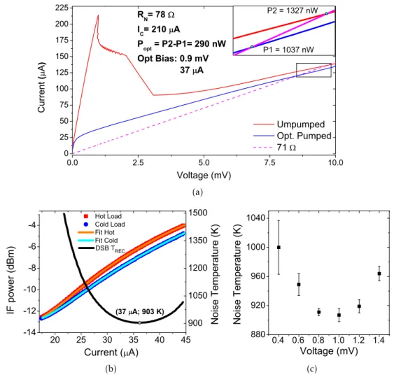
0.0 2.5 5.0 7.5 10.0 0 25 50 75 100 125 150 175 200 225 C u r r e n t ( A ) Voltage (mV) Umpumped Opt. Pumped 71 R N = 78 I C

= 210 A

P

opt

= P2-P1= 290 nW Opt Bias: 0.9 mV

37 A

P1 = 1037 nW P2 = 1327 nW

(a)

20 25 30 35 40 45 -14 -12 -10 -8 -6 -4 I F p o w e r ( d B m )

Current ( A)

Hot Load Cold Load Fit Hot Fit Cold 900 1050 1200 1350 1500 DSB T REC N o i s e T e m p e r a t u r e ( K )

(37 A; 903 K)

(b)

0.4 0.6 0.8 1.0 1.2 1.4 880 920 960 1000 1040 N o i s e T e m p e r a t u r e ( K ) Voltage (mV) (c)

Figure 2.2:a) Device NV08_A2_B results. b) Y factor at 0.9 mV. c) Noise vs bias voltage.

For last it was measured the optimal pumping power (Popt). Its calculation is based on the

isothermal method [30], where a resistance line is used to interpolate both umpumped and optimum pump IV curves in the normal region. The pumping power is obtained by calculating the difference of power between both interpolation points. The optimum I-V curve is obtained

by biasing the HEB with the optimum voltage, and block the LO beam in such way that the measured current is also the optimum, then a voltage sweep is performed leading to the desired I-V curve. The calculation based on this method can be seen in figure 2.2a, in this case thePopt

was 290 nW.

It is expected to see an increase of about 30% in the noise from 2.5 to 4.7 THz, but since the final lens will use an anti-reflective (AR) coating, reducing the total noise by about the same amount, we can assume the values measured for uncoated lens at 2.5 THz will be roughly the same as the final values at 4.7 THz with the coated lens. Therefore, the noise values for this device are within the required specifications for GUSTO, where we are looking for final sensitivities below 1500 K. The only problem is the pumping power, which is high. In order to bring down this value,device Aof the same chip was also studied following exactly the same methods. Table 2.2.1 summarizes the data measured for both HEB A and B on chip NV08_A2.

C H A P T E R 2 . H E B C H A R AC T E R I Z AT I O N : 4 X 2 P I X E L A R R AY A S S E M B LY

Table 2.2:Comparison between device A and B of the same chip (NV08_A2)

Device R_n(Ω) _Ic(µA) _DSBTrec(K) _Popt (nW)

NV08_A2_B 77 210 903 289

NV08_A2_A 60 270 962 247

Although device A shows higher noise values, these are within the requirements for GUSTO, but the LO power required is about 15% lower, which will help in the use of the QCL + grating. It was decided to move forward studying all the A devices in the chips available.

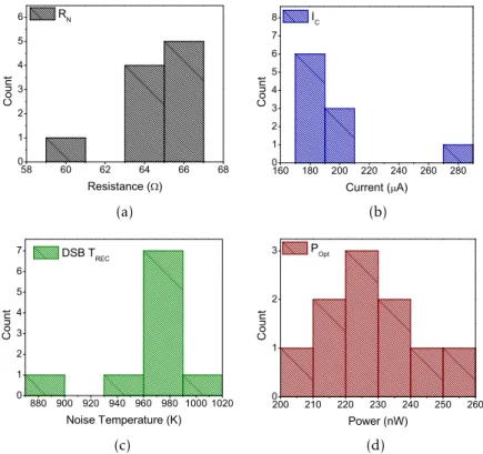
2.2.2 HEB characterization from batch NV08

In total 10 different devices were studied. All of their data is summarized in table 2.3, the

distribution of the various parameters can also be seen in figure 2.3. From those results its clearly that all devices are working and are within the specifications for noise (average 962K) and based on the average LO power required (227 nW) it will all depend on the combination QCL + grating.It should also be noted that the flatness seen in the noise temperature for device NV08_A2_B (see figure 2.2c), is present in all the devices studied, so it is possible to vary the pump power used (within an acceptable range) with little variation on the noise temperature. Furthermore, there is a clear low dispersion of values within all of the parameters, being the critical parameters standard deviation of 29 K (3%) for the noise temperature and 13 nW (6%) for the LO pumping power which might translate into a very uniform array. All of this combined indicates that more devices can be draw from this batch if such necessity arise.

NV08_A2_A due to its high Ic seems a bit off in this population. Since it was studied

previously in 2013, with time the solder left from the bond wiring might have cause some effect.

For this, we won’t be picking this device for the array. Another HEB, NV08_B5_A, was used for all of the lens study in the following section, and although no performance issues were detected, we would rather not use it either.

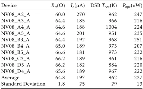
Table 2.3:Summary of all the parameters obtained in the characterization of the ten devices studied from batch NV08.

Device Rn(Ω) Ic(µA) DSBTrec(K) Popt(nW)

NV08_A2_A 60.0 270 962 247

NV08_A3_A 64.4 185 966 216

NV08_A4_A 64.6 188 1004 224

NV08_A5_A 64.6 201 951 235

NV08_B3_A 64.4 192 968 251

NV08_B4_A 65.0 189 973 207

NV08_B5_A 66.6 181 973 232

NV08_C3_A 66.2 189 961 216

NV08_D3_A 66.2 182 884 220

NV08_D4_A 65.6 189 967 222

Average 64.8 197 962 227

Standard Deviation 1.8 25 29 13

2 . 2 . R E S U LT S

58 60 62 64 66 68 0 1 2 3 4 5 6 C o u n t

Resistance ( ) R

N

(a)

160 180 200 220 240 260 280 0 1 2 3 4 5 6 7 8 C o u n t

Current (A) I

C

(b)

880 900 920 940 960 980 10001020 0 1 2 3 4 5 6 7 C o u n t

Noise Temperature (K) DSB T

REC

(c)

200 210 220 230 240 250 260 0 1 2 3 C o u n t Power (nW) P Opt (d)

Figure 2.3:Histogram representation of the measurements. a) Normal resistance. b) Critical current. c) Noise temperature. d)Optimal pumping power.

C h a p t e r

3

Lens size vs noise temperature Study

One of the changes to be introduced into GUSTO from previous instruments such as STO-2, is the moving into smaller diameter lens. This will allow for more compact arrays, and therefore smaller optics systems. In order to understand how smaller lens can have an impact in the noise temperature of devices, three different lens were fabricated and then compared with the

lens used in the HEB characterization, which happen to be similar to the ones used in arrays. The goal here was to discover which of the lens design was the best, and at the same time, how much noise increase should be expected. The four lens are labeled as: 10 mm (the standard test lens), L1, L2 and L3. The last three represent diff_{erent designs for a 3.1 mm type lens. All the}

lens have an elliptical shape, following the equationx

a

2 +y

b

2

= 1, being the value of b and the extension length optimized assuming different dielectric constants for the lens. Table 3.1

summarizes the parameters for each lens. b

Extension

lens diameter a

Figure 3.1:Diagram of the lens design.

Table 3.1:Parameters of fabrication for the lens used.εSi

represents the dielectric value assumed for the optimiza-tion of each lens.

Lens a (mm) b (mm) Extension_(mm) εSi

10 mm 5.0 5.228 1.232 11.4

L1 1.550 1.621 0.134 11.7

L2 1.550 1.623 0.141 11.4

L3 1.550 1.624 0.145 11.2

In terms of experiments, the procedure followed exactly the same steps as those used to characterize the HEB’s, but this time the changing parameter was the lens, and it was used the same HEB, device NV08_B5_A.

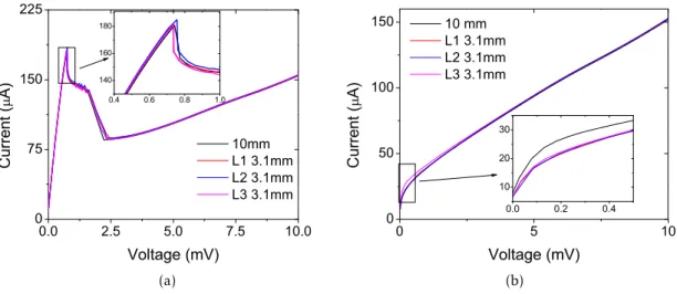
One of the main concerns during the experiments was in guaranteeing that the thermal dissipation in the smaller lens would be the same as in the big one, since they had to be glued to the smaller mixer block used, whereas the normal one simply sits on a indium soft metal ring. Therefore, looking into the results obtained it should firstly be analyzed the I-V curves for the different lens, shown in figure 3.2. In the inset of figure 3.2a, the plot showing unpumped

curves plot (see figure 3.2a) it can be seen with more detail that the curves are overlapping and that theIC values are very close to each other. Since the bridge temperature sets theIc, the

device temperature is verified to be the same using the different lenses, hence the conclusion of

the proper working and similar thermal dissipation of the device throughout the experiments. In the case of the optimum pumped curves (3.2b) it’s also possible to observe the overlapping of the curves, proving the similar operation of the device and therefore allowing for direct comparison of results. There is a small diff_{erence for the umpumped curve of L3, which is}

due to the optimum bias conditions being different than for the rest of the lens. This change

is related to the following results on the noise temperature, and the already expected bad performance of this lens.

C H A P T E R 3 . L E N S S I Z E VS N O I S E T E M P E R AT U R E S T U DY

0.0 2.5 5.0 7.5 10.0 0 75 150 225 C u r r e n t ( A ) Voltage (mV) 10mm L1 3.1mm L2 3.1mm L3 3.1mm

0.4 0.6 0.8 1.0 140

160 180

(a)

0 5 10

0 50 100 150 C u r r e n t ( A ) Voltage (mV) 10 mm L1 3.1mm L2 3.1mm L3 3.1mm

0.0 0.2 0.4 10

20 30

(b)

Figure 3.2:I-V curves obtained for the different lens. a) umpumped curves. b) Optimal pumped curves. In figure 3.3 the Y factor measurements for each lens at the best bias conditions are plotted, while table 3.2 summarizes the minimum for each of the measurements and it’s bias conditions. Early experiments on the noise measurements lead to the use of a 15 µm beamsplitter to pump L1, later solved by using a lens to focus the LO power into the cryostat (used in the experiments of L2 and L3). This lead to no real data being available for the 3 µm beamsplitter for L1. Based on the measurements for the 10 mm lens and L2 where both beamsplitter have been used, it was possible to make the beamsplitter correction from 15 to 3 µm thickness and obtain the curve for L1.

20 25 30 35 40 45 50 1000 1500 2000 2500 N o i se t e m p e r a t u r e ( K )

Current ( A) 10 mm

L1 (BS corrected) L2

L3

Figure 3.3:DSBT_recfor device NV08_B5_A using diff_{erent lens.}

Data for 3 µm thickness beamsplitter.

Table 3.2:Minimum noise and optimum bias conditions for the curves in figure 3.3

Lens V (mV) I (µA) T_n(K)

10 mm 0.6 32 973

L1 0.6 32 1230

L2 0.6 32 1287

L3 0.6 38 1522

Based on the results obtained is clear that there is a similarity between L1 and L2, with L3 being very different, even in the optimum bias conditions. The bad performance for L3 was

already expected since the dielectric value for which it was optimized (11.2) was known to be wrong. The main conclusion here, besides that the design of L1 seems to be the best, is also the increase of approximately 26% in noise between the 10 mm diameter lens and L1, which still sits within the desired noise requirement for GUSTO.

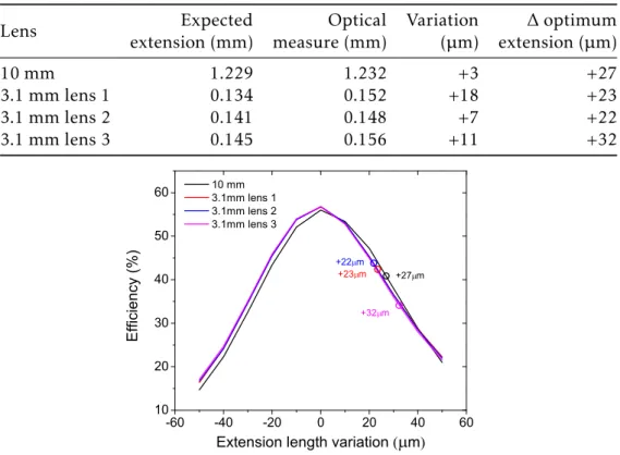
In an attempt to better understand the results obtained, the lens performance was simulated based on the real dimensions measured. This was performed by Ricardo Farinha at TU Delft and more details can be found in his work [31]. Table 3.3 summarizes his measurements results and

comparison with the optimum values obtained through simulations. The simulations assumed the correctεSi at cryogenic temperatures to be 11.4 . Some differences between the measured

parameters and the original design that can highly impact the real efficiency of the lens. This

is clear in figure 3.4 where the lens effi_{ciency vs extension length for all the lens are plotted.}

These results indicate that L1 and L2 should have similar efficiency and therefore similar noise

behavior, which confirms the experimental results. The difference is that L2 was expected to

be the best which is not the case. Since the values obtained via experimental work are very similar, the cause for this difference could be due to noise in the measurements, or a small HEB

misalignment from one measurement to another. A important conclusion that can be drawn is that any small variation on the extension length or the substrate (chip) thickness can have a very high impact on the device performance. This can also be applied to misalignment of HEB when placing them on the lens.

Table 3.3:Extension length without the substrate thickness for the optical measurement. It also shows the distance from optimum extension, simulated in PILRAP

Lens _{extension (mm)}Expected _{measure (mm)}Optical Variation_{(µm) extension (µm)}∆optimum

10 mm 1.229 1.232 +3 +27

3.1 mm lens 1 0.134 0.152 +18 +23

3.1 mm lens 2 0.141 0.148 +7 +22

3.1 mm lens 3 0.145 0.156 +11 +32

-60 -40 -20 0 20 40 60 10

20 30 40 50 60

+32m

+27m

+23m

E

f

f

i

ci

e

n

cy

(

%

)

Extension length variation ( m)

10 m m 3.1m m lens 1 3.1m m lens 2 3.1m m lens 3

+22m

Figure 3.4:Simulated curves of the lens efficiency vs the extension length.

During the experiments a feeling of uncertainty towards our vacuum setup started to build up. The reason for this is that in the vacuum setup, the hot/cold load has a limited size, and since the lens diameter changes there was a chance of this limitation to affect the measurements,

e.g. the misalignment between the loads and lens position inducing error. In the air setup (figure 3.5), the loads are much bigger, which allow to fully cover the cryostat window, hence making sure that any lens within its diameter to receive the maximum radiation possible from both loads. Therefore, to complete the lens characterization it was decided to study the impact of the air vs vacuum setup on the noise measurements.

C H A P T E R 3 . L E N S S I Z E VS N O I S E T E M P E R AT U R E S T U DY

Figure 3.5:Air setup

The results obtained for air vs vacuum setup are plotted in figure 3.6. The first de-tail that should be noticed is the I-V curve dif-ference between the sets of data for air and vacuum measurements. There is a decrease on the IC from the original 181 to 171 µA.

This drop is caused by the larger diameter of the optical components used in this setup, which causes more radiation to be introduced into the cryostat, heating the mixer block and therefore the device, hence this change. In terms of noise measurements there is an inter-esting difference on the increase of noise for

both lens: in the case of the 10 mm lens the

noise increases about 28%, while for L1 the increase is only 17%. It was expected that the change be the same in terms of proportion, and since we have such a difference we conclude

that our hypothesis was right. On one hand both lenses suffer from the same issues from

vac-uum to air: we have loss of the load signal by absorption when passing through the cryostat window, plus the absorption in the optical path by the air humidity (which is expected to be much smaller than the previous noise source, although difficult to quantify), these effects cause

for the signal-to-noise to be reduced. At the same time the loads source are much bigger, so basically it is possible to be sure that no misalignment exists between the lens and the sources, which in the case of the smaller lens, allows it to see all the radiation from the cold load (pos-sibly our problem), and this way, improving the noise temperature which compensates for the negative effects, thus the variation detected being smaller for L1.

0.0 2.5 5.0 7.5 10.0 0 50 100 150 200 C u r r e n t ( A ) Voltage (mV) 10mm Air L1 Air 10mm Vaccum L1 Vacuum

0.4 0.8 1.2 1.6 140

160 180

(a)

20 25 30 35 40 45 1000 1250 1500 1750 2000 N o i se T e m p e r a t u r e ( K )

Current ( A) 10 mm Air 10 mm Vacuum L1 Air

L1 Vacuum

(b)

Figure 3.6:Air vs Vaccum setup results. a)I-V curves. b) Noise curves at the optimum voltage. The minimums are: 1443 K - L1 Air; 1242 K - 10 mm Vacuum; 1230 K - L1 Vacuum; 973 K - 10 mm Air.

Although more experiments are required using improvements to the vacuum setup, it can be concluded that although the noise temperature increases with a smaller lens, it should be anticipated that the increase under vacuum conditions will be below 26%, from the best value

obtained for L1 and concluded to be an overestimation of the real noise. Even assuming this value as the real one, it would set the average noise temperature of the receivers characterized in the previous chapter around 1200 K which is still below the GUSTO requirements, allowing the conclusion that it is possible to move into smaller lens in the future arrays.