Exact Barrier Option Valuation with Deterministic Volatility
†E. ROSALINO Jr.1, A.J. SILVA1, J. BACZYNSKI1* and D. LE ˜AO2
Received on June 27, 2014 / Accepted on January 21, 2015
ABSTRACT.Focus, in the past four decades, has been obtaining closed-form expressions for the no-arbitrage prices and hedges of modified versions of the European options, allowing the dynamic of the underlying assets to have non-constant parameters. In this paper, we obtain a closed-form expression for the price and hedge of an up-and-out European barrier option, assuming that the volatility in the dynamic of the risky asset is an arbitrary deterministic function of time. Setting a constant volatility, the formulas recover the Black and Scholes results, which suggests minimum computational effort. We introduce a novel concept of relative standard deviation for measuring the exposure of the practitioner to risk (enforced by a strategy). The notion that is found in the literature is different and looses the correct physical interpretation. The measure serves aiding the practitioner to adjust the number of rebalances during the option’s lifetime.
Keywords: barrier option, no-arbitrage pricing, hedging, Martingale measure, time-change for Martin-gales.
1 INTRODUCTION
Under arbitrage-free assumptions, Black & Scholes [1] and Merton [17] pioneered the achieve-ments on pricing and hedging derivatives in financial markets. They considered an European call option and a market with one bond and one stock where the parameters in the dynamics that model the market have constant values. By its turn, Harrison & Pliska [4] – among others – showed that, essentially, there is an equivalence between absence of arbitrage opportunities and the existence of an equivalent measure that renders the discounted underlying stock a martin-gale: under this measure, pricing a derivative is allowed to be naively obtained, in that average is applied to the discounted payoff, conditional to the present information.
Underpinned by these seminal results, significative advances followed in obtaining closed-form expressions for the exact prices and hedges of options, as can be verified, for instance, in the
*Corresponding author: Jack Baczynski
†This work was partially supported by CNPq under the Grant No. 472474/2010-0. A preliminary version of this Note
was presented at the Sixth Brazilian Conf. on Stat. Modelling in Insurance and Finance, Maresias/SP, 2013.
1National Laboratory for Scientific Computing – LNCC, Syst. & Contr. Dept., Av. Getulio Vargas, 333, 25651-075 Petr´opolis, RJ, Brasil. E-mails: [email protected]; [email protected]; [email protected]
works of Heston [5] addressing the Ornstein-Uhlembeck format for stochastic volatility, Cox & Ross [2] focusing CEV (constant elasticity of variance) models, and Lo et al. [15] for CEV with deterministic time-dependent coefficients. The case of pure deterministic time-dependent coeffi-cients are direct extensions of [1] (see, e.g., [12]). But the results and techniques do not replicate if entering with more sophisticated derivatives as path dependent options, particularly barrier options. Indeed, achievements in terms of closed-form pricing formulas are more restricted in this case.
Barrier options are standard European options which involve a barrier constraint tailored for a certain behavior of the underlying asset along the option’s lifetime. If this behavior is what the investor thinks will happen, then he may pay less buying the barrier option instead of its standard counterpart (the European option), obtaining the same result whenever his beliefs meet reality. Otherwise the option’s payoff cancels (see, e.g., [3, 12]). Barrier options have been present for more than two decades in the foreign exchange, equity and commodity markets and became very popular in recent years.
Merton [17] derived a closed-form solution for the price of a down-and-out European call option with constant barrier. Explicit solutions for arbitrage-free prices of some other types of barrier options are found in the work of Rubinstein & Reiner [20]. Rich [18] derived closed-form solu-tions for European barrier opsolu-tions with a fixed rebate and constant barrier, as well as exponential barriers with constant time coefficient on the exponent. Heynen & Kat [6, 7] derived closed-form pricing formulas for partial barrier options, and analytic valuation formulas for outside barrier options as well. Via a modified version of the method of images, Kwok et al. [11] extended this scope allowing more than one underlying asset and barriers that can be constant or expo-nential with a constant time coefficient. Kolkiewicz [9] addressed several types of double-barrier options where an infinite series representation for the price is given. Relying on the hitting prob-abilities of a Brownian motion technique, closed-form expressions for European style double barrier options are also encountered in [16]. Using probabilistic techniques, Kunitomo & Ikeda [10] evaluated options contracts monitored by two knock-out barriers with exponential format, whose valuation formulas are given in terms of an infinite series representation. The works above assume that the market model has constant parameters. Allowing the parameters in the dynamics to be deterministic functions of time, Roberts & Shortland [19] explicitly derived approximation formulas for the prices of barrier options by means of estimating the boundary crossing times of the asset price and the technique of hazard rate tangent approximations. Lo et al. [13], via the method of images, obtained estimates of prices of barrier options with generic (square integrable) trajectories. The estimates stem from a parameterized class of trajectories which spontaneously arises from the technique and for which the prices are exact. Considering the CEV models with time-dependent coefficients, Lo et al. [14] also obtained estimates for the prices of barrier op-tions with generic trajectories, brought out by a parameterized class of trajectories for which the prices are exact.
In this note, we present closed-form expressions for the exact price and hedging strategy of an up-and-out call option with a constant barrierB. The barrier tests whether the priceS(u)of the risky asset – which evolves according to the stochastic differential equation
– agrees withS(u)≤ B ∀u ∈ [0,T]. In the above expression the mean rate of return (drift)µ and the volatilityσ are arbitrary deterministic functions of time subject to the mild constraint of square integrability (jumps are allowed, for instance).W is a standard Brownian Motion andT is the expiration time. We assume the riskless interest rater =0.
We justify modeling the market via a deterministic time dependent volatility noticing the fol-lowing. Market’s forecasts stem primarily from practitioners’ believes and intuition, which in turn lead to deterministic scenarios. Substantiated by these scenarios, practitioners become more confident to choose strategies and formulate derivatives. Whence, modeling the market via de-terministic time dependent parameters is a worthy guiding reference.
It is noteworthy that the version of the problem treated herein with a non-zero riskless interest ratedoes notallow closed-form expressions. We also note that the prices herein serve as a worst case benchmark to [14] set to a constant value barrier; this is so since the function that spans the parameterized class of exactly priced barriers there approaches zero as the CEV model with time dependent coefficient tends to the pure time dependent model.
To the best of the authors knowledge, the work in this note is not present in the literature; in particular, the constant value barrier is neither in the core of the exactly priced barriers options of [14] (for which our dynamics is a limiting case), nor that of [13].
In terms of simulations, we consider hedging a short position via a strategy that creates a long position in the option synthetically by buying or selling shares of the asset a number of times per day. We introduce a novel concept of relative standard deviation for measuring correctly the exposure of the practitioner to risk (enforced by the strategy), or else, the efficiency of risk absorbtion assigned to the strategy. The notion that is present in the literature and that is exploited in the financial industry is different and looses the correct physical interpretation. The measure serves aiding the practitioner to adjust the number of rebalances during the option’s lifetime.
2 PRICING AND HEDGING RESULTS
We consider a probability space(,F,P)˜ whereP˜ is the risk-neutral probability for the market described in Section 1. UnderP˜, the price of the underlying risky asset evolves according to the stochastic differential equation
d S(u)=σ (u)S(u)dW˜(u) (2.1)
and the initial price value S(0). W˜(u), 0 ≤ u ≤ T, is a standard Brownian Motion and the volatilityσ (u)is an arbitrary square integrable deterministic function of time. The barrier’s payoff we are interested in reads
H(T)=(S(T)−K)+I{S(u)≤B∀u∈[0,T]}, (2.2)
whereK is the strike price and 0<K <B.
At timet∈ [0,T]arbitrarily fixed, the no-arbitrage price for this option is (see, e.g., [4], [21])
H(t)= ˜E[H(T)|F(t)], (2.3)
In order to deal with a zero-origin starting point, defineσt(u)=σ (t+u),St(u)=S(t+u)and
the standard Brownian MotionW˜t(u) = W˜(t+u)− ˜W(t), 0≤u≤T −t. Thus, from (2.1),
d St(u)=σt(u)St(u)dW˜t(u), (2.4)
where the initial price value isSt(0)=S(t). So, the risky asset price processSt(u)is a martingale
which readsSt(u)=S(t)exp{ ˆIt(u)}, where
ˆ
It(u)=
u
0
σt(s)dW˜t(s)−
1 2
u
0
σt2(s)ds, 0≤u≤T −t. (2.5)
Also define
ˆ
Mt = max
0≤u≤T−tIˆt(u), so that 0≤maxu≤T−tSt(u)=S(t)exp{ ˆMt}. (2.6)
Moreover, (2.6) allows us to write
{S(u)≤ B ∀u∈ [t,T]} = {St(u)≤ B ∀u∈ [0,T −t]}
=
max
0≤u≤T−tSt(u)≤ B
= S(t)expMˆt
≤ B,
so the payoffH(T)reads
H(T)=S(t)exp{ ˆIt(T −t)} −K
I
ˆ
It(T−t)≥k(t),Mˆt≤b(t)
, (2.7)
withk(t)=lnSK(t)andb(t)=lnSB(t).
Lemma 2.1 gives the joint density function for calculating (2.3).
Lemma 2.1.UnderP, the joint density function of the pair of random variables˜ Mˆt,Iˆt(T −t)
is
˜
fMˆ
t,Iˆt(T−t)(x,y)=
⎧ ⎪ ⎪ ⎨ ⎪ ⎪ ⎩
2(2x−y) h(t)√2πh(t)exp
−1
2y− 1 8h(t)−
(2x−y)2
2h(t)
, y≤x, x>0 0, otherwise
, (2.8)
where h(t)=tTσ2(u)du.
Proof. Underpinned by Girsanov’s Theorem, we obtain the joint density function for Mˆt, ˆ
It(T−t)under an auxiliary measurePˆwhich renders the processIˆt(u)given by (2.5) a
contin-uous martingale, namely,
ˆ
It(u)=
u
0
σt(s)dWˆ(s), 0≤u ≤T −t, (2.9)
where
ˆ
W(u)= ˜Wt(u)−
1 2
u
0
is a Brownian Motion underPˆ. Indeed, defining
Zt(u)=exp
u
0
σt(s)
2 dW˜t(s)− 1 2
u
0
σt2(s)
4 ds
, 0≤u ≤T −t, (2.11)
and relying on the square integrability ofσ (u), we have thatZt(u)is a Radon-Nikod´ym
deriva-tive process and
ˆ
P(A)=
A
Zt(T −t)dP,˜ A∈F (2.12)
defines a new measure under whichWˆ is a standard Brownian Motion, so thatIˆt is a continuous
martingale underPˆ. Now, relying on the Time-Change for Martingales Theorem (see, e.g. [8]), we may further expressIˆt as
ˆ
It(u)=W(ht(u)) , 0≤u≤T−t, (2.13)
whereWis a Brownian Motion underPˆ, and
ht(u)=Iˆt,Iˆt(u)=
u
0
σt2(s)ds (2.14)
is the quadratic variation ofIˆt(u). Moreover, sinceht(u)is continuous and increasing, it follows
from (2.6) that
ˆ
Mt = max
0≤s≤ht(T−t)
W(s). (2.15)
Sinceσt(u)is deterministic, and relying on (2.13), (2.15) and on the Reflection Principle for
Brownian Motion, we have, fory≤xandx>0, that
ˆ
PMˆt ≥x,Iˆt(T −t)≤ y
= ˆPIˆt(T −t)≥2x−y
, y≤x, x>0, (2.16)
which stands for a version of the Reflection Principle for Brownian Motion extended for Cont-inuous-time Martingales with Deterministic Quadratic Variation – in this case given by (2.14). Differentiating (2.16) with respect tox and y, we obtain the joint density function of the pair
ˆ
Mt,Iˆt(T −t)under the auxiliary measurePˆ, given by
ˆ
fMˆ
t,Iˆt(T−t)(x,y)=
2(2x−y) ht(T −t)√2πht(T −t)
exp
−(2x−y)2 2ht(T −t)
, y≤x, x>0, (2.17)
where we used the fact that Iˆt(T −t)is normally distributed with zero mean and variance
ht(T −t). By its turn, (2.5), (2.10), (2.11) and (2.14) gives us that
Zt(T −t) = exp
1
2Iˆt(T −t)+ 1
8ht(T −t)
,
so that
˜
PMˆt ≤x,Iˆt(T −t)≤ y
= ˆE
1 Zt(T −t)
I{ ˆM
t≤x,Iˆt(T−t)≤y} = y −∞ x −∞ exp −1
2v− 1
8ht(T −t)
ˆ
fMˆ
t,Iˆt(T−t)(w, v)dwdv.
Noticing thath(t) = ht(T −t)and reminding (2.17), the result follows differentiating (2.18)
with respect toyandx.
The pricing and hedging result is the content of the following theorem.
Theorem 2.1.Consider an up-and-out call option with strike price K , time of expiration T >0 and a constant barrier B such that0< K <B. Also assume that the volatilityσ (t)that enters in the dynamic of the risky asset is an arbitrary square integrable deterministic function of time and the interest rate of the riskless asset is zero. If the option has not knocked out prior to time t ∈ [0,T), then the no-arbitrage price H(t)and hedge(t)of this option are given by
H(t) = S(t)[N(z+t,a)−N(z+t,b)] −K[N(z−t,a)−N(z−t,b)]
−B[N(z+t,c)−N(z+t,d)] +K b· [N(z−t,c)−N(z−t,d)],
(2.19)
and
(t) = [N(z+t,a)−N(z+t,b)] +q[N(z−t,c)−N(z−t,d)] +h(t)−1/2{[−N′(z+t,b)
+a−1N′(z−t,b)] +d[N′(z+t,c)−N′(z+t,d)] −q[N′(z−t,c)−N′(z−t,d)]}.
(2.20)
In the above equations, S(t)is the price of the risky asset observed at time t , a = S(t)/K , b=S(t)/B, c=B2/K S(t), d=B/S(t), q=K/B,
h(t)= T
t
σ2(u)du, z±t,s = √1
h(t)
lns±1 2h(t)
,
N(z)= √1 2π
z
−∞
e− y2
2 d y and N′(z)= √1 2πe
−z
2
2 .
Proof. Bearing in mind thatS(t)isF(t)-measurable andIˆt(T −t)andMˆt are independent of
F(t), it follows, from (2.3) and (2.7), that
H(t) = ˜E
S(t)exp{ ˆIt(T −t)} −K
I
ˆ
It(T−t)≥k(t),Mˆt≤b(t) |F(t)
=
b(t)
k(t) b(t)
y+
S(t)ey−K ˜ fMˆ
t,Iˆt(T−t)(x,y)d x d y,
(2.21)
where f˜Mˆ
t,Iˆt(T−t) is given by (2.8) and y
+ = max{y,0}. The pricing formula (2.19) follows
after some algebraic manipulation, while the derivative of this price with respect to the risky
asset price leads us to the hedging strategy formula.
3 SIMULATIONS
The numerical results in this section were generated via the Monte Carlo Method in conjunction with the the Antithethic Variates Method. One million simulations were performed. We consider hedging a short position in an up-and-out call option withT =20 days,S(0)=100, K =96, and a barrier B = 110. The term structure of the volatility that we arbitrarily chose exhibits a jump at timeT/2. More explicitly,
σ1(t)=
0.5 , 0 ≤ t ≤ T/2
0.24−t , T/2 < t ≤ T. (3.1)
For the sake of simplicity we set a constant value forµ, namely,µ=10%.
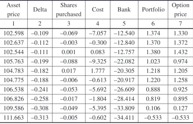
With the aim of hedging the short position, we consider a strategy that creates a long position in the option synthetically by buying or selling a certain quantity of shares given by the difference between the actual and the previous delta values (which stems from the theoretical calculations). Table 1 illustrates one realization of this delta hedging scheme considering a contract of one option. The hedging scheme performs three times per day, with the option being knocked out on the first rebalance (adjustment) of the fourth day. The asset price evolves as in column 1. Column 3 stems from column 2 and shows the buying or selling strategy. The cost of shares purchased (no transactions costs were assumed), as in column 4, creates a debt/credit in a bank account (col. 5). The theoretical option prices (col. 7) and delta values (col. 2) are computed via (2.19) and (2.20) respectively. We may note that the value of the delta-derived replicating portfolio (col. 6) tracks very well the option prices (col. 7).
Table 1: One realization of the delta hedging strategy (the barrier is breached on the first rebalance of the fourth day).
Asset
Delta Shares Cost Bank Portfolio Option
price purchased price
1 2 3 4 5 6 7
102.598 –0.109 –0.069 –7.057 –12.540 1.374 1.330
102.637 –0.112 –0.003 –0.300 –12.840 1.370 1.372
102.544 –0.111 0.001 0.083 –12.757 1.380 1.432
105.763 –0.199 –0.088 –9.325 –22.082 1.023 0.974
104.783 –0.182 0.017 1.777 –20.305 1.218 1.205
104.775 –0.188 –0.006 –0.613 –20.917 1.220 1.258
106.538 –0.241 –0.053 –5.692 –26.609 0.888 0.925
106.826 –0.258 –0.017 –1.804 –28.414 0.819 0.895
109.586 –0.308 –0.049 –5.395 –33.809 0.106 0.127
A novel definition of relative standard deviation of the hedging cost, which we denote σrel,
is established. It measures correctly the exposure of the practitioner to risk (enforced by the strategy), or else, the efficiency of risk absorbtion assigned to the strategy. The measure serves aiding the practitioner to adjust the number of rebalances during the option’s lifetime. Curiously, the notion that is present in the literature is different and looses the correct physical interpretation. Hence, we set
σrel =
σdelt a
σno
, (3.2)
whereσdelt a = E[(PT¯ −HT¯)2],σno = E[H0−HT¯)2], PT¯ is the value of the delta hedging
portfolio (which depends on the number of rebalances per day) and T¯ is either the expiration or the knock out time. Whence, σdelt a assigns the standard deviation of the hedge cost of the
delta hedging strategy andσno that of a strategy which is the nearest thing from doing nothing.
Indeed, the “no” strategy is characterized by the fact that the short seller hedges his position with the portfolio valued atH0totally invested in the money market account and do nothing more. In
this case, a hedgeper sedoes not exist in fact, as the dealer assumes 100% of the risk to settle his liability. So,σrel expresses the proportion of risk that must be assumed by the practitioner to
that absorbed by the delta hedging strategy (the text ahead illustrates the matter). The expression σdelta
H0 – usually found in the literature – does not provide such physical argument.
Remark. The mean value ofPT¯ −HT¯andH0−HT¯ are sufficiently small – as they should be
– so they are disregarded in (3.2).
Table 2 gives the relative standard deviations, the kurtosis and the asymmetry of hedge costs parameterized by the number of daily rebalances.
Table 2: Numerical results.
Rebalances
σrel σdelt a σno
Hedging
Curtosis Asymmetry
per day cost
1 0.43 1.125 0.382 0.0103 5.134 0.067
3 0.27 0.660 0.409 0.0022 7.903 0.017
6 0.20 0.474 0.422 0.0012 10.924 0.009
9 0.17 0.388 0.438 0.0013 14.361 0.103
12 0.15 0.338 0.444 0.0006 16.455 0.097
In periods of stability, the volatility will be small, so the values ofσrelwill decrease accordingly,
in which case, one rebalance per day or less would suffice. We note that the hedging cost, which assigns the gains/losses average in the long run, is almost zero, as it should be. We also notice that the kurtosis is greater than 3 and the asymmetry is small, for all rebalancing schemes.
4 CONCLUSION
Via the risk neutral pricing technique (no PDEs were involved), we have obtained closed-form expressions for the exact prices and hedges of an up-and-out call option with a constant barrier. We have assumed an arbitrary square integrable deterministic function of time to model the volatility and a zero interest rate for the riskless asset. This model is consistent with the fact that, in practice, traders often work with some devised deterministic behaviors for the volatility, as a guidance for their decision-making. It is noteworthy that the standard (constant) barrier option associated with this modeldoes notallow closed-form expressions.
The formulas provided recover verbatim standard results as particular cases, indicating that these are ready-to-use formulas leading to a minimum computational effort. Also, the results of the simulations were very good. The delta-derived replicating portfolio tracked very well the option prices. Underpinned by the novel definition of relative standard deviation, we established cor-rectly the proportion of risk assumed by the practitioner to that absorbed by the delta hedging strategy, as a function of the number of rebalances per day.
RESUMO.As quatro ´ultimas d´ecadas registraram um consider´avel esforc¸o de pesquisa na obtenc¸˜ao de formas fechadas para os prec¸os livres de arbitragem de vers ˜oes modificadas de opc¸˜oes europ´eias assim como para as estrat´egias associadas, permitindo-se tamb´em que a dinˆamica do ativo de risco subjacente exibisse parˆametros n˜ao necessariamente constantes. Nesse trabalho obtemos a forma fechada do prec¸o e da estrat´egia associada considerando uma opc¸˜ao com barreira up-and-outcom volatilidade representada por func¸˜oes determin´ısticas arbitr´arias. Particularizando-se a volatilidade para o caso constante, as express ˜oes resgatam as f´ormulas de Black & Scholes. Este fato sugere que o tempo de processamento computacional seja m´ınimo. Introduzimos tamb´em um novo crit´erio de desvio padr˜ao relativo para aferic¸˜ao da exposic¸˜ao do agente financeiro ao risco (induzido pela estrat´egia), posto que o crit´erio usual encontrado na literatura n˜ao traz uma correta interpretac¸˜ao f´ısica. A nova medida vem orientar o agente financeiro no ajuste do n´umero de intervenc¸˜oes no porfolio at´e a expirac¸˜ao da opc¸˜ao.
Palavras-chave: opc¸˜ao com barreira, prec¸os livres de arbitragem, medida Martingale, mudanc¸a de escala.
REFERENCES
[1] F. Black & M. Scholes. The pricing of options and corporate liabilities.J. of Political Economy,
[2] J. Cox & S. Ross. The valuation of options for alternative stochastic processes.Journal of Financial Economics,3(1976), 145–166.
[3] E. Derman & I. Kani. The ins and outs of barrier options: Part 1.Derivatives Quarterly, (1996), 55–67.
[4] J.M. Harisson & S.R. Plyska. Martingales and stochastic integrals in the theory of continuous trading. Stoch. Processes and their Applicatons,11(1981), 215–280.
[5] S.L. Heston. A closed-form solution for options with stochastic volatility with applications to bond and currency options.The review of Financial Studies,6(1993), 327–343.
[6] R. Heynen & H. Kat. Crossing the barrier.Risk,7(1994), 46–51.
[7] R. Heynen & H. Kat. Partial barrier options.Journal of Financial Eneneering3(1994), 253–274. [8] I. Karatzas & S.E. Shreve.Brownian Motion and Stochastic Calculus. Second Edition, Springer
(1991).
[9] A.W. Kolkiewicz. Pricing and hedging more general barrier options.J. of Computational Finance,
5(2002), 1–26.
[10] N. Kunitomo & M. Ikeda. Pricing options with curved boundaries.Mathematical Finance,2(1992), 275–298.
[11] Y. Kwok, L. Wu & H. Yu. Pricing multi-asset options with an external barrier.International Journal of Theoretical and Applied Finance,1(1998), 523–541.
[12] Y. Kwok.Mathematical Models of Financial Derivatives. Second Edition, Springer (2008).
[13] C.F. Lo, H.C. Lee & C.H. Hui. A simple approach for pricing barrier options with time-dependent parameters.Quant. Finance,3(2003), 98–107.
[14] C.F. Lo, H.M. Tang, K.C. Ku & C.H. Hui. Valuing time-dependent CEV barrier options.J. of Applied Mathematics and Decision Sciences, (2009), 1–17.
[15] C.F. Lo, P.H. Yuen & C.H. Hui. Constant elasticity of variance option pricing model with time-dependent parameters.International Journal of Theoretical and Applied Finance,3(2000), 661–674. [16] L.S.J. Luo. Various types of double-barrier options.J. of Computational Finance,4(2001), 125–138. [17] R.C. Merton. The theory of rational option pricing.Bell J. of Economics and Management Sciences,
4(1973), 141–183.
[18] D.R. Rich. The Mathematical Foundations of Barrier Option-Pricing Theory.Advances in Futures and Options Research,7(1994), 267–311.
[19] G. Roberts & C. Shortland. Pricing barrier options with time-dependent coefficients.Mathematical Finance,7(1997), 83–93.