Kondo Spin Splitting with Slave Boson
J. M. Aguiar Hualde,
Departamento de F´ısica J.J. Giambiagi, Facultad de Ciencias Exactas, Universidad de Buenos Aires, Ciudad Universitaria, 1428 Buenos Aires, Argentina.
G. Chiappe,
Departamento de F´ısica Aplicada, Unidad Asociada del Consejo Superior de Investigaciones Cient´ıficas and Instituto Universitario de Materiales, Universidad de Alicante, San Vicente del Raspeig, Alicante 03690, Spain. and
Departamento de F´ısica J.J. Giambiagi, Facultad de Ciencias Exactas, Universidad de Buenos Aires, Ciudad Universitaria, 1428 Buenos Aires, Argentina.
E.V. Anda
Departamento de F´ısica, Pontificia Universidade Cat´olica do R´ıo de Janeiro, 22452-970 R´ıo de Janeiro, Caixa Postal 38071, Brasil.
Received on 8 December, 2005
The slave boson (SB) technique is employed to study the Zeeman spin splitting in a quantum dot. Unlike traditional SB method, each spin is renormalized differently. Two geometries are compared: side connected and embedded. In both cases, it’s shown a non linear behavior of the splitting as a function of the magnetic field applied. The results are in line with the latest experiments.
Keywords: Kondo effect; Nanoscopic systems
I. INTRODUCTION
When a spin is localized in a quantum dot (QD) coupled to metallic leads, local spin fluctuations (LSF) produce the spin of electrons in the leads to screen the localized spin giving rise to the Kondo Effect (KE) in a similar way as it happens on a magnetic impurity in a host metal. The KE was first theoretically proposed in [3] and was observed in quantum dots in [1, 2]. When this effect takes place, a sharp resonance in the local density of states is developed at the Fermi level of the system.
If a magnetic field is applied on the QD, the LSF are quenched and the Kondo Regime (KR) tends to disappear which produces the resonance to split in first place and to van-ish later for a strong enough magnetic field. All these effects have consequences observable in the differential conductance of the system.
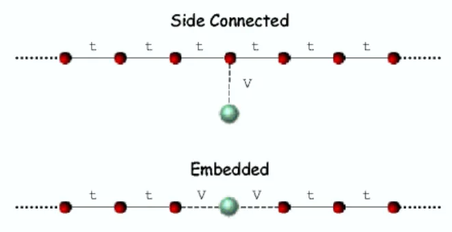
The way in which the QD is coupled to the leads plays an important role in the action of the KE on the system. It’s been considered two geometries depicted in Fig. 1. In an embed-ded geometry (EG), in which the QD is between two leads, the resonance provides a channel of conduction and the con-ductance reaches the value G=2e2/h=2G0. On the other hand, in a side connected geometry (SCG), the QD is coupled to one site of an infinite linear chain and the resonance pro-duces a channel of conduction that interferes with the direct channel of the chain causing the conductance to vanish for a particular value of the gate potential.
In recent experiments it was possible to do a precise mea-sure of∆, the Zeeman spin splitting (ZS), for a QD in the KR [5, 6]. The main results of these experiments seems to be con-troversial: while in the former [2] is found∆∼∆B=2gµBB (where 2∆Bis the magnetic Zeeman energy,gis the
gyromag-FIG. 1: Sketch of the geometry of the two topologies considered in this work. Upper panel, SCG. Lower panel, EG.
netic factor,µB is the Bohr magneton, andBis the magnetic field) and begins after a critical field is reached (Bc), in the last the existence of a critical field is also observed, but the split-ting is larger than∆Band does not extrapolate to zero at zero field. As a consequence,∆BatBcresults significantly lower thankBTK, beingTKthe Kondo temperature.
screening characteristic of the KR should reduce the magnetic field splitting,i.e∆<∆B. Unfortunately these theories were not capable of explaining the phenomenology seen in the lat-est experiments.
In order to obtain the experimental behavior of∆, it was employed the SB method in a new way. Unlike traditional SB [10] and similar X-boson approach [4], each spin species was renormalized differently. This allows to show in a natural way how magnetization merges in the system when a mag-netic field is applied.
In the following section the new slave boson method is ex-plained and it’s shown the relevant quantities considered in this proceeding. Next, the results obtained are presented and it’s given a discussion from them. Finally, the relevant points are summarized.
II. METHOD
The system is modeled with the Anderson impurity Hamil-tonian with magnetic field and infinite Coulomb repulsion at the QD which is labeled as site 0 in both of the geometries. It can be identified three parts: the leads (
H
L), the QD (H
QD) and the connection between them (H
T). The leads parts cor-respond to an infinite linear chain in SCG and to two semi infinite ones in the EG case. The other two parts readsH
QD =∑
σ
εσnˆ0σ+Unˆ0↑nˆ0↓;εσ=
½
Vg+B σ=↑
Vg−B σ=↓
H
T =∑
iσ
V(a†iσa0σ+a†0σaiσ),
σ = {↑,↓}; ˆn0σ=a†0σa0σ;i=
½
−1,1 EG
1 SCG
whereVgis the gate potential at the QD site,Uis the Coulomb repulsion taken infinite for calculations andV is the hopping between the QD and the leads. It’s adopted|gµB|=1 and all energies are expressed in units of the hopping of linear chain (t=1, see Fig. 1), therefore the bandwidth isD=4.
The new SB method consists in defining a boson field as-sociate to each electron spin which introduces states that can only be occupied by a spinσ but not by ¯σ. This way, the fermion operators are replaced by a product of a new fermion (c) and a boson (b) operators
a†0σ7→c†0σb†σ. (1) In order to avoid double occupancy in the QD, it must be imposed two constrain conditions
2 ˆn0σ+bσ†¯bσ¯−b†σbσ+b†σbσbσ†¯bσ¯=1. (2) Note that when both of the spins species are equivalent, the above equations merges in the usual constrain of the SB for-malism [10] where the probability that the site is empty is the product of the probabilities of being empty of spin up and spin down. Next, mean value is taken in (2) and the boson operators are treated in mean field approximation; defining
zσ=hbσi and taking the Fermi energy εF =0 to compute
hnˆ0σi=n0σ, the above equation results
2n0σ+z2σ¯−z2σ+z2σz2σ¯=1. (3) Incorporating (3) to the Hamiltonian through Lagrange multipliersγ↑andγ↓, two more conditions are obtained (one for each spin specie) minimizing it respect tozσ:
KVha†1σc0σi+z2σ¯(γσ+γσ¯) +γσ¯−γσ=0;K=
½
1 SCG 2 EG
(4) This way, a non linear system of 4 equations is posed. This system is numerically solved and the parametersγσandzσare obtained. These values determine the Hamiltonian and then diagonal and non diagonal elements of the Green function are calculated. Particularly, it’s specialized the Green function at the QD
G0σ(
E
) =1/[E
−εσ−2γσ−K(V zσ)2gL(E
)], (5) which presents a resonance at the Fermi level due to the renor-malization of the energy. This resonance has a width given byW=K
· (V z
↓)2
1−(K−1)(V z↓)2+
(V z↑)2 1−(K−1)(V z↑)2
¸ (6)
what will be useful to discriminate the Kondo Regime. In the expression ofG0σ(
E
)(5), gL(E
) is the undressed Green function of the leads which in each geometry is explic-itly:gL(
E
) =
EG: SCG:
E+√E2−4t2 2t2
1 √
E2−4t2 :
E
<−2tE−i√4t2−E2 2t2 √ −i
4t2−E2 :−2t<
E
<2tE−√E2−4t2 2t2 √−1
E2−4t2 : 2t<
E
. (7)
Observe that, inside the band,gL(
E
)has real and imaginary part for the EG but is purely imaginary for the SCG case. Due to this, the renormalized energies of the QD levelEσ= εσ+2γσ
1−(K−1)(V zσ)2, (8) has a factor correction only for the EG. The quantity
Γσ=
2γσ
1−(K−1)(V zσ)2, (9) can be interpreted as the renormalization of the energy level by the interaction. This interaction dependent renormalization is different for up and down levels what gives an additional contribution to the splitting
∆=E↓−E↑= Vg+B+2γ↓
1−(K−1)(V z↓)2−
Vg+B+2γ↑ 1−(K−1)(V z↑)2.
(10) From this last expression, it can be noted that in the SCG (K= 1),Vgdoesn’t affect the splitting∆.
-0.1 0 0.1 0.2 0.3
0 0.005 0.01 0.015 0.02 0.025
∆
/2
B
Opposed;Vg=-0.5 Aligned;Vg=-0.5 No Mag.;Vg=-0.5 Average;Vg=-0.5 Vg=-0.3
0 0.1 0.2 0.3 0.4 0.5 0.6 0.7 0.8 0.9
0 0.005 0.01 0.015 0.02 0.025
Parameters
B
z↓ z↑ ∆n ∆Γ
0 0.02 0.04 0.06 0.08 0.1 0.12 0.14
0 0.005 0.01 0.015 0.02 0.025
∆
/2 and Width
B
Resonance width Averaged Solution
0 0.2 0.4 0.6 0.8 1 1.2 1.4 1.6 1.8 2
-1 -0.5 0 0.5 1
Transmission
E
B = 0.00 B = 0.01 B = 0.02
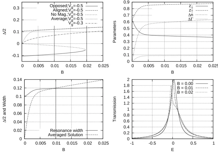
FIG. 2: Embedded geometry. From left to right and top to bottom: Three solutions found for∆and the average as a function ofB, parameter evolution withBand values for∆Γmagnetization∆n, resonance width and splitting compared, transmission as a function ofE for three
magnetic field values.Vg=−0.5 in all panels except the first. The fields at which transmission is plotted are indicated with vertical lines.
III. RESULTS
The values ofV were chosen in both geometries in such a way they gave approximately the same Kondo resonance (0.35 in the EG and 0.65 in the SCG).
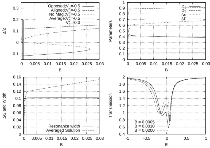
In the first panel of Figs. 2 and 3 is plotted the splitting∆as a function ofB. When the gate potential is not much low, the solution is unique corresponding to the magnetization aligned with the magnetic field applied but, when the gate potential was low enough, it was found a magnetic field value below which there were three solution regimes. One of them cor-responds to a solution in which the magnetization is aligned with the magnetic field and has the lowest energy; the solution with the magnetization opposed to the field has the highest en-ergy and the last one, which corresponds to a solution with low magnetization, has an intermediate value of energy. This or-der changes at zero field; the lowest energy is for the solution with low magnetization while the other two have the same en-ergy. It can be seen that in both of the geometries there are three solutions withVg=−0.5 and only one withVg=−0.3.
The final solution was obtained averaging each quantity weighted with a Boltzmann factor introducing a little temper-aturekBT =10−6much less than the width of the resonance
(6)
hAi = ∑ 3
i=1CiAi
∑3i=1Ci
; Ci=e−(Ei−Emin)/kT, (11)
Ai = {zσi,εσi,nσi,∆Γi,∆ni}. (12) Here,ilabels each one of the three found solutions.
The results in Figs. (2) and (3) show that∆ grows much more fast at low fields than expected whenVgis lowered. This is due to the different renormalization produced by the inter-action in each spin energy level.
The resonance width (6) resulted to lie between approxi-mately(0.1−0.12)in EG and between(0.09−0.1)in SCG, which is in line with the Kondo temperature obtained with the formula [11]
kBTK=D exp
µ −x|Vg|
2KV2 ¶
; x= ½
2π SCG
π EG (13)
since it is approximatelykBTK ≈0.08. Therefore, it can be said that the resonance width is practically the Kondo temper-ature.
-0.1 0 0.1 0.2 0.3
0 0.005 0.01 0.015 0.02 0.025 0.03
∆
/2
B
Opposed;Vg=-0.5 Aligned;Vg=-0.5 No Mag.;Vg=-0.5 Average;Vg=-0.5 Vg=-0.3
0 0.1 0.2 0.3 0.4 0.5 0.6 0.7 0.8 0.9 1
0 0.005 0.01 0.015 0.02 0.025 0.03
Parameters
B
z↓ z↑ ∆n ∆Γ
0 0.02 0.04 0.06 0.08 0.1 0.12 0.14 0.16
0 0.005 0.01 0.015 0.02 0.025 0.03
∆
/2 and Width
B
Resonance width Averaged Solution
0.4 0.6 0.8 1 1.2 1.4 1.6 1.8 2
-1 -0.5 0 0.5 1
Transmission
E B = 0.0005 B = 0.0010 B = 0.0200
FIG. 3: Side connected geometry. From left to right and top to bottom: Three solutions found for∆and the average as a function ofB, parameter evolution withBand values for∆Γmagnetization∆n, resonance width and splitting compared, transmission as a function ofE for
three magnetic field values.Vg=−0.5 in all panels except the first. The fields at which transmission is plotted are indicated with vertical lines.
then continue evolving asymptoticallyz↑→1 andz↓→0. The magnetization
∆n=n0↑−n0↓ (14)
and the difference
∆Γ=Γ↑−Γ↓= 2γ↑
1−(K−1)(V z↑)2−
2γ↓ 1−(K−1)(V z↓)2
(15) also show the same initial fast growth and then a slow varia-tion.
The conductance is as it was expected: in the EG reaches the value 2G0=2e2/hat
E
=0 forB=0 what indicates that the quantum dot favors the conduction while, in the SCG, it tends to vanish atE
=0 as the field decrease.In order to quantify the moment at which the splitting can be appreciated, it was plotted together the averaged solution and the resonance width. In the EG, the field value at which the splitting is well resoluted results to be approximately the same field at which the solution with spin opposed to the field disappears. On the other hand, in SCG, the splitting is well defined practically from beginning. This behavior is under-stood analyzing the splitting (10): in the EG (K=2) there’s a
negative contribution to∆that comes fromVgbut, in the SCG (K=1) there’s no contribution fromVg and the splitting is appreciable long before that in the EG case.
IV. SUMMARY
We have developed a new slave boson formalism that takes into account the spin polarization in a magnetic field. The Kondo resonance with this new method is wider respect to the traditional SB method since the boson’s occupation in this last one is the product of the occupation for the boson up and boson down in our SB scheme.
Under the action of a magnetic field, the energy levels up and down undergo a different renormalization by effect of the interactions. This gives an additional contribution to the
split-ting∆, with the interactions as its origin, and whose precise
value depends on the topology of the circuit.
intercepts the origin. As a result of this, the critical field at which the splitting of Kondo resonance begins to be seen, is lower than that expected from comparing the Zeeman energy with the scale of energy associated to the Kondo Temperature kBTK. This critical field also resulted strongly dependent of the circuit topology. For the EG, there’s an additional con-tribution proportional to the gate potential which makes the levels separation to be slower than in the SCG, making grow this way the critical field.
All this is in line with the results of the last experiments [5, 6].
Acknowledgments
Financial support by the Argentinian CONICET and UBA (grant UBACYT x115) and the spanish program Ramon y Cajal of MCyT are gratefully acknowledged. Also fund-ing from Generalitat Valenciana, GV05/152 and to grant FIS200402356 of MCYT are gratefully acknowledged.
[1] D. Goldhaber-Gordon, H. S. Shtrikman, D. Mahalu, D. Abusch-Magder, U. Meirav, and M. A. KASTNER, Nature 391, 156 (1998).
[2] S.M. Cronenwett, T. H. Oosterkamp, and L. P. Kouwenhoven, Science281, 540 (1998).
[3] T.K. Ng and P. A. Lee, Phys. Rev. Lett.61, 1768 (1988). [4] R. Franco R, M. S. Figueira, and E. V. Anda, Phys. Rev. B67,
155301 (2003)
[5] A. Kogan, S. Amasha, D. Goldhaber-Gordon, G. Granger, M. A. Kastner, and H. Shtrikman, Phys. Rev. Lett. 93, 166602 (2004).
[6] S. Amashaet.al, cond. mat. 0411485 (2005).
[7] Y. Meir, N.S. Wingreen, and P.A. Lee Phys. Rev. Lett.70, 2601 (1993).
[8] T.A. Costi, Phys. Rev. Lett.85, 1504 (2000).
[9] J.E. Moore and X.-G. Wen, Phys. Rev. Lett.85, 1722 (2000) [10] P. Fulde, in Electron Correlations in Molecules and Solids
Springer; 3 edition (April 25, 2003)