Computer Simulation of Dynamical Anomalies in Stretched Water
P. A. Netz
a, F. Starr
b, M. C. Barbosa
c, and H. Eugene Stanley
d aDepartamento de Qu´ımica, ULBRA, Canoas RS, Brasil and Departamento de Qu´ımica, Unilasalle, Canoas RS, Brasil; b
Center for Theoretical and Computational Materials Science and Polymers Division,
National Institute of Standards and Technology, Gaithersburg, Maryland 20899, USA; c
Departamento de F´ısica, UFRGS, Porto Alegre RS, Brasil; d
Center of Polymer Studies - Boston University Boston, MA 02215, USA
Received on 02 September, 2003.
In this work, we describe how the anomalous diffusivity is related to the structural anomalies. For this purpose, we study how the thermodynamics and the dynamics of low-temperature water are affected by the decrease of the density.
1
Introduction
Water is one of the most important substances in nature, and its remarkably complex behavior is puzzling, specially when we consider the simplicity of the chemical structure of wa-ter’s molecule [1-4]. Water behaves anomously in several ways[5]: it expands on freezing and therefore has a negative slope in the solid-liquid equilibrium line in the P-T diagram. Under atmospheric pressure, water has a density maximum at 4oC, a minimum in the isothermal compressibility at 46 o
C, and a minimum in the isobaric heat capacity at 35oC. It has usually high melting, boiling and critical points, among several other anomalies[6, 7].
It is known that these anomalies, as well as the main properties of water, including the properties that make water the essential fluid in biological systems, are linked to the mi-croscopic structure of water and the peculiar intermolecular interactions. Nonetheless, it remains astonishing, how does this complex behavior emerge from a simple structure. The reproduction of the anomalous behavior and the description of these complexities is a challenge not only to the computer simulations, but also to the theoreticians that are developing theories for the mechanisms that govern complex systems. And in this aspect, computer simulations have been sucess-full in reproducing a wide range of properties of water and several anomalies, starting with very simple models.
Particularly, it is already known that there are three kinds of anomalies[8]: thermodynamic, dynamical and structural. The region in the phase diagram where the first kind of anomaly occurs is entirely inside the domain of the second, which in its turn within the region of the third. Inside the region of structural anomalies, the orientational and transla-tional order show inter-dependence[8]. A key point is, there-fore, to discover how does the structure affect the mobility.
The complex behavior of water can be approached both from the thermodynamic as well as from the microscopic
level. Let us begin by focusing in the thermodynamical as-pects. There are three possible explanations for the anoma-lous increase of the thermodynamic response functions (such as isothermal compressibility, isobaric heat capacity) on cooling, namely, the stability limit conjecture [9-11], the critical point hypothesis [12-15] and the singularity-free hy-pothesis [16-18]. According to the stability-limit conjec-ture, the increase in the thermodynamic response functions on cooling can be explained supposing that the curves are close to the spinodal, the line separating the region in the phase diagram where the liquid phase is metastable from the region where it is unstable. The pressure in the liquid spinodal in water’s phase diagram, according to this con-jecture, decreases on cooling, but attains a minimum value (at negative pressures). The spinodal reenters the positive pressures region of the phase diagram with further cooling, being in this way called a reentrant spinodal. The critical point hypothesis explains the anomalous increase in the re-sponse functions as being due to the proximity of a second critical point, which is located probably at - 85oC and 230
be-havior can be obtained by studying supercooled water under negative pressures (stretching). Fluids under negative pres-sures are relevant not only from the academic point-of-view (it is not merely an academic curiosity), but also play an important role on realistic system, such as in the transport of water in plants[23]. Experimental results [24-26] as well as computer simulations [27-35] show that, starting with at-mospheric conditions of pressure, the gradual increase of pressure increases the number of defects such as multiple H-bonds and interstitial water molecules, disrupting the tetra-hedral local structure and leading to a weakening of the H-bonds and therefore to an increase in the mobility [32-39]. Applying very high pressures, however, leads to steric ef-fects which lower the mobility, and as a result the diffusion constant attains a maximum at a given densityρmax. Above
ρmax, the diffusion of water is controlled by hindrance, with
the hydrogen bonds playing a secondary role. We show that a complementary behavior is found if water is submitted to a gradual decrease in pressure, from atmospheric to negative pressures, with a minimum of diffusivity at a given density
ρmin, as discussed in details further in this paper.
There are many different models used in the computer simulation, and the differences between them were recently reviewed[40, 41] None of them can reproduce exactly all of water properties and anomalies. Even though, the over-all thermodynamic picture that emerges from different com-puter simulation models is roughly the same, but the dy-namic properties are slightly more model-dependent. From the large diversity of potentials, the potentials with three in-teraction centers are computationally faster. Among them the SPC/E[42] is particularly accurate in the description of thermodynamic and dynamical properties of water and is largely used in pure water simulations as well as in biolog-ical systems. It is also known that the SPC/E water model can reproduce the maximum in diffusivity under pressure as well as the power-law behavior of dynamical properties on cooling and therefore it seems to be a good choice for ana-lyzing the dynamics of stretched water.
In this work, we will describe how the anomalous dif-fusivity is related to the structural anomalies. For this pur-pose, we study how the thermodynamics and the dynamics of low-temperature water are affected by the decrease of the density.
2
Methods
We performed an extensive set of molecular dynamics simu-lations using 216 SPC/E [42] water molecules. The Newton equations of motion were integrated using SHAKE [43, 44] with time steps of 1.0 fs for T>210 K and 2.0 fs for T = 210 K. The range of temperatures and densities covered was 210 K< T <280 K and 0.825 g/cm3
< ρ <1.30 g/cm3
. Many state points in this range have negative pressure, and at low densities they are either a metastable stretched liq-uid, or a phase separated liquid-gas mixture. All simula-tions were carried out in the canonical ensemble (NVT), in
a cubic simulation box using periodic boundary conditions. The rescaling of the velocities was made using the Berend-sen thermostat [45], the electrostatic interactions were cal-culated using reaction field [46] with cut-off radius of0.79
nm.
The diffusion coefficient D was calculated from the asymptotic slope of the mean square displacement plotted versus time:
D= 1 6
dhr2
(t)i
dt (1)
The orientational relaxation was analyzed using the ro-tational autocorrelation functions [43]:
C(e) =he(t)·e(0)i (2)
The vectoreis a chosen unity vector describing the ori-entation of the dipole moment. Other possible choices of unity vectors such as the O-H bond direction and the vec-tor perpendicular to the plane of the molecule give similar results[48]. The orientational relaxation time was calculated from these functions using an biexponential decay fit func-tion. [47]
C=a0exp(−bt 2
/2) +aIexp(−t/τI) +aIIexp(−t/τII)
(3) The first term correspond to a fast librational motion, and the two relaxation times take into account the possibil-ity of a fast and a slow reorientation process. However, in the most of the cases taking only one exponential yielded a reasonable result, and thus only one relaxation time was determined.
In order to understand the effect of the structure on the dynamics we also carried out a detailed analysis of the lo-cal structure of water [49] computing the distribution of the number and angle of H-bonds (O-H· · · O) and distribution of the number and angle of first neighbor molecules, analyz-ing the angle O· · · O· · · O. The number of first neighbors is calculated by computing all molecules whose distance from a given molecule is less than 0.32 nm. This distance repre-sents the first minimum in the oxygen-oxygen radial distri-bution functiongOO(r)at moderate and low densities. In
order to have a better comparison, the same O-O distance criterion is also applied for all state points, irrespective the density.
3
Results
3.1
Thermodynamic Properties
Table 1 shows the thermodynamic properties obtained in our MD simulations. A crucial point in the distinction between
Table 1. Thermodynamic properties: temperature, density, poten-tial energy and pressure. The errorbars in the energy are about 0.2 and in the pressure, about 15-20
T (K) ρ(g/cm3) U (kJ/mol) P (MPa) 280 0.850 - 47.01 - 239
0.875 - 47.32 - 230 0.900 - 47.75 - 204 0.925 - 47.90 - 172 1.125 - 48.86 320 260 0.850 - 48.53 - 261
0.875 - 48.88 - 257 0.900 - 49.23 - 231 0.925 - 49.48 - 191 1.125 - 50.01 289 250 0.850 - 49.28 - 273
0.875 - 49.76 - 271 0.900 - 50.03 - 244 0.950 - 50.40 - 148 240 0.850 - 50.17 - 263 0.875 - 50.51 - 282 0.900 - 50.98 - 258 0.925 - 51.30 - 213 0.950 - 51.26 - 155 0.975 - 51.32 - 102 1.000 - 51.38 - 36 1.075 - 51.31 134 1.125 - 51.27 271 1.250 - 51.24 758 1.300 - 51.26 1042 230 0.850 - 51.06 - 278 0.875 - 51.28 - 300 0.900 - 51.80 - 272 0.925 - 52.01 - 212 1.125 - 51.92 230 220 0.900 - 52.62 - 278
0.925 - 53.14 - 221 210 0.850 - 53.15 - 344 0.875 - 52.92 - 348 0.925 - 53.55 - 225
the different thermodynamic scenarios, the stability-limit conjecture the critical point and the singularity-free hy-potheses, is the shape of the spinodal. Computer sim-ulations help us to locate the spinodal. We fit the P
-ρ isotherms with a fifth-order polynomial and locate the minima in each isotherm, where the isothermal compress-ibility is zero. These minima define the stability limit beyond which no equilibrium exists and therefore it lo-cates the spinodal Psp(T). We found a non-reentrant
spinodal[53], qualitatively similar to that found by Harring-ton and coworkers[31]. The same result was also found by
Yamada and coworkers [54-56] using the TIP5P[57] poten-tial. This behavior can support both the critical point hy-pothesis and the singularity-free scenario.
The density at the spinodalρsp(T) was calculated as well
and is located in a narrow range 0.853≤ρsp≤0.874. For
our results that means that our simulated points whose den-sity is less than 0.875 either should be ruled out or care must be taken in order to check the evidence of cavitation.
3.2
Dynamic Properties
The translational diffusion coefficient (D) and the orienta-tional relaxation time (τ) of SPC/E water were analyzed. Table 2 shows the dynamic properties of the simulated state points. Fig. 1 showsD along isotherms. ForT ≤260 K,
Dhas a minimum at aboutρ≈0.9 (g/cm3
), which becomes more pronounced at lower temperatures. The rotational dif-fusion (orientational relaxation time) displays a very similar trend, as shown in Fig. 2. The behavior ofτalong isotherms is in fact complementar to the behavior ofD. The relaxation time τ initially increases, with decreasing density, passes through a maximum and decreases with further stretching. the maximum in τ can be found in the same region as the minimum inD. The productτ×D(not shown) is remark-ably constant irrespective the temperature or density[58, 50].
0.8 0.9 1 1.1
ρ (g / cm3 )
0 0.2 0.4 0.6
D (10
-5cm 2 /s )
Figure 1. Diffusion Coefficient versus Density for temperatures
T = 230K (circles), T = 240K (squares),T = 250K
(dia-monds) andT = 260K(triangles).
0.8 0.9 1 1.1
ρ (g / cm3 ) 0
100 200 300
τ
(ps )
Figure 2. Orientational Relaxation Time versus Density for tem-peraturesT = 230K(circles),T = 240K(squares),T = 250K
Table 2. Temperature, density, diffusion coefficient and orienta-tional relaxation time for the dipole vector.
T (K) ρ(g/cm3
) D(10−5cm2/s) τ(ps)
280 0.850 1.359 9.16 0.875 1.281 9.19 0.900 1.261 9.46 0.925 1.234 9.12 1.125 1.158 6.59 260 0.850 0.634 23.91
0.875 0.531 23.47 0.900 0.527 22.16 0.925 0.500 26.93 1.125 0.635 12.35 250 0.850 0.346 40.00 0.875 0.298 47.69 0.900 0.295 43.89 0.950 0.281 38.73 240 0.875 0.130 95.89 0.900 0.105 118.7 0.925 0.122 103.8 0.950 0.149 75.37 0.975 0.178 66.06 1.000 0.210 56.63 1.075 0.293 34.71 1.125 0.291 28.85 1.250 0.210 27.73 1.300 0.153 35.29 230 0.850 0.0674 216.8 0.875 0.0601 239.8 0.900 0.0435 314.3 0.925 0.048 238.8 1.125 0.178 48.61 220 0.900 0.0114 623.9 0.925 0.00612 1208 210 0.850 0.0019 9229 0.875 0.00373 3582 0.925 0.00303 3441
These results show that the stretching has influence both in the translational as well as in the rotational diffusion. The complementar behavior of translational and rotational dif-fusion should be interpreted not in terms of hydrodynamic arguments[59], but rather as a clue pointing out that both the translational diffusion as well as the orientational pro-cess involve microscopic rearrangements, i.e. both motions are correlated by a common mechanism. In order to better understand this mechanism, the detailed microscopic struc-ture of water was also investigated.
3.3
Structural Properties
One important aspect about molecular dynamics simulations is the very detailed microscopic information that these sim-ulations can give. For instance, it is possible to look at the neighbor structure of each water molecule at each simula-tion step, obtaining a statistical picture of the local structure. Several aspects can be investigated, such as the distribution of the number of neighbors and number of H-bonds and also
the angle distribution of neighbor molecules (O· · · O· · · O) angle and angle distribution of H-bonds.
Table 3 shows the distribution of the number of neigh-bors and H-bonds for the simulated state points. Fig. 3 shows the H-bond and O· · · O · · · O angle distributions for the temperatureT= 240 K, at several densities, whereas the same properties, analysed fixing the density atρ= 0.90 g/cm3
and atρ= 1.125 g/cm3
at several temperatures were shown in Figs. 4 and 5, respectively.
0 30 60 90
angle (degrees) 0
0.01 0.02 0.03 0.04 0.05
H-bond distribution
0 30 60 90 120 150 180 angle (degrees)
0 0.005 0.01 0.015 0.02
O...O...O distribution
Figure 3. (a) Hydrogen bond angle distribution and (b) neighbors
O· · ·O· · ·Oangle distribution for several densities at the
tem-perature T = 240 K. Shown are the results forρ= 0.900 g cm−3
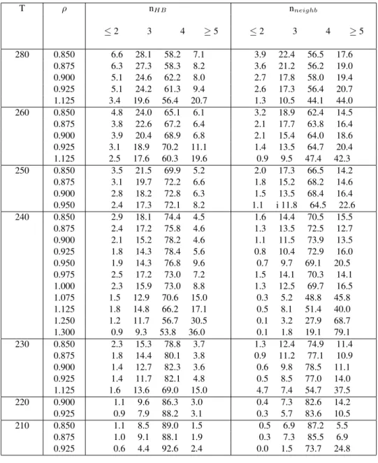
Table 3. Results of the simulations. Distribution of the number of H bonds and neighbors.
T ρ nHB nneighb
≤2 3 4 ≥5 ≤2 3 4 ≥5
280 0.850 6.6 28.1 58.2 7.1 3.9 22.4 56.5 17.6 0.875 6.3 27.3 58.3 8.2 3.6 21.2 56.2 19.0 0.900 5.1 24.6 62.2 8.0 2.7 17.8 58.0 19.4 0.925 5.1 24.2 61.3 9.4 2.6 17.3 56.4 20.7 1.125 3.4 19.6 56.4 20.7 1.3 10.5 44.1 44.0 260 0.850 4.8 24.0 65.1 6.1 3.2 18.9 62.4 14.5 0.875 3.8 22.6 67.2 6.4 2.1 17.7 63.8 16.4 0.900 3.9 20.4 68.9 6.8 2.1 15.4 64.0 18.6 0.925 3.1 18.9 70.2 11.1 1.4 13.5 64.7 20.4 1.125 2.5 17.6 60.3 19.6 0.9 9.5 47.4 42.3 250 0.850 3.5 21.5 69.9 5.2 2.0 17.3 66.5 14.2
0.875 3.1 19.7 72.2 6.6 1.8 15.2 68.2 14.6 0.900 2.8 18.2 72.8 6.3 1.5 13.5 68.4 16.4 0.950 2.4 17.3 72.1 8.2 1.1 i 11.8 64.5 22.6 240 0.850 2.9 18.1 74.4 4.5 1.6 14.4 70.5 15.5
0.875 2.4 17.2 75.8 4.6 1.3 13.5 72.5 12.7 0.900 2.1 15.2 78.2 4.6 1.1 11.5 73.9 13.5 0.925 1.8 14.3 78.4 5.6 0.8 10.4 72.9 16.0 0.950 1.9 14.3 76.8 9.6 0.7 9.7 69.1 20.5 0.975 2.5 17.2 73.0 7.2 1.5 14.1 70.3 14.1 1.000 2.3 15.9 73.0 8.8 1.3 12.5 69.7 16.5 1.075 1.5 12.9 70.6 15.0 0.3 5.2 48.8 45.8 1.125 1.8 14.8 66.2 17.1 0.5 8.1 51.4 40.0 1.250 1.2 11.7 56.7 30.5 0.1 3.2 27.9 68.7 1.300 0.9 9.3 53.8 36.0 0.1 1.8 19.1 79.1 230 0.850 2.3 15.3 78.8 3.7 1.3 12.4 74.9 11.4
0.875 1.8 14.4 80.1 3.8 0.9 11.2 77.1 10.9 0.900 1.4 12.7 82.3 3.6 0.6 9.8 78.5 11.1 0.925 1.4 11.7 82.1 4.8 0.5 8.5 77.0 14.0 1.125 1.6 13.6 69.0 15.0 4.7 7.4 54.7 37.5 220 0.900 1.1 9.6 86.3 3.0 0.4 7.3 82.6 14.2 0.925 0.9 7.9 88.2 3.1 0.3 5.7 83.6 10.5 210 0.850 1.1 8.5 89.0 1.5 0.5 6.9 87.2 5.5
0.875 1.0 9.1 88.1 1.9 0.3 7.3 85.5 6.9 0.925 0.6 4.4 92.6 2.4 0.0 1.5 73.7 24.8
0 30 60 90
angle (degrees) 0
0.01 0.02 0.03 0.04 0.05
H-bond distribution
0 30 60 90 120 150 180
angle (degrees) 0
0.005 0.01 0.015 0.02 0.025
O...O...O distribution
Figure 4. The same as Fig. 3, but for several temperatures at fixedρ= 0.900 g cm−3. Shown are the results for T = 230 K
0 30 60 90 angle (degrees)
0 0.01 0.02 0.03 0.04
H-bond distribution
0 30 60 90 120 150 180
angle (degrees) 0
0.005 0.01 0.015
O...O...O distribution
Figure 5. The same as Fig. 4, but forρ= 1.125 g cm−3. The symbols are the same as in Fig. 4.
The detailed analysis of the local structure of water re-veals the enhancement of the tetrahedrality at low tempera-tures and ice-like densities. This can be detected from the angle distributions shown in these figures. Lowering the density, the O· · · O· · · O angle distribution becomes more sharply peaked around the tetrahedral angle, indicating an enhancement of the ice-like structure. the peak around 60o, on the other side, is related to a fifth neighbor in the coordi-nation shell and the presence of this fifth neighbor increases with increasing density, as shown in Fig. 3b and Table 3. At very high densities, a peak appears around 80o, related to the appearance of a 6th neighbor[50]. The O · · · O· · · O angle distribution, at a fixed density, seems to depend only weakly on temperature, as shown in Figs. 4b and 5b.
The H-bond angle distribution, indicated in Fig. 3a seems not to depend on density, as far as this density is not too high. Fixing the density and analyzing the effect of tem-perature (as in Figs. 4a and 5a) we see that the peaks become broad with increasing T, indicating only a thermal fluctua-tion. Only at very high densities does the H bond become distorted.
The increase of the number of molecules with higher co-ordination numbers at densities ranging between ρmin and
ρmax is responsible for the increase on the diffusion
coef-ficient with increasing density. The number of H-bonds, however, does not alter significantly, meaning that these imperfections arise from the inclusion of extra molecules in the coordination shell which either do not for H-bonds or share and H-bond with another molecule. This shared bonds are weakened and the molecule can connect to an-other molecule by means of a small rotation, keeping the remaining H-bonds. The net motion of water structure can be described as a slow non-oscillatory or quasi-oscillatory translational and rotational displacements[60]. This
pecu-liar mechanism can explain the coupling between transla-tional and rotatransla-tional diffusion, without the need of invoking hydrodynamical arguments.
4
Conclusions
In conclusion, we propose that the anomalous dynamic be-havior of supercooled water can be explain in terms of its structural properties: the number and the distribution of hy-drogen bonds and and the number and angular distribution of the O-O-O neighbors. We calculate these quantities for a wide range of densities and temperatures. We observe that the number of molecules with four neighbors has a maxi-mum at the densityρmin where the translational diffusion
has a minimum and the rotational diffusion is maximum. Forρmax, the density of highest translational diffusion, the
prob-ability to find these extra molecules in the neighborhood of a given molecule, and therefore the translational and rota-tional diffusion are slow.
References
[1] D. Eisenberg and W.J. Kauzmann. The Structure and Prop-erties of Water. Clarendon, London, 1969.
[2] P. Ball. Life’s Matrix: A Biography of Water. Farrar Straus and Giroux, New York, 2000.
[3] V. Brazhkin, S.V. Buldyrev, V.N Ryzhov, and H.E. Stanley, editors.New Kinds of Phase Transitions: Transformations in disordered systems, Dordrecht, 2002. NATO Advanced Re-search Workshop, Volga River, Kluwer.
[4] O. Mishima and H.E. Stanley. Nature,392, 164 (1998).
[5] Martin Chaplin. Water structure and behavior, http://www.sbu.ac.uk/water.
[6] E.W. Lang and H.-D. L¨udemann.Angewandte Chemie, Inter-national Edition in English,21, 315 (1982).
[7] R.C. Dougherty and L.N. Howard. Journal of Chemical Physics,109, 7379 (1998).
[8] J. R. Errington and P. G. Debenedetti. Nature,409, 318 Jan-uary (2001).
[9] R.J. Speedy. Journal of Physical Chemistry,86, 982 (1982).
[10] R.J. Speedy. Journal of Physical Chemistry,86, 3002 (1982).
[11] R.J. Speedy. Journal of Physical Chemistry,91, 3354 (1987).
[12] P. H. Poole, F. Sciortino, U. Essmann, and H. E. Stanley. Na-ture, 360:324, november 1992.
[13] P.H. Poole, F. Sciortino, U. Essmann, and H.E. Stanley. Physical Review E,48, 3799 (1993).
[14] F. Sciortino, P.H. Poole, U. Essmann, and H.E. Stanley. Physical Review E,55, 727 (1997).
[15] S. Harrington, R. Zhang, P.H. Poole, F. Sciortino, and H.E. Stanley. Physical Review Letters,78, 2409 (1997).
[16] H.E. Stanley and J. Teixeira. Journal of Chemical Physics,
73, 3404 (1980).
[17] S. Sastry, P.G. Debenedetti, F. Sciortino, and H.E. Stanley. Physical Review E,53, 6144 (1996).
[18] L.P.N. Rebelo, P.G. Debenedetti, and S. Sastry. Journal of Chemical Physics,109, 626 (1998).
[19] S.B. Kiselev and J.F. Ely. Journal of Chemical Physics,116, 5657 (2002).
[20] A. Geiger, F. H. Stillinger, and A. Rahman. Journal of Chem-ical Physics,70, 4185 (1979).
[21] P.G. Debenedetti. Metastable Liquids. Princeton University Press, Princeton, 1996.
[22] J.T. Fourkas, D. Kivelson, U. Mohanty, and K.A. Nelson. Su-percooled Liquids: Advances and Novel Applications. ACS Books, Washington, 1997.
[23] W. T. Pockman, J. S. Sperry, and J. W. O’Leary. Nature,378, 715 December (1995).
[24] J. Jonas, T. DeFries, and D.J. Wilbur. Journal of Chemical Physics,65, 582 (1976).
[25] F. X. Prielmeier, E. W. Lang, R. J. Speedy, and H. D. L¨udemann. Physical Review Letters, 1987.
[26] F.X. Prielmeier, E.W. Lang, R.J. Speedy, and H.-D. Lude-mann. Berichte Bunsengeselschaft fur Physikalische Chemie,92, 1111 (1988).
[27] M. R. Reddy and M. Berkowitz. Journal of Chemical Physics, 1987.
[28] F. Sciortino, A. Geiger, and H.E. Stanley. Nature, 354(november):218, november 1991.
[29] F. Sciortino, A. Geiger, and H. E. Stanley. Journal of Chem-ical Physics, 1992.
[30] L. A. B´aez and P. Clancy. Journal of Chemical Physics,101, 9837 (1994).
[31] S. Harrington, P.H. Poole, F. Sciortino, and H.E. Stanley. Journal of Chemical Physics,107, 7443 (1997).
[32] P. Gallo, F. Sciortino, P. Tartaglia, and S.-H. Chen. Physical Review Letters,76, 2730 (1996).
[33] F. Sciortino, P. Gallo, P. Tartaglia, and S.-H. Chen. Physical Review E, 1996.
[34] S.-H. Chen, P. Gallo, F. Sciortino, and P. Tartaglia. Physical Review E, 1997.
[35] F. Sciortino, L. Fabbian, S.-H. Chen, and P. Tartaglia. Phys-ical Review E, 1997.
[36] T. Yamaguchi, S.-H. Chong, and F. Hirata. Journal of Chem-ical Physics,119, 1021 (2003).
[37] F. W. Starr, S. Harrington, F. Sciortino, and H. E. Stanley. Physical Review Letters, 1999.
[38] F.W. Starr, F. Sciortino, and H.E. Stanley. Physical Review E,60, 6757 (1999).
[39] A. Scala, F.W. Starr, E.La Nave, F. Sciortino, and H.E. Stan-ley. Nature,406, 166 (2000).
[40] B. Guillot. Journal of Molecular Liquids,101, 219 (2002).
[41] A. G. Kalinichev. Reviews in Mineralogy and Geochemistry. Mineralogical Society of America, Washington DC, 2001.
[42] H.J.C. Berendsen, J.R. Grigera, and T.P. Straatsma. Journal of Physical Chemistry,91, 6269 (1987).
[43] M.P. Allen and D.J. Tildesley. Computer Simulation of Liq-uids. Clarendon Press, Oxford, 1987.
[44] J.P. Ryckaert, G. Ciccotti, and H.J.C. Berendsen. Journal of Computational Physics,23, 327 (1977).
[45] H.J.C. Berendsen, J.P.M. Postma, W.F.van Gunsteren, A. Di-Nola, and J.R. Haak. Journal of Chemical Physics,81, 3684 (1984).
[46] O. Steinhauser. Molecular Physics,45, 335 (1982).
[47] Y. Yeh and C.-Y. Mou. Journal of Physical Chemistry B,
103, 3699 (1999).
[48] P.A. Netz, F.W. Starr, H.E. Stanley, and M.C. Barbosa. In
New kinds of phase transitions: transformation in disordered substances, volume 81 ofNATO Science Series II, page 417. NATO, 2002.
[49] T. Head-Gordon and F. H. Stillinger. Journal of Chemical Physics,98, 3313 (1993).
[51] M. Mezei and D. L. Beveridge, Journal of Chemical Physics
74, 1981 (1981).
[52] D.C. Rappaport. Molecular Physics,50, 1151 (1983). [53] P. A. Netz, F. W. Starr, H. Eugene Stanley, and M. C. Barbosa.
Journal of Chemical Physics,115, 344 (2001).
[54] M. Yamada, S. Mossa, H.E. Stanley and F. Sciortino Phys. Rev. Lett,88, 195701 (2002).
[55] H. E. Stanley, M.C. Barbosa, S. Mossa, P.A. Netz, F. Sciortino, F.W. Starr and M. Yamada Physica A,315, 281 (2002).
[56] H. E. Stanley, M.C. Barbosa, S. Mossa, P.A. Netz, F. Sciortino, F.W. Starr and M. YamadaWater at positive and
negative pressuresInLiquids under Negative Pressures, vol-ume 84 ofNATO Science Series II, NATO, 2002.
[57] M. W. Mahoney and W. L. Jorgensen Journal of Chemical Physics,112, 8910 (2000).
[58] P. A. Netz, F. W. Starr, M. C. Barbosa, and H. Eugene Stanley. Journal of Molecular Liquids,101, 159 (2002).
[59] S. Ravichandran, A. Perera, M. Moreau, and B. Bagchi. Jour-nal of Chemical Physics,107, 8469 (1997).
[60] H. Tanaka and I. Ohmine. Journal of Chemical Physics,87