Enhanced Data Topology Preservation with Multilevel Interior Growing Self-Organizing Maps

(1)

:

Abstract— This paper presents a novel architecture of SOM which organizes itself over time. The proposed method called MIGSOM (Multilevel Interior Growing Self-Organizing Maps) which is generated by a growth process. However, the network is a rectangular structure which adds nodes from the boundary as well as the interior of the network. The interior nodes will be added in a superior level of the map. Consequently, MIGSOM can have three-Dimensional structure with multi-levels oriented maps. A performance comparison of three Self-Organizing networks, the Kohonen feature Map (SOM), the Growing Grid (GG) and the proposed MIGSOM is made. For this purpose, the proposed method is tested with synthetic and real datasets. Indeed, we show that our method (MIGSOM) improves better performance for data quantification and topology preservation with similar map size of GG and SOM.

Index Terms— Multilevel Interior Growing Self-organizing Maps, data quantification, data topology.

I. INTRODUCTION

The Self-organizing map (SOM) [14] proposed by Kohonen in the 1980s, it has been widely used in several problem domains, such as data mining/knowledge exploration, vectors quantification and data clustering tasks [5][6][10][13][15][16]. SOM is an unsupervised neural network learning algorithm and allows to maps high dimensional data to a low dimensional space. It reduces the number of data down to prototypes presented by a grid of one, two or three dimensional structure. Therefore, by preserving the neighborhood relations, SOM can facilitate

Manuscript received March 23, 2010. (Write the date on which you submitted your paper for review.) The authors want to acknowledge the financial support of this work by grants from the General Direction of Scientific Research and Technological Renovation (DGRST), Tunisia, under the ARUB program 01/UR/11/02.

Thouraya Ayadi : REGIM: REsearch Group on Intelligent Machines, University of Sfax, National School of Engineers (ENIS), BP 1173, Sfax,

3038, Tunisia (e-mail : thouraya.ayadi@ieee.org)

Tarek M. Hamdani : REGIM: REsearch Group on Intelligent Machines, University of Sfax, National School of Engineers (ENIS), BP 1173, Sfax, 3038, Tunisia (e-mail : tarek.hamdani@ieee.org)

Adel M. Alimi : REGIM: REsearch Group on Intelligent Machines, University of Sfax, National School of Engineers (ENIS), BP 1173, Sfax, 3038, Tunisia (e-mail : adel.alimi@ieee.org)

the visualization of the topologic structure of data. However, classical SOM does not provide complete topology preservation, since SOM algorithm needs to fix the size of the grid at the beginning of the training process. This includes the topology as well as the number of nodes. Therefore, SOM has to be retrained several times until an appropriate size has been found. However, limited use of data topology in SOM representation is proposed in[18] to indicate topology violations and data distribution.

To overcome this limit, dynamic variants of SOM are developed. However, they are capable to find the best size of the output space. Since, the training processes start with a minimum number of nodes and add or delete neurons if necessary. Thus, dynamic self-organizing algorithm successfully solves the problem of knowing the suitable size of the map in advance.

Even if some dynamic methods try to compute the size of the map automatically through a growing process (see, e.g. GCS [8] and GSOM [2]), however they preserve the general structure of the map and add new nodes only from the boundary of the network, although the error may be generated from an internally node. Some works as GG [9] achieve the growing from the interior. But, they simply add an entire row or column of new nodes to the map. The added nodes do not have an important effect. Therefore, the topologic structure of the network cannot match the data topology.

Indeed, the proposed Multilevel Interior Growing Self-Organizing Maps (MIGSOM) increases the structure of the network by adding nodes where it is necessary. The network starts with a rectangular map of four or nine connected nodes. Then the structure grows as time pass. Like that most of dynamic SOM, the insertion process is made only when the accumulated error on a given map-unit exceeds a specified threshold whether this unit is a boundary node or not. Therefore, the generated network matches data topology faithfully.

In fact, MIGSOM is a modified version of 2IBGSOM (Interior and Irregular Boundaries Growing Self-Organizing Maps) [3] that have provided better performances. The main drawback of 2IBGSOM is the bad visualization of interior added nodes. Therefore, MIGSOM adds interior nodes in a

Enhanced Data Topology Preservation with

Multilevel Interior Growing Self-Organizing

Maps

(2)

superior level of the map. As a result, MIGSOM can have three-Dimensional structure with multi-levels of oriented maps.

This paper is organized as follows. In section II, the proposed MIGSOM method is presented in more details. In section III, experimental results on synthetic and real database improve the efficiency of MIGSOM to quantify data and preserve data topology better than SOM and GG. A conclusion and future work are made in section IV.

II. MIGSOM:MULTILEVEL INTERIOR GROWING SELF

-ORGANIZING MAPS

A. Architecture of MIGSOM

MIGSOMs (Multilevel Interior Growing Self-Organizing Maps) are unsupervised neural networks, which develop their structure dynamically during the learning processes. Then, MIGSOM can have a 3-D structure with different levels of Maps (see Fig. 2).

MIGSOM is the modified version of 2IBGSOM (Interior and Irregular Boundaries Growing Self-Organizing Maps) [3]. 2IBGSOM has a 2-D structure with some concentrated regions representing added nodes from the interior of the network. These regions are not visually clear. To overcome this drawback, MIGSOM will be added nodes generated from the interior in the next level of the map.

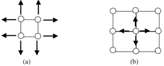
Same in 2IBGSOM, the proposed MIGSOM has three distinct phases. First, the network starts with a rectangular grid of connected nodes (2×2) or (3×3). Second, the structure of the network dynamically increases by adding new nodes. Then, this process can be generated from the node that accumulates the highest quantization error. This unit cannot be only from the boundary, but also from the interior of the network (see Fig. 1). We have to mention that a boundary node can have from one to three free neighboring positions. But, internal nodes do not have free neighboring positions. Therefore, this process can produce multi-levels of maps.

B. Training process of MIGSOM

The MIGSOM training process starts with initialization phase, that we random initiate weight vectors and the Growing Threshold (GT) to control the growth of the map. Then, architecture grows as time passes by adding. Finally, a

smoothing of the map is achieved. During this phase, no new nodes are added. More details of MIGSOM algorithm are presented as follows:

Initialization Phase

1. Start with a random rectangular grid of 4 or 9 connected nodes.

2. Calculate the growth threshold (GT) for the given data, similar to [1] for controlling the growth of the map.

Growing Phase

3. Train the map using all inputs patterns. Identify winners nodes and update weight vectors according to the following learning rule :

(

)

( )

1

1 n

ci j j

i n

ci j

h t x

w t

h t

=

⋅

+ =

∑

(1)

wi(t) refers to the weight vector of unit i,

( )

ci

h t is the neighborhood kernel centered on the BMU (Best Match Unit).

( )

t

(

Ud

)

Ud

t

hci  t −

  

  −

=

σ

1

2 exp ) (

2 2

(2) σ : measures the degree to which excited neurons in the vicinity of the winning neuron cooperate in the learning process.

1(x)=0 if x<0 and 1(x)=1 if x>=0.

Ud is the distance between neurons c and i on the map. 4. Calculate the error of each node and identify the node q

with the highest quantization error.

1

k

j q i

Err x w

=

∑

− (3)

k: the number of units mapped in the node q.

5. If (Errq > GT), then new nodes will be generated from q whether it is a boundary node or not.

6. Initialize the new node weight vectors to match the neighboring node weights.

7. Repeat steps 3)-6) until the number of iterations is reached or to attempt a fixed quantization error.

Smoothing Phase

8. Fixe the neighborhood radius to one.

9. Training the map in the same way as in growing phase without adding new nodes.

C. Insertion process of new node

The insertion process of new node is usually from the unit that accumulates the highest quantization error. Fig. 2 presents the four situations that can occur for adding nodes.

In case (a), if a boundary node is selected for growth, then all its free neighboring positions will be filled with new nodes.

In case (b), if an internal node is selected for growth, then four new nodes are inserted between this node and its four immediate neighbors. This new nodes are added in the superior level of the map.

In case (c) and (d), nodes can be added from the boundary

(a) (b)

(3)

or the interior of the network as in case (a) and (b).

(a) (b)

(c) (d)

Node with high quantization error New nodes

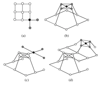
Fig. 2 Insertion of new nodes. (a) From the boundary (b) From the interior (c) From the boundary in the superior level of the map and (d) From the interior in the superior level of the map

D. Weight initialization of new node

Similar in [3], the weight initialization of new added nodes is made to match the weight of neighboring nodes (Fig. 3). New weight depends on the weight of nodes positioned of one of the sides of the node with the highest Error.

The weight initialization in case (a) and (b) is made to Eq. (4) or (5). The difference in two cases is the position of the neighbor. When both cases are available, case (a) is used.

(

2 1

)

1 1

2 W then W W W W

W

if new= − − (4)

(

1 2

)

1 2

1 W then W W W W

W

if new= + − (5)

In case (c) the new node is between two older nodes, then Eq. (6) is used.

(

1 2

)

2 new

W W

W = + (6)

(a) Wnew W1 W2

(b) W1 W2

Wnew

(c) W2 Wnew W1

Fig. 3 Weight initialization of new nodes

Wnew: weight vectors of the new node generated

W1, W2: weights vectors of the two consecutive old nodes

positioned on the sides of the new node.

III. EXPERIMENTAL RESULTS

In this section, we will report some experimental results to demonstrate the performances of our method to well preserve the data topology and quantification compared to

the classical SOM and GG algorithms with same maps size. Then we make to use three datasets: two of them are two-Dimensional synthetic data sets (Dataset 1 and Dataset 2) [2], and the Iris flower data set [7] [4].

A. Map Quality Measures

The accuracy of a map in representing its inputs can be measured with the Average Quantization Error (AQE) [17] and the Topologic Error (TE) [17]. The AQE tests the distortion of the representation for the model. The TE tests if the distribution of the training data maintains the neighborhood relationships between nodes throughout the training process.

Quantization Error

We propose to evaluate our model by the NQE (Normalized Quantization Error) presented by Eq. (7). It is the mean of the Average Quantization Error (AQE) of each node. However, AQE is the average distance between each data vector and its BMU (Best Match Unit) that should be very close. NQE is equal to one; if no data point is match the weight vector of a unit.

( )

 

  

 

   

 

   

 

−

=

∑

= =

unit the match is point data no if

w norm

w x k N NQE

N

j j

k

i

x c

i i

, 1

1 1

) (

(7)

xi is a single data point, N is the number of nodes,

k is the number of data-vector mapped of each unit,

wc(xi) is the weight vector of the Best-Matching Unit in the

map for xi,

. : indicate the Euclidean norm.

Topologic Error (TE)

The Topologic Error is presented by Eq. (8). It tests the neighbor neurons’ relationship. Such that for an input i, if the best matching unit (BMU) and the second BMU are adjacent neurons, then the topology is preserved, else there is a distortion in the map.

N otherwise

r r if

TE

N i

sbi bi

∑

=

> −

= 0 0,

1 ,

1

(8)

N is the number of nodes in the map,

rbi and rsbi are respectively the positions of BMU and second

BMU of input i _{on the map.}

B. Results and discussions

(4)

either a rectangular topology (4 direct neighborhoods) or a hexagonal topology (6 direct neighborhoods). Since, MIGSOM and GG have a rectangular topology the same common parameters are chosen.

In our experiment, the MIGSOM algorithm is trained in two phases. In the growing phase, we use a decaying neighborhood radius rate from 2 to 1. Then, for the smoothing phase, we use a fixed neighborhood radius rate (equal to 1) and only five iterations.

The GG algorithm is trained used the simulation parameters presented in [9] with constant neighborhood range and adaptation strength in growing phase and with decaying adaptation strength in the fine-tuning phase.

The SOM algorithm is trained in the two versions as known in literature. For the sequential training process of SOM, we use the “Gaussian” neighborhood function. In the ordering phase, learning rate α_o_{=0.5 and neighborhood}

radius rate decrease from 2 to 1. In the fine-tuning phase, learning rate α_t_{= 0.05 with time invariant neighborhood of 1.}

For the batch version of SOM, we use “Cutgauss” neighborhood function and a decaying neighborhood radius rate from 2 to 1 same with MIGSOM. Then, the fine-tuning phase is trained with a fixed radius rate to one.

1)Dataset1

For this experimental study, we test three SOMs algorithms against Dataset1 [2]. The data base is a two-Dimensional synthetic data set of 1600 data points that can be distributed in four clusters.

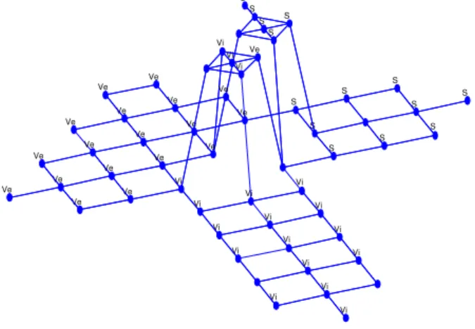
The MIGSOM structure is increasing dynamically. Then, the growing process is along of 50 iterations. As a result, see Fig. 4 and Fig. 5. However, Fig. 4 illustrates the labeled MIGSOM grid structure with 135 connected nodes. As shown the map has irregular structure with multi-levels oriented maps, there is the result of interior growing. Therefore, the MIGSOM grid structure presents homogenous clusters.

Fig. 4 Grid structure of MIGSOM for Dataset 1.

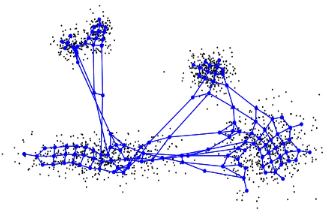
Fig. 5 shows a well topologically ordered MIGSOM. The map is well aligned with data distribution, which has small topographic error.

Fig. 5 MIGSOM topologic map structure trained for Dataset 1.

Fig. 6 illustrates the SOM topologic structure of dataset 1 trained with batch versions. The map size is the same generated by MIGSOM algorithm (135 nodes (15×9)). Although the maps take the form of the data structure in general, Maps present distortion of data topology, there are more nodes not perfectly placed.

Fig. 6 Batch SOM map topologic structure trained for Dataset 1.

Fig. 7 illustrates the GG topologic structure of dataset 1 with almost the map size of MIGSOM and SOM (132 nodes (11×12)). Although the maps present less distortion then batch SOM (Fig. 6), there is more data point that are not covered by the map. Contrary in Fig. 5, the distribution of weight vectors improves topology preservation with less distortion.

Fig. 7 GG topologic map structure trained for Dataset 1.

4 4 4 4 4 4 4 4 1

4 1

1

4 1

4 4 1

4 1 1

4 1

4

4 1 1

4 4 1

4

4 4

4 1

4 4

4 4 4 4

3

4 1

4 4 1

4 3

4 4

4

2 3

4

2 3

4

2 3

4

2 3

3

2 3 3

2

2 3 3

2 3

3

2 3

3

2 3

2 3 3

3 3 3

3 3

3 3 3

3 3

3 3 3 3

(5)

Table I summarizes Quantization and topographic quality of the four SOMs. As seen MIGSOM generate less quantization and topographic error compared to GG and SOM with batch and sequential versions algorithm.

TABLE I

RESULTS SUMMARY FOR DATASET 1

Type of SOM NQE % TE

MIGSOM 5.70 % 0.144

GG 10.92 % 0.200

Batch SOM 12.48 % 0.285

Sequential SOM 12.06 % 0.193

2) Dataset 2

Dataset2 [2] is still a two-Dimensional synthetic data set of 1300 data points distributed in thirteen clusters. We also test the three SOMs with comparable map size and the same parameters previously defined.

Fig. 8 illustrates the labeled MIGSOM grid structure for dataset 2 after 55 iterations of growing process. The generated structure takes 142 connected nodes. So the map has irregular structure with homogenous clusters.

Fig. 8 Grid structure of MIGSOM for Dataset 2.

Fig. 9 MIGSOM topologic map structure trained for Dataset 2.

As seen in see Fig. 9, our proposed Multilevel Interior Growing SOM (MIGSOM) is able to automatically choose appropriate position where to insert new nodes during the growth process leading to the final network.

The Self-Organizing Maps (Fig. 10) with pre-defined structure (11×13) may have difficulties to generally represent data topology. The network has a topologic structure with most distortion. The map is not well aligned with data distribution. Thus, SOMs have high topologic error.

Fig. 10 Batch SOM map topologic structure trained for Dataset 2.

Fig. 11 present GG topologic map structure trained for Dataset 2. The generated structure takes 143 (11×13) connected nodes. Although GG find the map size dynamically, the network presents topologic structure with most distortion.

Fig. 11 GG topologic map structure trained for Dataset 2.

Quantization and topologic quality of Dataset 2 for the four SOMs are summarized in Table II. As seen, MIGSOM still generates less quantization and topologic errors with same map size of GG and SOM.

TABLE II

RESULTS SUMMARY FOR DATASET 2

MIGSOM 5.5 % 0.095

GG 6.1 % 0.232

Batch SOM 9.7 % 0.308

3) Iris Data set

The Iris flower dataset [7] [4] is used many times as the benchmark test data set for classification algorithms. The data base has 150 data points, each point has four-Dimensional (flower, namely petal length, petal width, sepal length and sepal width). Then, the Iris data can be distributed in two or three clusters.

MIGSOM is also trained with Iris data set and the result is presented in Fig. 12. Since the data has only 150 data points, MIGSOM growing process is only a long of 20 iterations. They are sufficient to down data to prototypes.

Since Iris flower data set is a four-Dimensional, it cannot be plotted in two-Dimensional space. Thus, we present only in Fig. 12 the grid structure. Also, the generated map (57

2 2 2 1 2 7 2 1 2 2 1 2 2 2 1 2 7 2 2 1 2 7 2 1 2 7 2 2 3 1 2 7 3 7 3 1 2 7 3 7

1 7 3 1 2

1 7

1 3 3 1 2

1 1 1

1 7

3 3 7

1 1 1

1 7

3 7

4 1 1 1

1 7

7 4 4 1 1

1 9 4 4 1 1 1 9 4 4 1 1 9 4 4 1 1 9

9 4 9

1 1 9

4 9

5 9 9

8 5 5 1 1 8 8 5 1 3 9 8 5 1 3 1 0 8 5 1 3

5 1 3 8 8 1 3

5 1 3 1 0 8 5 1 3 1 0 1 0 6 1 3 1 3 1 0 8 1 3

6 1 3 1 0

6 1 3 1 0 1 0 6 6 1 0

(6)

connected nodes) has irregular structure with multi-levels oriented maps.

Fig.12 Grid structure of MIGSOM for Iris Data set.

Quantization and Topologic Error for Iris data set for four SOMs are summarized in Table III. Even if the Batch version of SOM has less Quantization Error of MIGSOM; MIGSOM shown significantly improvement of topographic quality than others SOMs.

TABLE III

RESULTS SUMMARY FOR IRIS DATA SET

MIGSOM 13.4 % 0.040

GG 22.7 % 0.273

Batch SOM 12.1 % 0.233

IV. CONCLUSION

In this paper, a new dynamic Self-Organizing feature map is presented. The MIGSOM proposed method is able to adapt its size and structure according to the data topology. MIGSOM add nodes where it is necessary from the unit that accumulates the highest quantization Error (whether the unit is a boundary node or not). Therefore, MIGSOM can have three-Dimensional structure with multi-levels oriented maps.

MIGSOM have been tested with synthetic and real data sets. Experiments results of MIGSOMs compared to GG and the classical SOM show improvement of map quality preservation with similar map size to GG and SOM.

Even if GG grow the structure of the network dynamically during the training process, it presents less performance than MIGSOM.

The standard model of SOM with pre-defined structure has difficulties to represent faithfully data topology. However, the MIGSOM network topology preserved well data structure.

Future work can be directed first by decreasing the complexity of MIGSOM through elaborating a specific algorithm. Second by integrate data topology into the visualization of the MIGSOM clusters and thereby providing

a more elaboratedview of the cluster structure than existing schemes.

ACKNOWLEDGMENT

The authors want to acknowledge the financial support of this work by grants from the General Direction of Scientific Research and Technological Renovation (DGRST), Tunisia, under the ARUB program 01/UR/11/02.

REFERENCES

[1] R. Amarasiri, D. Alahakoon, K. A. Smith, HDGSOM: A Modified

Growing Self-Organizing Map for High Dimensional Data Clustering,

Fourth International Conference on Hybrid Intelligent Systems

(HIS'04), 216-221, 2004.

[2] L. D. Alahakoon, S.K. Halgamuge, and B. Sirinivasan, Dynamic Self

Organizing Maps With Controlled Growth for Knowledge Discovery,

IEEE Transactions on Neural Networks, Special Issue on Knowledge

Discovery and Data Mining, 11(3), pp. 601-614, 2000.

[3] T. Ayadi, T. M. Hamdani, M.A. Alimi, M. A. Khabou, 2IBGSOM:

Interior and Irregular Boundaries Growing Self-Organizing Maps,

IEEE Sixth International Conference on Machine Learning and

Applications, 13-15, 2007.

[4] C. L. Blake and C. J. Merz, UCI Repository of machine learning

databases [http://www.ics.uci.edu/~mlearn/MLRepository.html].

Irvine, CA: University of California, Department of Information and Computer Science, 1998.

[5] G. J. Deboeck and T. Kohonen, Visual explorations in finance: with

self-organising maps, Springer, 1998.

[6] M. Ellouze, N. Boujemaa, M.A. Alimi, Scene pathfinder:

unsupervised clustering techniques for movie scenes extraction,

Multimedia Tools And Application, In Press, August 2009.

[7] R.A. Fisher, The use of multiple measure in taxonomic problems,

Ann. Eugenics 7 (Part II) pp. 179–188, 1936.

[8] B. Fritzke, Growing cell structure: A self organizing network for

supervised and un-supervised learning, Neural Networks, vol. 7, pp.

1441–1460, 1994.

[9] B. Fritzke, Growing grid-A self-organizing network with constant

neighborhood range and adaption strength, Neural Processing Lett.,

vol.2 (5), pp. 1-5, 1995.

[10] T. M. Hamdani, M. A. Alimi, and F. Karray, “Enhancing the

Structure and Parameters of the Centers for BBF Fuzzy Neural

Network Classifier Construction Based on Data Structure,” in Proc.

IEEE International Join Conference on Neural Networks, Hong

Kong, pp.3174–3180, June 2008.

[11] A.L. Hsu, S.K. Halgarmuge, Enhanced topology preservation of

Dynamic Self-Organising Maps for data visualization, IFSA World

Congress and 20th NAFIPS International Conference, vol.3, 1786 –

1791, 2001.

[12] M. Kim and R.S. Ramakrishna, New indices for cluster validity

assessment, Pattern Recognition Letters, Vol.26, Issue 15, pp. 2353-2363, 2005.

[13] T. Kohonen, “Statistical Pattern Recognition with Neural Networks:

Benchmark Studies”, Proceedings of the second annual IEEE

International Conference on Neural Networks, Vol. 1.

[14] T. Kohonen, Self Organizing Maps, Third ed. Verlag: Springer, 2001.

[15] T. Kohonen, Self-organization and associative memory.

Springer-Verlag, Berlin, 1984.

[16] J. Vesanto, Using SOM in Data Mining, Licentiate’s Thesis,

Department of Computer Science and Engineering, Helsinki University of Technology, APR 2000.

[17] T. Villmann, M. Herrmann, R. Der and M. Martinetz, “Topology

Preservation in Self-Organising Feature Maps: Exact Definition and

Measurement,” IEEE Transactions on Neural Networks, Vol. 8, No.

2, MAR 1997.

[18] G. Pölzlbauer, A. Rauber, and M. Dittenbach, “Advanced

visualization techniques for self-organizing maps with graph-based

methods,”in Proc. 2nd Int. Symp. Neural Netw., Z. Y. Jun Wang and

X. Liao,Eds., Chongqing, China, pp. 75–80, Jun. 1, 2005.

S

S S S

S

Vi S

Vi Vi S

Vi Vi S S

Vi

Vi S

Vi S Ve S

Vi S

Ve Vi

Vi Vi

Ve Vi

Vi Ve

Ve Ve

Ve

Ve Ve

Ve

Ve Ve