EXPLORATORY GEOSPATIAL DATA
ANALYSIS USING SELF-ORGANIZING MAPS
Case Study of Portuguese Mainland Regions
by
Fernando Correia Lourenço
Dissertation submitted in partial fulfilment of the requirements for the degree of
Mestre em Ciência e Sistemas de Informação Geográfica
[Master in Geographical Information Systems and Science]
Instituto Superior de Estatística e Gestão de Informação
da
ii
EXPLORATORY GEOSPATIAL DATA
ANALYSIS USING SELF-ORGANIZING MAPS
Case Study of Portuguese Mainland Regions
Dissertation supervised by
Professor Doutor Victor José de Almeida e Sousa Lobo
iii
I want to express my appreciation and gratefulness to Victor Lobo, my supervisor, and to
Fernando Bação, that all the way has been like a supervisor to me, for their helpful advice
and support provided for this thesis. I also would like to thank to Pedro Cabral for his wise
iv
SELF-ORGANIZING MAPS
Case Study of Portuguese Mainland Regions
ABSTRACT
The rapidly increasing volume of digital geographic data is overwhelming for conventional
analysis techniques and methods. Therefore new approaches are needed to transform
data into information, and ultimately, into knowledge. Exploratory data analysis is a
foundation stone in this process. It is concerned with the formation of a simplified
overview of data sets. Clustering and projection are among the examples of useful
methods to achieve this task. The Self-Organizing Map (SOM) algorithm performs both, in
a non-linear mapping from a high-dimensional data space to a low-dimensional space
aiming to preserve the topological relations in the data.
The aim of this thesis is to demonstrate the effectiveness of SOM application in visual
exploration of physical geography data to support the delineation of Portuguese mainland
regions. The main justifications for the application of SOM in this issue are its features of
stressing local factors and topological ordering. For experimental assessment, the public
domain thematic maps from Instituto do Ambiente are used. Several authors’ maps of
Portuguese regions are used for evaluation of empirical results.
Categorical attributes found in the data set are problematic in the SOM algorithm. One
way to tackle them is to convert them into binary attributes. For the task at hand,
Euclidean distance and unconstrained real-valued codebook patterns are shown
empirically as suitable approaches to deal with these binary attributes.
The distinctive character of geospatial data and the discrete nature of the SOM are
important issues that should be taken into consideration. In this respect, adequate
geospatial unfolding of SOM is presumed to assist a better representation of geographic
phenomena. Some approaches to assist this objective are put forward and experimented
such as weighting attributes and samples, and a SOM variant named Geo-SOM. Some
visualization methods to address the information extraction issue are also suggested.
Notwithstanding the vagueness of geographic phenomena, experimental results reveal
v
USANDO MAPAS AUTO-ORGANIZÁVEIS
Aplicação ao Estudo das Regiões de Portugal Continental
RESUMO
A crescente quantidade de dados geográficos em formato digital é avassaladora para os
métodos e técnicas de análise tradicionais. Daí a necessidade de novas abordagens para
transformar os dados em informação e, em última análise, em conhecimento. A análise
exploratória de dados é uma peça fundamental neste processo onde se procura obter
uma representação simplificada dos dados. Exemplos de métodos úteis para atingir este
objectivo são o agrupamento e projecção. O algoritmo Mapa Auto-Organizável (SOM)
realiza ambos num mapeamento não linear dum espaço de elevada dimensão para um
espaço de reduzida dimensão tentando preservar as relações topológicas nos dados.
Pretende-se nesta tese demonstrar a eficácia da aplicação do algoritmo SOM na análise
exploratória de dados de geografia física para apoio à delimitação das regiões de
Portugal continental. As principais justificações para a aplicação do SOM neste caso são
a sua ênfase nos factores locais e a sua ordenação topológica. Na demonstração
experimental recorrer-se-á a dados do Instituto do Ambiente. Os resultados empíricos
serão confrontados com mapas de regiões portuguesas de diversos autores.
Os atributos categóricos nos dados usados levantam alguns problemas no algoritmo
SOM. Para lidar com estes pode-se convertê-los em atributos binários. No caso actual,
mostra-se empiricamente que o uso da distância euclidiana e de modelos reais são
abordagens apropriadas para os atributos binários.
O carácter distinto dos dados geo-espaciais e a natureza discreta do SOM são tópicos
que devem ser considerados. Neste aspecto, presume-se que um adequado desdobrar
geo-espacial do SOM contribui para uma melhor representação dos fenómenos
geográficos. Diversas abordagens neste sentido são apresentadas e experimentadas
como a ponderação de atributos e de amostras, e variantes do SOM. São também
sugeridos métodos de visualização para lidar com a questão da extracção da informação.
Apesar do carácter difuso dos fenómenos geográficos, os resultados experimentais
revelam padrões consistentes com os mapas de referência das regiões de Portugal
vi Geographical Information Systems (GIS)
Exploratory Data Analysis (EDA)
Self-Organizing Maps (SOM)
Geospatial Data
Visualization
PALAVRAS-CHAVE
Sistemas de Informação Geográfica (SIG)
Análise Exploratória de Dados
Mapas Auto-Organizáveis
Dados Geo-espaciais
vii
AI Artificial Intelligence
BMU Best Matching Unit
DM Data Mining
EDA Exploratory Data Analysis
GIS Geographical Information Systems (Science)
KDD Knowledge Discovery from Databases
MAUP Modifiable Areal Unit Problem
MDS Multidimensional Scaling
PCA Principal Component Analysis
SOM Self-Organizing Map, Kohonen Map
viii
x variable, attribute or feature (scalar or categorical)
x vector, pattern, data object
i
x
component i of vector x (variable or attribute)i
m
model, reference, or codebook vector of neuron or unit ici
h
kernel neighborhood functionix
ACKNOWLEDGMENTS... iii
ABSTRACT ... iv
RESUMO... v
KEYWORDS ... vi
PALAVRAS-CHAVE... vi
ABBREVIATIONS AND ACRONYMS... vii
NOTATIONS AND CONVENTIONS ...viii
LIST OF TABLES ... xii
LIST OF FIGURES...xiii
1. Introduction ...1
1.1 Background ...1
1.2 Aim of this Study ...3
1.3 Scope and Issues Dealt in this Study ...4
1.4 How this Thesis is organized ...5
2. Searching for Natural Regions in Physical Geography ...7
2.1 Physical Geography...8
2.1.1 Portuguese Mainland Regions ...9
2.2 Selected Data Set ...13
2.3 Data Cleaning and Preparation ...14
2.4 Data Preprocessing ...16
2.4.1 Data Normalization ...17
2.4.2 Data Set Reduction ...17
2.5 Exploratory Data Analysis...18
2.5.1 Clustering and Projection Algorithms ...18
2.5.2 K-means and Davies-Bouldin Index ...19
2.6 SOM Algorithm...20
2.6.1 Introduction to SOM...20
2.6.2 Interpretation of the SOM ...23
x
2.7.1 Geospatial Data Idiosyncrasies...25
2.7.2 Discrete Nature of SOM ...26
2.7.3 SOM Training: Initialization and Parameter Selection...27
2.8 Contributions for the Application of SOM to Geospatial Data...27
3. Dealing with Categorical Data in SOM ...30
3.1 Binary-based Similarity Measures for Categorical Data and Application in SOM 30 3.1.1 Data Types and their Measures ...30
3.1.2 Classification Based on the Domain Size and Measurement Scale ...31
3.1.3 Measures of Distance and Similarity ...32
3.1.4 Categorical Data...33
3.1.5 Similarity Measures ...34
3.1.5.1 Simple Matching ...34
3.1.5.2 Tanimioto ...34
3.1.5.3 Hamming...34
3.1.5.4 Other Similarity Measures ...35
3.1.6 Choice of Similarity Measure for Binary Data ...37
3.2 Benchmark Example...38
3.3 Clustering Binary Data With SOM ...40
3.3.1 Problems in using SOM for Binary Data...40
3.3.2 Proposed SOM architecture ...40
3.3.3 Experimental Results...41
3.3.3.1 Using Euclidean Distance...41
3.3.3.2 Using “hard” logic...42
3.3.3.3 Using “Dot Product” Approach...44
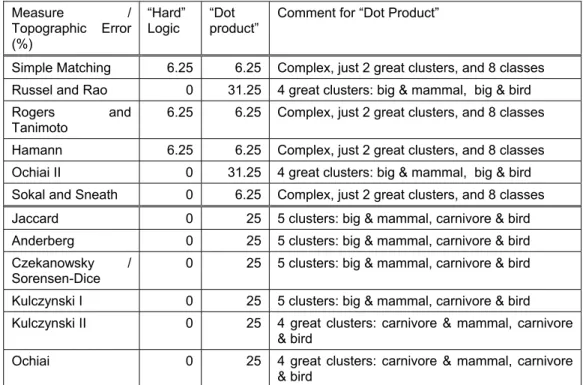
3.3.4 Analysis of Results ...46
3.4 Conclusions from Experiments With Binary-based Similarity Measures...46
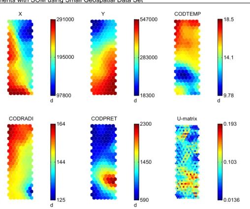
4. Experiments with SOM using a Small Geospatial Data Set ...48
4.1 Linear Initialization without Location Attributes...49
4.2 Linear initialization and use of location attributes ...52
4.3 Geo-initialization ...55
4.3.1 Without Maintaining Geospatial Aspect...55
4.3.2 Maintaining Geospatial Aspect...56
xi
4.5 Standard SOM with Sample Weighting by Area Value...64
4.6 Geo-SOM ...68
4.7 Discussion of Experiments with Small Geospatial Data Set...73
4.7.1 Data Processing and SOM training ...73
4.7.2 Visualization and Information Extraction ...73
4.7.3 Patterns revealed ...74
5. Experiments with SOM using the Final Geospatial Data Set ...75
5.1 Standard SOM using Sample Weighting ...75
5.2 Geo-SOM ...80
5.3 Summary of Experiments and Quality Measures ...84
5.4 A Regions Map Sketch ...85
6. Discussion...87
6.1 Methods ...87
6.2 Exploratory Data Analysis...88
6.3 Interpretation of the SOM...89
7. Conclusions...91
7.1 Conclusion ...91
7.2 Recommendations for Further Work...92
References ...94
A. Appendices ...101
A.1 Source Thematic Maps ...101
A.2 Metadata of Source Maps...102
A.3 Matlab M-files for Similarity Measures...105
xii
Table 2.1 - Summary of geographic phenomena and features on mainland Portugal ...10
Table 2.2 - Themes used in the geospatial data set. ...14
Table 3.1 - Contingency table values...35
Table 3.2 - Similarity coefficients considering negative co-occurrence (Meyer, 2002)...36
Table 3.3 - Similarity coefficients not considering negative co-occurrence (Meyer, 2002)37 Table 3.4 - Animals Data Set ...38
Table 3.5 - Some similarity values ...39
Table 3.6 - Identical maps obtained using real to binary conversion...44
Table 3.7 - Identical maps obtained using “dot product” approach...44
Table 3.8 - Comparison of topographic errors and clustering for similarity measures ...46
Table 5.1 - Summary of most relevant experiments. ...84
xiii
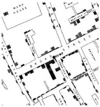
Figure 1.1 - Snow’s cholera map detail showing contaminated well and fatalities as short
lines (Frerichs, 2000). ...1
Figure 2.1 - Regions Maps of Gomes and Girão (Caldas and Loureiro, 1966) ...11
Figure 2.2 - Regions Maps of Lautensach and Ribeiro (Caldas and Loureiro, 1966) ...12
Figure 2.3 - Regions Map of Albuquerque (Caldas and Loureiro, 1966) ...12
Figure 2.4 - Example of map mismatch ...14
Figure 2.5 - Geospatial distribution of centroids for small data set (left) and final data set (right)...16
Figure 2.6 - Effect of independent normalization ...17
Figure 2.7 - Example of SOM grid folding for a input pattern, marked X (Vesanto, 1997). ...22
Figure 2.8 - Data samples: polygon centroids (left) or extra random points (right). ...26
Figure 3.1 - U-mat using Euclidean measure. ...42
Figure 3.2 – U-mat for Simple Match measure. ...43
Figure 3.3 - U-mat for Rao measure. ...43
Figure 3.4 - U-mat for Ochiai II measure ...43
Figure 3.5 - U-mat for Simple Match measure...45
Figure 3.6 - U-mat for Russel and Rao measure ...45
Figure 3.7 - U-mat for Jaccard measure ...45
Figure 3.8 - U-mat for Kulczynsky II measure...45
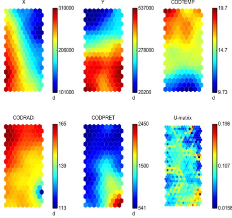
Figure 4.1 - U-mat and component planes with linear initialization and without location attributes ...50
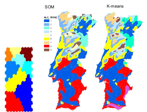
Figure 4.2 – Clustering on rotated U-mat (left) and regions maps using SOM (center) and k-means (9 regions, right) with linear initialization and without location attributes. ....51
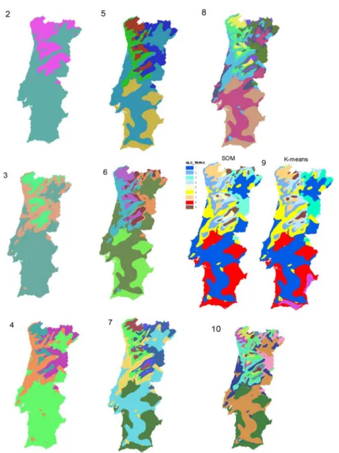
Figure 4.3 - Clustering sequence with linear initialization and without location attributes (nr. of clusters on top left of each map). ...52
Figure 4.4 - U-mat and component planes with linear initialization and location attributes. ...53
Figure 4.5 - Regions on rotated U-mat (left) and map (right) using k-means (10 regions) with linear initialization and location attributes...54
Figure 4.6 – Twisted SOM grid on location plane. ...54
Figure 4.7 - U-mat and component planes with geo-initialization. ...55
xiv
geospatial aspect. ...57
Figure 4.10 - Rotated U-mat and map for best clustering (2 regions) with geo-initialization maintaining geospatial aspect. ...57
Figure 4.11 - Rotated U-mat and map for second best clustering with geo-initialization maintaining spatial aspect...58
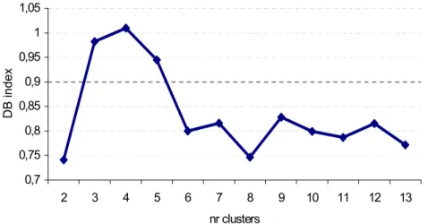
Figure 4.12 – Evolution of the Davies-Bouldin index (DB) as a function of the number of clusters...58
Figure 4.13 - Clustering sequence with geo-initialization maintaining geospatial aspect (2 clusters top left, 9 clusters bottom right) ...59
Figure 4.14 - Standard SOM grid on location plane; effect of final radius (1, left, 0.1 right) ...60
Figure 4.15 - Standard SOM: maps of U-mat accounting all components (left) and excluding location (right). Underlying maps of Gomes and Albuquerque, respectively (Caldas and Loureiro, 1966). ...61
Figure 4.16- SOM grid (left), maps of U-mat values with all components (center) and without location (right) for increased location weight. Background regions of Lautensach and Albuquerque, respectively (Caldas and Loureiro, 1966)...62
Figure 4.17 - Component planes and U-mat for fixed location of codebook vectors...63
Figure 4.18 - SOM grid on location plane for fixed location of codebook vectors. ...63
Figure 4.19 - Component planes and U-mat for SOM full range sample weighting ...65
Figure 4.20 - Component planes and U-mat for SOM with sample weighting with area (range 1-101). ...65
Figure 4.21 - SOM grid on location plane for area weighted data samples (range 1-101). U-mat with (left) and without (right) location components. ...66
Figure 4.22 - Standard SOM: maps of U-mat with all components (left) and without location (right) for weighted data samples (range 1-101). Background regions of Albuquerque and Lautensach, respectively (Caldas and Loureiro, 1966)...67
Figure 4.23 - Standard SOM: maps of U-mat with all components (left) and without location (right) for weighted data samples (full area value). Background maps of Gomes and Albuquerque, respectively (Caldas and Loureiro, 1966)...68
Figure 4.24 - Component planes and U-mat for Geo-SOM, k=1 ...69
Figure 4.25 - Geo-SOM: maps of U-mat using radius k=0, 1 and 3 (respectively from left to right), for small data set. Background maps of Gomes, Girão and Lautensach, respectively (Caldas and Loureiro, 1966). ...70
xv
data set. ...72
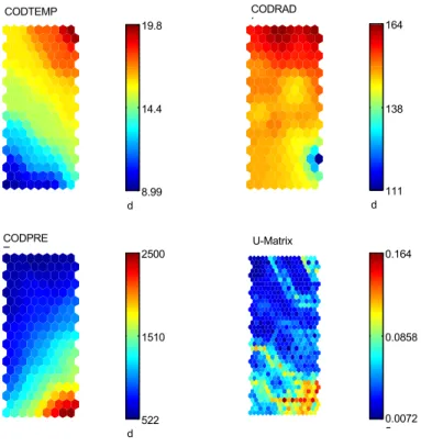
Figure 5.1 - First six component planes and U-mat for standard SOM, full range sample weighting (final data set). ...76
Figure 5.2 - Standard SOM: rotated U-mat (left) and grid (right) on location plane for full-weighted data samples (final data set). Labels identify SOM units. Some regions are pointed out. ...77
Figure 5.3 - Standard SOM grid on location plane for full-weighted data samples (final data set, left) and k-means best Davies-Bouldin index clustering (11 regions, right).78 Figure 5.4 - Maps of U-mat for standard SOM with all components (left) and without location (right) for full-weighted data samples (final data set). Background maps of Gomes and Lautensach, respectively (Caldas and Loureiro, 1966). ...79
Figure 5.5 - Map detail of standard SOM with areas labeled with their BMU number...80
Figure 5.6 - First six component planes and U-mat for Geo-SOM (final data set). ...81
Figure 5.7 - Regions on rotated U-mat for Geo-SOM (final data set). ...81
Figure 5.8 - Geo-SOM grid on location, final data set, (left) and k-means best partition for Davies-Bouldin index (right)...82
Figure 5.9 - Geo-SOM: U-mat values with all components (left) and without location (right), final data set; background regions of Lautensach and Ribeiro, respectively (Caldas and Loureiro, 1966). ...83
Figure 5.10 - Sketch of a possible delineation for the Portuguese mainland regions based on experiments with Geo-SOM and final data set. ...86
1. Introduction
Exploratory data analysis can
never be the whole story, but
nothing else can serve as the
foundation stone - as the first step
(Tukey, 1977).
1.1 Background
In the 1850s, the English physician John Snow performed a pioneering geographic data
analysis to support his hypothesis that cholera was spread in the drinking water (e.g.
Goodchild and Kemp, 1990; Frerichs, 2000). To illustrate his findings he plotted cholera
fatalities and pumps on a map (detail shown in Figure 1.1) where he was able to show
that cholera deaths had clustered around a particular pump (Frerichs, 2000).
His arguments led to the decision to remove the well pump, putting an end to that source
of epidemic. Though associations between phenomena are usually harder to detect, this
case is a very simple one.
However, the rapidly increasing volume, dimensionality and the complexity of digital
geographic data overwhelm conventional analysis techniques and methods (Openshaw,
1993; Fayyad, Piatetsky-Shapiro and Smyth, 1996; Gahegan, 1996; Miller and Han,
2001). Here most traditional statistical methods are not adequate because of their high
computational burden or very restrictive assumptions on data (Openshaw, 1993;
Chambers et al., 1998; Fayyad, Grinstein and Wierse, 2002). Thus they are generally
unsuitable for geographic data analysis largely due to spatial dependency and complexity
of geographic phenomena (e.g. Longley et al., 2001; Miller and Han, 2001).
Therefore new approaches are needed to transform data into information, and ultimately,
into knowledge (Fayyad, Piatetsky-Shapiro and Smyth, 1996; Openshaw and Openshaw,
1997; Miller and Han, 2001). New ideas may by inspired in new computing tools that are
essentially data driven rather than theory driven, and applied rather than theoretical in
their motivation (Openshaw, 1993).
Data Mining (DM), Knowledge Discovery in Databases (KDD) and Artificial Intelligence
(AI) bring important contributions to this issue (Miller and Han, 2001). Neural networks
have been revealed in recent years as an interesting and promising field (e.g. Openshaw
and Openshaw, 1997). However, a shortcoming of neural networks is the difficulty to
extract information embedded therein (e.g. Openshaw and Openshaw, 1997).
As one of the first steps in the knowledge discovery process, Exploratory Data Analysis
(EDA) addresses data not yet understood, classified, summarized or unstructured and
most of its techniques are graphical in nature (Tukey, 1977; Tufte, 1998a; Tufte, 1998b).
They greatly rely on the one of the most sophisticated information processing system: the
human eye-brain visual system (Chambers et al., 1998). Visualization of geographic data
(geographic visualization or geo-visualization in computer systems) thus can leverage
human experts’ capabilities on pattern recognition, in a rich environment for formulating
hypothesis, theory, and explanations (e.g. Gahegan, 2001; Worboys and Duckham,
2004). In fact, maps are effective tools for presenting geospatial data because they
provide abstract graphical model of the world (e.g. Worboys and Duckham, 2004).
To enable the discovery or identification of features or patterns of most relevance there is
a need for data reduction and projection. Clustering and projection are amongst the
a grouping of data according to a chosen criterion (Hair et al., 1998). Projection methods,
on the other hand, represent the data points in a lower dimensional space in such a way
that the clusters and the metric relations of the data items are preserved as faithfully as
possible (Hair et al., 1998).
In this thesis a type of neural network, the Self-Organizing Maps (SOM), is used to
perform data clustering and projection. It has been applied in a large variety of tasks, such
as pattern recognition, image analysis, data analysis, voice recognition, process control
and optimization (Kohonen, 2001). The SOM algorithm resembles vector quantization
algorithms. The major distinction between the SOM and other vector quantization
techniques is that in the former the units are organized on a regular grid and along with
the selected unit its neighbors are also updated, yielding an ordering of the units
(Kohonen, 2001). The algorithm performs a non-linear mapping from a high-dimensional
data space to a low-dimensional space, typically two-dimensional, rectangular grid
(Kohonen, 2001). This allows the presentation of multidimensional data in two
dimensions, assisting the visual exploration of data. As the SOM compresses data while
preserving the most important topological relationships it may be thought as producing
some kind of abstractions (Kohonen, 2001).
Several proposals and studies for the delineation of geographic regions on mainland
Portugal have been undertaken (Girão, 1933; Albuquerque, 1945; Caldas and Loureiro,
1966; Ribeiro, 1987; Gaspar, 1993). Their objective is achieved, basically, in a clustering
scheme trying to find regions characterized by internal homogeneity while maximizing
heterogeneity between regions (e.g. Longley et al., 2001). Nowadays, wide-ranging and
public domain data are available that can be used for this purpose. This puts a challenge
and an opportunity to take advantage of that asset in order to enhance the understanding
of our country. The type of data and its dimensionality also suggests the application of
new approaches in GIS.
1.2 Aim of this Study
The aim of this study is to demonstrate the effectiveness of SOM algorithm in the task of
exploring geospatial data, in the search for interesting patterns in physical geography of
Portuguese mainland. Ultimately, to seek empirical evidence or relations with regions as
The following SOM properties, which will be discussed later, make it most useful to this
purpose:
• Data Reduction
o Projection of data in a 2-D grid (map metaphor)
o Clustering
• Local factors analysis;
• Topology preservation.
1.3 Scope and Issues Dealt in this Study
This study is focused on exploratory geospatial data analysis with SOM. It emphasizes
what is special about geospatial data that needs consideration for SOM application, and
methods to extract and present information from SOM output.
In fact, categorical attributes and the character of geospatial data give rise to some issues
on its application in SOM. A shortcoming of SOM is also the difficulty of extracting
information from it. Several approaches to tackle these issues are studied, proposed and
evaluated, notably:
• Choices of similarity measure in BMU selection and subsequent effects in SOM clustering.
• Enforce SOM geospatial unfolding
• Visualization aids to picture SOM unfolding.
• Convert 2-D source data (polygons) into 0-D (points) as required for input by SOM algorithm.
• Present the SOM output on geographic maps of U-mat as groundwork for exploratory analysis.
For the first topic, a binary data set of animal features (Ritter and Kohonen, 1989) is used
geospatial data set based on thematic maps from mainland Portugal (Instituto do
Ambiente, 2003) and maps of regions proposed by several authors make up the basis for
experimental assessment of the core of this study.
Ideally, the target SOM clustering should yield connected regions, i.e. there should be no
enclaves (or islands). Actually, it is a challenge to embed this objective in SOM mapping,
yet this matter is not tackled in the current study.
The exploratory data analysis pursued within the current study is neither meant to be
exhaustive nor self-contained. Indeed, there are so many degrees of freedom and
expanding possibilities in this process that it is not possible to cover them all here.
Moreover, this also makes it impractical to benchmark all methods and identify the most
suitable, which is also not proposed here.
1.4 How this Thesis is organized
Chapter 1 draws the background and motivation for this study, and outlines its scope. The
thesis statement is established here.
Chapter 2 begins with an introduction to the framework of this thesis and experiments,
with an outline of the Knowledge Discovery in Databases process. Then it proceeds with
literature review about Physical Geography and Portuguese mainland regions for domain
knowledge. The topics of data selection and data processing are brought in along with
discussion pertinent to the data set used in this study. Exploratory data analysis and SOM
algorithm are described briefly. Thereafter, an overview is made about what makes
geospatial phenomena and data distinctive when compared with most non-georeferenced
data. Along these sections, details and discussions relevant to this study are introduced.
The major contributions of the current study are presented at the end of this chapter.
In Chapter 3 is presented a classification of data types and an overview of similarity
measures for patterns. It focuses on categorical variables; implications and approaches to
deal with them in SOM are presented.
In Chapters 4 and 5, the empirical results are presented for exploratory geospatial data
analysis using standard SOM and a variant (Geo-SOM). In the former chapter, a small
data set is used and in the later the whole, final data set, is introduced. An outline of a
framework for geospatial data analysis using SOM is also suggested. Ultimately, an effort
In Chapter 6, an overall discussion about experiments is brought forward.
In Chapter 7 is presented an overall evaluation of the experiments. Here the conclusions
with respect to the validity of the statement are drawn. Recommendations for future work
2. Searching for Natural Regions in
Physical Geography
The main goal of this study is to explore geospatial data using SOM in order to search for
interesting patterns in geospatial data from mainland Portugal. This task can be suitably
incorporated into the broader perspective of knowledge discovery process.
A comprehensive definition for knowledge discovery in databases (KDD) as stated by Fayyad, Piatetsky-Shapiro and Smyth (1996) is “the non-trivial process of identifying valid, novel, potentially useful and ultimately understandable patterns in data”. We can outline the process of KDD in the following phases (Fayyad, Piatetsky-Shapiro and Smyth, 1996):
• Domain knowledge and Goal Definition
• Data Set Selection
• Data Cleaning and preprocessing - Empty values analysis
- Conversion of data types (numerical and categorical)
- Invalid data analysis
- Data normalization
• Data Set Reduction and Projection
• Matching the goals of the KDD process
• Exploratory Analysis
• Data Mining
• Interpreting the mined patterns
• Action!
Although the focus of this thesis is on exploratory data analysis, this outline provides a
thorough framework for the study. It is noteworthy that, generally, this process is not as
These topics and the herewith case study also illustrate the interdisciplinary nature of
Geographical Information Systems and Geographical Information Science (GIS). A
comprehensive view of GIS is that of a field dealing with geospatial data and phenomena.
It is built on the knowledge of geography, cartography, mathematics, computer science,
engineering and many other areas of science (Peuquet and Marble, 1991; Wright,
Goodchild and Proctor, 1997; Heywood, Cornelius and Carver, 1998; Painho and Peixoto,
2002; Worboys and Duckham, 2004). The term geospatial is used along this study to mean geographically referenced (e.g. Worboys and Duckham, 2004). Therefore,
geospatial data is a special type of data that relates to the surface of the Earth.
Next, we introduce some literature review useful for domain knowledge, an introduction to
SOM algorithm and some discussion about what makes geospatial data distinctive.
Approaches to enable a geospatial unfolding of SOM and methods to extract information
from SOM are also presented.
2.1 Physical Geography
A good knowledge of the phenomena involved will be of great value in the selection, and
preparation of the input data (e.g. Bação, 2002). Hence, we present an overview of
concepts and literature about these subjects.
Physical Geography can be described as the branch of Geography (e.g. Small and Witherick, 1992) that, amongst other features, studies:
• the surface shape of the Earth (Geomorphology);
• rivers, lakes, and underground water (Hydrology);
• seas, and oceans (Oceanography);
• atmospheric processes and phenomena (Climatology and Meteorology);
• soil types and their formation (Pedology);
• distribution of plants and animals (Biogeography)
Unlike those features studied in Human Geography, these are related to energy
transformations in which man does not have a major role (e.g. Jones, 1985). However,
exclusion of some themes, like vegetation, from the geospatial data set to be used in the
current study because they have been deeply influenced by human activities
(Albuquerque, 1945).
2.1.1 Portuguese Mainland Regions
A region is a territory whose distinctive features or a set of criteria, grants it unity and differentiates it from neighborhood land (e.g. Jones, 1985; Small and Witherick, 1992).
These are the main topics of regional geography which is fundamentally concerned with the delineation of zones characterized by internal homogeneity (uniform regions) while
maximizing heterogeneity between zones (e.g. Longley et al., 2001).
As stated before, human interaction often has great influence on environment. Some
authors also account for the human factor. For instance, for Ribeiro (1987) a natural region is a harmonious space with character, emanating from a long adjustment of generations to the environment that they, in great part, shaped. In this thesis, however, a
natural region will have a more restrictive interpretation because only physical factors are
considered thus excluding human factors. Consequently, the resulting regions should
essentially reflect physical geographic phenomena.
One of the most ancient types of region, or spatial organization, in Portugal is the
Concelho whose origin is prior to the birth of the nation (Saraiva, 1978). The Província is
a larger region that represents a traditional space, with a more historic than functional
substance (Caldas and Loureiro, 1966) – a reminiscence of former administrative regions.
Inspired by the French revolution, the províncias were abolished and, instead, another
region was created: Distrito. This is done joining several concelhos with a diversity of
conditions (e.g. Girão, 1933). There are many other regions that we could refer but with
much less importance, like ecclesiastic, judicial, agricultural, or forest regions.
In a survey about Portuguese geography (Girão, 1933; Albuquerque, 1945; Birot, 1950;
Caldas and Loureiro, 1966; Ribeiro, Lautensach and Daveau, 1987; Selecções do
Reader's Digest, 1988; Medeiros, 1991), we may get a picture of the most important
geographic phenomena and features that characterize this country. These are
Land relief and structure
The more notorious and greatest geologic regions are Hesperic Massif, Mesozoic borders, Tertiary basin of Tagus and Sado rivers. In this subject, we must refer tectonic and volcanic processes (stable areas, faults and seismic accidents) - endogenic forces that create the relief, and exogenic forces (such as erosion) that shape it. These have a contribution on the geologic evolution of rock and soil types. Mainland plate has a general slope to west on the northern territory and to southwest on the southern territory, reflected on the course of the major rivers, as Douro, Tagus and Guadiana (Ribeiro, Lautensach and Daveau, 1987).
Geographic position
The most important factors are latitude, location in mainland, and elevation
Atmospheric dynamics
Solar radiation is a major factor, but air circulation, temperature, summer and winter precipitation distribution, cloudiness, frost, impacts in watercourses, soil and vegetation, altogether characterize climate (Medeiros, 1991). The Atlantic Ocean exerts deep influence on climate (fading from seaside to interior) and also does the Mediterranean Sea (greater on south) (Ribeiro, Lautensach and Daveau, 1987).
Table 2.1 - Summary of geographic phenomena and features on mainland Portugal
Several authors have elaborated geographic divisions based on some or most of these
factors. The following lines give an overview of the main topics presented by those
authors.
• Barros Gomes for his 1878 map relies essentially on latitude, exposition and relief (Caldas and Loureiro, 1966).
• Girão (1933) pays attention to the human factor.
• Hermann Lautensach for his map of 1932 (Caldas and Loureiro, 1966), being geomorphologist, bases his division essentially on relief and soil structure.
• Ribeiro, Lautensach and Daveau (1987) consider climate, position, soil, relief, vegetation, and also human influence.
• Albuquerque (1945) considers essentially ecological factors: soil, climate, and vegetation. In this last factor, he just considers forests of native species,
because they would be less subject to human activities. He remarks the
relevance of Geology and Orography.
• Caldas and Loureiro (1966) are responsible for one of the first methodic investigations on delimitation of homogeneous regions, taking into account
ecological and human factors (social and economical). By means of factorial
analysis, their elementary regions (concelhos) are clustered in a way that
• Gaspar (1993) builds the regions based on the distritos, and thus is essentially inspired on administrative limits without great other methodic substance.
• Birot (1950) has one of the simplest delineation’s, encompassing all northern regions in just one region, and then considers Estremadura, Ribatejo, Alentejo,
and Algarve.
From Figure 2.1 through Figure 2.3 the maps of selected authors are shown (Caldas and
Loureiro, 1966). The delineation of Caldas and Loureiro (1966) and Gaspar (1993) will not
be considered. The former because it emphasis human factors and the later because it is
based only on previous administrative limits.
Gomes Girão
Lautensach Ribeiro
Figure 2.2 - Regions Maps of Lautensach and Ribeiro (Caldas and Loureiro, 1966)
Albuquerque
These maps will be used as references in order to evaluate the experimental results.
They will also be overlaid to most of the maps presented in this study.
2.2 Selected Data Set
The source for the geospatial data set is the public domain “Atlas do Ambiente” (Instituto
do Ambiente, 2003), dated April 21, 2001. The maps are released in shape format with
military coordinate system and Lisbon Datum. Although interesting, a thorough analysis of
the data set is beyond the scope of this thesis. Furthermore, in order to show our points in
exploratory data analysis, we are interested in maintaining data complexity and volume to
a reasonable amount (e.g. Mitchell, 1997).
In the previous section, the groundwork was established for a preliminary theme selection
whereupon we elect six themes that we consider the most relevant to this study:
elevation, hydrographic basins, lithology, precipitation, solar radiation, and temperature
(Table 2.2). There we indicate which themes (bold) and fields are used in our
experiments. Some will be used only as reference or background (tagged Ref). Maps
showing a qualitative or quantitative property (theme) are usually described as thematic maps (e.g. Burrough, 1990; Tufte, 1998b). In Appendix A.1, the thematic maps of the geospatial data set used in this study are shown. Further details about these maps are
also included in Appendix A.2.
Taking into account the two geographic coordinates (location), the selected data set has a
dimensionality of eight instead of 47 (the dimensionality of the whole data set from “Atlas
do Ambiente”). The proposed reduced dimension of data is advantageous by reducing
Theme shp name used Use field type Comments
Elevation cniv2 Yes GRIDCODE scalar polyline theme converted to polygon
Hydrographic basins
baci Yes CODBACI categorical major river basins
Lithology
litosin Yes CODLIT categorical sedimentary, sedimentary
and metamorphic, plutonic eruptive
Precipitation pret Yes CODPRET ratio annual mean
Solar radiation radi Yes CODRADI ratio annual mean
Temperature temp Yes TEMPERATUR scalar annual mean
Concelhos con Ref boundaries
Mainland limit lim_simp Ref country boundary
Concelho name topo_c Ref label
Natural regions regi Ref REGIAO as in Albuquerque (1945)
Table 2.2 - Themes used in the geospatial data set.
2.3 Data Cleaning and Preparation
A common problem when dealing with data from several sources is their variable
accuracy or lack of spatial consistency (Burrough, 1990). This is mostly noted at map
borders where maps do not overlap completely. An example, extracted from the
geospatial data set used in this study, can be seen in Figure 2.4. It introduces the issue of
dealing with missing values at map borders. In these cases, the approach in the current
study is a pragmatic one, discarding regions with missing values.
Figure 2.4 - Example of map mismatch
In order to produce the data set in the required tabular format for the SOM, the thematic
obtain many areas also named polygon features in GIS software. We assume that all locations inside an area will have identical values for all attributes.
Spatial intersection requires that the input themes must have polygon topology (area).
Unfortunately, source elevation theme has an additional shortcoming: it is a polyline
(linear) theme. It has many contour lines that are open or intersect somehow each other.
This makes impossible automatic use of procedures to create valid topological polygons.
The huge amount of data in this theme also would make a formidable task doing that
correction manually. Hence, we had to envisage a practical approach to overcome this
issue. Our option was to recreate a 3-D surface model using the contour elevation data.
This operation will eventually introduce some error that, is hoped, will not affect
significantly the experiments.
The 3-D surface was built using ArcMap 3-D Analyst, creating a TIN from contour lines.
Then we recreated closed contour lines from the TIN. In general, this procedure smoothes
the original contour lines, many of which are, indeed, very convoluted. Though introducing
error, this may be useful in reducing data amount, notably the number of small regions we
have to process.
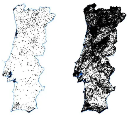
Two geospatial data sets are thus set up, a simpler one, called hereafter small data set, having temperature, solar radiation and precipitation, and another, called hereafter final data set, joining elevation, hydrographic basins and lithology to the former data set. The geospatial distribution of data samples (polygon centroids) for both data sets is shown in
Figure 2.5 - Geospatial distribution of centroids for small data set (left) and final data set (right).
The SOM algorithm is founded on discrete, 0-D geometry (Silva and Rodrigues, 1983)
points (input and codebook patterns). Here is worth a note in geometry to say that a n -dimensional object is, essentially, one that requires n parameters to describe a location within it. The data at our disposal are mostly polygon (2-D geometry) themes that are a
result of several interpolation methods. Therefore, to be used in the SOM we have to
convert them again to discrete points. Our option is to use the polygon centroid. In a way,
it would be an advantage if we could use the original survey and discrete data samples for
input eventually avoiding some interpolation issues introduced in the released data set.
2.4 Data Preprocessing
Data preprocessing and normalization is generally an unsettled issue. Here we
emphasize the discussion on the geospatial character of the data set used in this study
2.4.1 Data Normalization
When dealing with geospatial data we should take into account its distinctive nature in the
data-preprocessing step. Nevertheless, in most normalization tasks each variable is
treated independently, including location components (x and y). In the current study we
refer to location as the 2-D variable representing geographic position defined by attributes (coordinates) x and y. Therefore, being a 2-D variable, its components should not be treated separately. In Figure 2.6 we illustrate this issue with a very simple example of a
originally circular cluster in a rectangular data distribution (left, dashed circle), a linear
range normalization (center, ellipse) and processing algorithm (center, circle), and the
output after normalization (right, ellipse). As can be seen, when applying the
de-normalization the resulting clusters are squeezed along the variable formerly with the
lower range.
Figure 2.6 - Effect of independent normalization
In this study we will apply a linear scaling to all variables (min-max transformation) so they
are mapped into the [0,1] interval (e.g. Bação, 2002). Furthermore, we propose that
location variables (x and y) should be jointly normalized in order to preserve geospatial
aspect. In the experiments ahead, this is done scaling down the variable x by the ratio
max(x)/max(y). In doing so, it is also presumed that both variables have similar relevance.
2.4.2 Data Set Reduction
Some preliminary correlation analysis or other method could give some help in discarding
less significant variables thus ensuing data set reduction. However, this is out of the
scope of this study. Instead, the choice of variables is based mainly on the literature
2.5 Exploratory Data Analysis
Exploratory Data Analysis (EDA) addresses data not yet understood, classified,
summarized or unstructured (Tukey, 1977). Much like KDD, it aims to uncover interesting
structures or patterns in large data sets and provide some means of explaining it (Fayyad,
Piatetsky-Shapiro and Smyth, 1996). In one of the first works to explicitly use the term
Exploratory Data Analysis (Tukey, 1977) this process is, in fact, envisaged as a detective
work. Because it is free for many constraints it may lack some objectivity, but this may
also be an advantage in data exploration and hypothesis generation (e.g. Gahegan,
2001).
Most Exploratory Data Analysis techniques are graphical in nature, using pictures to
describe data (Chambers et al., 1998; Tufte, 1998a; Tufte, 1998b). They greatly rely on
the one of the most sophisticated information processing system: the human eye-brain
visual system (e.g. Chambers et al., 1998). An example of an advantage of using the
visual domain is that of a picture: it can make large data sets much more accessible than
an extensive list of numbers (Tufte, 1998a; Tufte, 1998b; Gahegan, 2001). In fact, the
primary goal of data visualization is finding a view or projection of the data that reduces
complexity while capturing important information, i.e., reducing complexity while losing the
least amount of information (Fayyad, Grinstein and Wierse, 2002). Here we clearly want
to emphasis the fundamental components in this process. One is the visual presentation
and the other is the human expert, a key player, by his ability to identify patterns (e.g.
Gahegan, 1996).
Traditional measures or tools like minimum, maximum, mean, median, standard deviation,
correlation, plots, histograms, scatter plots, etc. may give us some insight about a data
set (Murteira, 1993; Chambers et al., 1998). But for high dimensional data they may be
ineffective and therefore we need additional tools such as clustering and projection
algorithms (Hair et al., 1998).
2.5.1 Clustering and Projection Algorithms
Classical clustering algorithms produce a grouping of the data according to a chosen
criterion. For instance, minimizing within cluster variance while maximizing between
cluster variance (Hair et al., 1998). As examples, we can refer the following algorithms
which work reasonably well for large geographical databases: partitioning methods
based methods (DBSCAN, OPTICS), and grid methods (STING, CLIQUE) (Gahegan,
2001).
Projection methods, on the other hand, represent the data points in a lower dimensional
space in such a way that the clusters and the metric relations of the data items are
preserved as faithfully as possible (Hair et al., 1998). The data sets can thus be visualized
if a small dimensionality (one to three) is chosen for the output display. Linear projection,
multidimensional scaling (MDS) (Hair et al., 1998), and principal curves are examples of
projection methods (Hastie and Stuetzle, 1989). A brief description of these methods
should be useful in introducing the SOM algorithm and therefore will be given ahead.
Principal components describe the global distribution of the data in terms of linear
combinations of the original variables or, equivalently, linear projections to straight lines in
the data space. The first principal component is defined as the projection of the data to
the line for which as much of the variance of the data is preserved as possible. The
second principal component is the projection to the line that is orthogonal to the first one
and preserves the remaining variance maximally, and so on (Hair et al., 1998).
Multidimensional scaling (MDS) is a class of methods (e.g. Sammon’s mapping) applying
non-linear projections to data that are high dimensional and highly asymmetric to make
possible visualization on a low dimension display (Hair et al., 1998).
Principal curves are generalizations of the principal components, defined to be smooth
curves that go through the center of the data (Hastie and Stuetzle, 1989). Each point of
the curve is the average of all data points projecting to it. The principal curves and
surfaces are closely related to the SOM. A discretized principal surface, together with a
certain kind of smoothing, would be essentially a SOM (Kaski, Nikkila and Kohonen,
2000).
2.5.2 K-means and Davies-Bouldin Index
The SOM alone is not amenable to extensive data mining or feature extraction. For this
reason, further processing of the SOM is needed. Several methods can be applied, such
as k-means clustering or U-mat, described further ahead.
In some experiments of this study, k-means clustering is applied to the SOM. This
procedure is included in SOM Toolbox for Matlab (Vesanto et al., 2000; Helsinki
the k-means is run multiple times and the best partition is selected based on the sum of
squared errors. Afterwards, the Davies-Bouldin index is calculated for each clustering.
This index is rather a guideline for the best partition than an absolute truth (e.g. Siponen
et al., 2001). This method favors spherical compact clusters that are widely separated.
Performing this clustering over the SOM instead of the data directly is, for the task at
hand, a computationally effective approach (Vesanto and Alhoniemi, 2000).
The Davies-Bouldin index chooses the best partition the one that minimizes the
expression:
∑
=
+
C
i
ij j i j
M
S
S
C
1max
1
Where C is the number of clusters,
S
i is the dispersion of cluster i (e.g. mean squared distance from center), andM
ij is the distance between centers of clusters i and j(Siponen et al., 2001).
2.6 SOM Algorithm
2.6.1 Introduction to SOM
The Self-Organizing Maps (SOM) algorithm, also called the Kohonen network, the self-organizing feature map (SOFM) or the topological map, is an unsupervised neural network algorithm developed by the Finish physicist Teuvo Kohonen (2001). It has
biological background on nervous systems (Kohonen, 2001).
It provides two useful operations in exploratory data analysis: clustering, reducing the
amount of data into representative categories, and non-linear projection, aiding in the
exploration of proximity relations in the data (Kaski and Kohonen, 1996). The SOM
algorithm has some resemblance with vector quantization algorithms, like k-means, and is
closely related to principal curves (Kohonen, 2001). The great distinction from other
vector quantization techniques is that the units are organized on a regular grid and along
with the selected unit also its neighbors are updated. As a result, the SOM performs an
mapped also to nearby units in output space. In this respect, the SOM is a
multidimensional scaling method, which projects data from input space to a lower
dimensional output space.
A comprehensive introduction and description of the SOM algorithm can be found in
Kohonen (2001). Here we will just make a brief presentation. The SOM consists of an
array or lattice of elements called neurons or units, usually arranged in a low dimensionality grid (1-D or 2-D), the map, for ease of visualization. The lattice type may have several forms like rectangular, hexagonal or even irregular. Associated with each
unit there is a pattern called model, codebook or reference, having the same dimensionality of the input patterns. The image of an input pattern x on the SOM array is the unit
m
cthat best matches with x. We also call this winning unit the best matching unit(BMU) or winner unit. Using a dissimilarity measure d(x,
m
i), this unit has the index:c=arg
min
i{d(x,m
i)}On the original incremental SOM algorithm, the codebook patterns are updated iteratively
in the learning phase following the rule:
i
m
(t+1)=m
i(t)+α(t)h
ci(t) [x(t)-m
i(t)]In this process
h
ci(t) represents a kernel neighborhood function over the lattice (radius), generally wide in the beginning and decreasing in time, defining which units and howmuch will they be affected by each input pattern and α(t) is the learning rate that also should decrease with time.
A variant of the SOM, besides other differences from the original, works in batch mode
where the whole training set (all input patterns) is gone through at once, and only after
this, the map is updated with the net effect of all the patterns. The updating is done
replacing the codebook pattern with a weighted average over the input patterns:
i
m
(t+1)=∑
∑
= =
n
j ic j n
j ic j j
t
h
t
h
1 ( ) 1 ( )
)
(
)
Where c(j) is the BMU of input pattern xj, hi,c(j) the neighborhood function, and n is the number of input patterns (Vesanto et al., 2000). The weighting factors are the
neighborhood function values.
The codebook patterns are thus updated to follow the input patterns in an ordered way
(an example is shown in Figure 2.7). As a result of this algorithm, the codebook patterns
of close by units should be similar thus preserving most of the topology relations of the
input patterns on the map. We may picture this like an elastic network becoming smoothly
fitted to the input pattern distribution.
Figure 2.7 - Example of SOM grid folding for a input pattern, marked X (Vesanto, 1997).
With due care, we observe some resemblance between the projection properties of SOM
algorithm and of the principal component analysis (PCA). The main difference is the
nonlinear projection of the SOM that can be a great advantage in many cases (e.g.
Verleysen, 1997), like revealing local or fine details. In contrast to PCA, in SOM local
factors impact locally and there they will have greater importance in the projection
In summary, among the several features making the SOM a useful method in Exploratory
Data Analysis we can refer:
• Ordered dimensionality reduction
• Follows data distribution
• Easily explainable and simple
• Easy visualization.
The visualization of complex multidimensional data is one of the main application areas of
the SOM (e.g. Vesanto, 1999). In fact, the SOM has not been made for statistical pattern
analysis; it is a clustering, visualization, and abstraction method (Kohonen, 2001). The
SOM algorithm has been used in a whole wide range of applications such as pattern
recognition, data compression, process optimization (for instance, traveling-salesman
problem), process control (Kohonen, 2001)
2.6.2 Interpretation of the SOM
Information extraction is usually a bottleneck in neural networks (Ultsch et al., 1993;
Openshaw and Openshaw, 1997), and this is no exception in SOM.
As explained earlier, local factors have great impact on SOM algorithm. Therefore, the
interpretation of the SOM output must be analyzed with a focus on local relations.
Extending the analysis to relations that are more global must be done with caution.
Calibrating the SOM map, i.e. locating the images of input patterns on the map and
assigning the labels to some winner units, may be helpful to find relations and patterns in
data (Kohonen, 2001).
The unified distance matrix methods, U-matrix (U-mat) (Ultsch et al., 1993), are a
graphical representation of the SOM map structure and provide us very useful assistance.
In the simplest of these methods for each codebook pattern the mean of the dissimilarity
measures to its neighbors is computed. Plotting this data on a 2-D map, using a gray or
color scheme, we can visualize a landscape with walls (mountains) and valleys (plains). The walls separate different classes, and patterns in the same valleys are similar (Ultsch
color scheme we can envisage the regions because areas close to each other on the
U-mat will have similar colors (e.g. Vesanto, 1999).
The U-mat and component planes (where the contribution of each variable is shown) are
very useful for visual analysis (Kaski, Nikkila and Kohonen, 2000) mainly when they can
be easily related, for example by sharing a common coordinate system (Kaski and
Kohonen, 1998).
Some approaches to automate the interpretation of SOM apply additional clustering to the
SOM, using classical partitioning methods, for example with k-means and Davies-Bouldin
index for evaluation, as explained earlier (Siponen et al., 2001), or hierarchical (Vesanto
and Alhoniemi, 2000). Other approaches try to evaluate some common features of
several nearby codebook units and using them for automatic labeling (Rauber, 1999).
Displaying the number of hits in each SOM unit may also be used where units with low
number of hits suggest cluster borders (Kaski, Nikkila and Kohonen, 2000).
In some experimental results of this study, a further clustering by the k-means algorithm is
applied to the SOM. However because k-means generally does not unveil fine details,
here is further proposed a geographic map of U-mat, with richer detail, and a colored
SOM grid, both based on U-mat methods.
2.6.3 SOM Algorithm Complexity
The complexity of the SOM incremental algorithm (and k-means algorithm) is O(n·d·k·m), where m is the number of epochs, n the number of data samples, d is the data dimension,
k is number of map units (or clusters in k-means). It is mostly determined by the number of epochs m and data samples n (Strehl, Ghosh and Mooney, 2000). If n>>m the complexity of “batch training” is half of sequential training (Vesanto et al., 2000), thus
making it a more practical choice for experimental purposes.
2.7 Application of SOM to Geospatial Data
When modeling geospatial data in SOM several issues and techniques (such as biasing
the training phase of the SOM) might introduce detrimental effects on the final output.
Here the usual measures for SOM quality assessment like quantization or topographic
errors (Kaski and Lagus, 1996; Vesanto et al., 2000; Kohonen, 2001) may be not we
effective quality of the SOM obtained will persist. Though deserving real care, this
discussion is beyond the scope of this thesis.
2.7.1 Geospatial Data Idiosyncrasies
Geospatial data are characterized by information about position or location, connections
with other entities and details of non-spatial characteristics (Burrough, 1990). Besides
these, geospatial data have some other unique features when compared with most
non-geographic data. One of them is their spatial dependency, the tendency of attributes at
some locations in space to be related (e.g. Wong, 1996; Miller and Han, 2001). It is
similar to dependency in other domains but is, generally, more complex. On the other
hand, contributing for the amazing richness and diversity of geography is spatial
heterogeneity. This refers to the non-stationarity of most geographic phenomena (e.g.
Miller and Han, 2001). Each place has its own uniqueness. This is why estimated global
parameters may not describe adequately geographic phenomena at any particular
location (e.g. Miller and Han, 2001).
Another distinctive aspect is the complexity of geographic phenomena (e.g. Goodchild
and Kemp, 1990). Most non-geographic data can be easily represented with discrete
points without losing important properties. However, this is not the case for most
geographic phenomena where, for example, size, shape, boundaries, direction, and
connectivity cannot be properly represented by simple points or lines (e.g. Miller and Han,
2001). Furthermore, observations of geographic phenomena are intrinsically imperfect
due to error, imprecision and vagueness (Duckham et al., 2001; Longley et al., 2001;
Worboys and Duckham, 2004). There is a geospatial variation due to the fundamental
aspect of nature that occurs at all scales, also perceived by its gradual, fuzzy or vague
changes (Burrough, 1990). These explain the inexistence of crisp boundaries for most
geographic phenomena.
The geospatial data set used in this study additionally suffers from errors introduced with
discretization, interpolation and classification methods (Burrough, 1990). The former has
to do with the limited resolution of observations and representation of real world
phenomena (e.g. Worboys and Duckham, 2004). The later introduces issues of several
spatial scales and different surface partitioning that are related to the commonly known
modifiable areal unit problem (MAUP) (Openshaw, 1984). For instance, choosing other
2.7.2 Discrete Nature of SOM
On a fine enough scale of resolution all geographic phenomena are discontinuous (e.g.
Griffith and Layne, 1999). However, on coarser scales of resolution, as those dealt in this
study, those phenomena can appear to be continuous. However, SOM as a quantization
algorithm, tries to adjust a discrete manifold to a discrete data distribution. In fact, the
SOM algorithm is basically conceived to deal with 0-D geometry objects - points. These
are characterized by a position in space, but no length (e.g. Goodchild and Kemp, 1990).
However, the objects represented by the source data set have a 2-D geometry. To
somehow overcome this issue we have to sample the input space in order to obtain the
required discrete input data for SOM. Consequently, each 2-D polygon will be
represented by its centroid (a 0-D point). An example is shown in Figure 2.8 (left). This
artificial 0-D point reference provides a summary of the location of the object (e.g. Longley
et al., 2001). A shortcoming of this procedure is that we drop valuable topological
relations in the data such as size, shape, and neighborhood (Miller and Han, 2001). To
compensate this loss, at least somewhat, we propose to weight the data points with their
corresponding area values (source polygons). Another choice could be to devise a more
even geospatial sample density, for instance, generating random extra data samples,
mostly in larger areas. An example is shown in Figure 2.8 (right). These areas would,
consequently, get a more balanced representation in SOM. Though more accurate, a
major drawback of this procedure would be of greatly enlarging the data set and,
consequently, introducing a heavy computational burden.
2.7.3 SOM Training: Initialization and Parameter Selection
Common approaches to the initialization of the codebook pattern may use an initial state
that is ordered or arbitrary; for example, use linear spanning along the main eigenvectors
of the data auto-correlation matrix (PCA) or use random values (Kohonen, 2001). The
former, generally, provides better and faster results (Kohonen, 2001). However, in this
study, we are more interested in a geographic point of view, and thus we will use the
geo-initialization of SOM. This is achieved spanning the SOM grid (codebook patterns)
regularly along the geospatial rectangle defined by data location attributes (coordinates x
and y), and other components are drawn from the geographically nearest neighbor.
The SOM training phase also must enable a geospatial unfolding of SOM grid. This may
be done in the process of BMU evaluation by means of suitable location weighting. This
entails essentially an empirical (trial) approach. For example, if we introduce a location
weight too high the SOM grid is compelled to follow essentially the geographic data
(density) distribution. On the other hand, if the location weighting is too low, other
non-geographic measures may prevail and the pursued geospatial unfolding is not
accomplished. In-between there are many possibilities and therefore location weighting
must be sensibly adjusted in order avoid these problems and achieve a geo-enforcing of
the SOM. These may be evaluated inspecting the SOM grid on the location plane.
Another important issue is how to obtain a small number of regions (about 10) as
presented in the literature review or how much detail should be revealed. One approach
would be choosing an adequate map size, noting that a map with fewer units will also
allow fewer clusters and, thus, will be simpler to inspect. Another possibility is to use the
empirical rule of thumb that suggests 5
n
units for the map, where n is the number of data samples (Vesanto et al., 2000). In our first experiments, using the smaller data set,we defined our map size with that rule and, where possible, we will keep it unchanged.
2.8 Contributions for the Application of SOM
to Geospatial Data
Several approaches for the application of SOM algorithm to geospatial data were
presented and suggested beforehand such as data preprocessing (normalization,
attribute and sample weighting) and geo-initialization (Bação, Lobo and Painho, in press).
perspective also led to the deployment of methods that are suggested here. These are
useful to visualize the unfolding of SOM and extract information from it, both from a
geospatial viewpoint. In fact, it would be interesting if we could envisage the SOM
somehow as a conventional geographical map, thus making full use of the map metaphor
(Old, 2002; Skupin, 2003; Worboys and Duckham, 2004). With this ideas in mind, a
suggestion is made to project the SOM grid onto the location plane (input subspace). This
will show how the SOM unfolds geospatially. Furthermore, to harness the potential of the
map metaphor, the geographic map of U-mat is introduced here. This map may assist, at
the first glance, the exploratory geospatial analysis.
In the colored SOM grids, the size of nodes (units) and the color of the connections
depend on their U-mat values. The width of SOM grid connections is also made
proportional to their U-mat values. Finally, to give the geospatial perspective, we project
the SOM grid into location coordinates (input subspace), thus immediately revealing the
SOM geospatial unfolding. This makes up another important tool to evaluate the SOM
initialization and training.
To explore the results in a geographic map, we have to convert the discrete output of
SOM to a space analogous to the original input space. In this matter, instead of
generating Thiessen polygons (Bação, Lobo and Painho, 2004), in this study a simple
classification of data samples (areas) is proposed based on their BMU. This association,
between data samples and their BMU, suggests interesting and simple ways of visualizing
patterns in SOM. For instance, creating a thematic map based on some meaningful and
distinctive attribute of the BMU. At this point, the U-mat value computed at the node (the
BMU) was considered and that showed up to be the most revealing. Therefore, we
present several maps where each area is colored according to the U-mat value of its
corresponding BMU.
The rationale behind the maps of U-mat is the assumption that the SOM grid must have a
smooth and comprehensive geospatial unfolding. The U-mat values shown are those
computed at the lattice node and give information about similarity between codebook
vectors (output space). It is assumed that SOM unfolding preserves most topologic
relations in the input data. Therefore, it can be expected that those U-mat values will give
a suitable representation of geospatial relations in input data due to the geo-enforcing of
In interpreting these maps, the following rules are very important:
• Exploratory analysis on the map must be done locally.
• Nearby areas with similar colors are likely to be similar and thus belong to the same region
• Color itself reveals how much a region is similar to surrounding areas.
Relations with specific surrounding areas (units) must be investigated through the SOM
grid or U-mat. It must be stressed that the proposed coloring scheme with U-mat must be
interpreted for local patterns rather than global ones. A global interpretation can be
achieved projecting the SOM into a color space (Kaski, Venna and Kohonen, 2000) or
k-means clustering of SOM (Vesanto and Alhoniemi, 2000). In these cases, a more
extensive analysis may be done though at the expense of missing local and fine detailed
patterns.
Throughout this study the mat, component planes, k-means clustering and maps of
U-mat will be used to present the experimental results. These visualization aids provide
useful insight into geography. Moreover, joining input data, codebook vectors and U-mat
on the GIS software, a whole range of interactive exploratory analysis is feasible, like