Fiscal strategic interaction in Brazil: An
analysis of Fiscal War of Ports
Enlin on M
o
*F i n Ro h
†João M l f Júnio
‡Contents: 1. Introduction; 2. Brazilian State Tax System; 3. Empirical strategy; 4. Data; 5. Estimation results; 6. Conclusion; Appendix.
Keywords: Fiscal War of Ports, Strategic Behavior, States. JEL Code: H2, H7.
The purpose of this paper is to evaluate a particular competitive interaction among Brazil-ian states, the Fiscal War of Ports (FWP) and to verify if Resolution 13/2012, which reduced the tax rate on imported goods in interstate sales, had the desired impact. Using monthly data on state importing levels during the period from January 2010 to April 2015 we find evidence that Brazilian states do engage in spatial interaction, and that Resolution 13/2012 has changed the spatial interaction among states since 2013 and more deeply in the beginning of 2014.
O objetivo deste trabalho é avaliar a eventual interação competitiva entre os estados bra-sileiros, a Guerra Fiscal de Portos (FWP) e verificar se a Resolução 13/2012, que reduziu a alíquota sobre bens importados nas vendas interestaduais, teve o impacto desejado. Usando dados mensais sobre os níveis de importação do estado no período de janeiro de 2010 a abril de 2015, encontramos evidências de que os estados brasileiros se envolvem na intera-ção espacial e que a R13 mudou a interaintera-ção espacial entre os estados desde 2013 e mais profundamente no início de 2014.
1. INTRODUCTION
Fiscal competition models usually assume that jurisdictions finance the provision of public goods with taxes on local capital. Capital is nationally fixed, but can easily move to other jurisdictions in response to tax-rate differentials, while labor is typically immobile.
There are two versions of these models. According to the competitive version, jurisdictions are small relative to the economy and thus are unable to affect the net-of-tax return to capital. As a result, tax rates in other jurisdictions are irrelevant, and strategic behavior is absent. According to the strategic version, each jurisdiction is large relative to the economy and therefore is able to affect the net return of capital changing its own tax rate. The tax rates in other jurisdictions must be taken into account in a given jurisdiction’s choice, leading to strategic behavior.
*Escola de Economia de São Paulo, Fundação Getúlio Vargas (EESP/FGV). Rua Itapeva 474, 13º andar, Bela Vista, São Paulo, SP. CEP 01332-000. Email:Enlinson.mattos@fgv.br
†Universidade de São Paulo. Email:frocha@usp.br
Brazilian states and municipalities have been engaging over the years in strong tax competition, known as “fiscal war”. The impact of tax competition, however, has not been empirically tested and most of the evidence is informal. It indicates no impact on real activity and mainly the erosion the tax base. There are few exceptions though. Mello(2007) estimates a tax reaction for Brazilian states in the period 1985–2001 and finds evidence that states react to changes in their neighbours’s VAT rates, existing even a Stackelberg leader.Nascimento(2008), uses a differences-in-differences approach to compare São Paulo (a state which did not engage in fiscal war) to the other states. He concludes that the fiscal war has not significantly changed the employment rate of the industrial sector or the tax revenues. Regarding local governments,Barcellos(2004), using micro-data, shows that two cities around the city of São Paulo were able to use changes in their municipal taxes to attract firms to their territories, but with no corresponding increase in the number of jobs.1
The purpose of this paper is to evaluate a particular competitive interaction among Brazilian states, the Fiscal War of Ports (FWP). Under the Fiscal War of Ports special tax regimes took the form of tax credits over interstate sales of imported goods. In order to apply for these special tax regimes, firms need only to change the original port through which they import their goods to the port of the conceding state. Sales tax over importing goods operations that would be owed to the state of the original port are then collected by the conceding state, which earns the difference between the tax revenue collected and credit tax benefit conceded. The original state, on the other hand, loses all tax revenue from that operation, and firms earn the tax benefit, paying less sales tax eventually.
We intend to test for the existence of strategic interaction among states due to the Fiscal War of Ports and also to evaluate if Resolution 13/2012 (R13), which reduced the tax rate on imported goods in interstate sales, had the desired impact.
The paper is organized in five sections besides this introduction. Insection 2 we present an overview of the Brazilian state tax system, especially regarding the interstate sales taxation and the FWP working process. Insection 3, we present the econometric strategy. Insection 4we present the data and insection 5we discuss the regression results. Insection 6we summarize the main conclusions.
2. BRAZILIAN STATE TAX SYSTEM
2.1. Understanding the ICMS
The main tax charged by the Brazilian states and the Federal District is a consumer tax named ICMS (Imposto sobre a Circulação de Mercadorias e Serviços). It has two rates, one for transactions that occur inside the state and other for interstate transactions.
For example, São Paulo state’s internal flat tax rate over the majority of operations is 18%. In interstate operations though, the tax rate depends on both the state of origin and the state of destination of the goods and services. In operations between two states from the richest regions (like São Paulo and Minas Gerais), the interstate tax rate is 12%, and in operations between a state from a rich region and a state from a poor region, it is 7%. Therefore, São Paulo collects 7% of tax over the imposing base and the state at poor region collects the remaining 11% of tax over the same imposing base. The main idea is to split tax revenues in favor of the poorer region.
1Regarding the international literature, there is a well established strand of economists, such asBesley & Case(1995),Figlio,
ICMS is a non-cumulative type of taxation. The tax rate is applied over the invoice face value of the acquisition and paid by the selling company, whereas the purchasing company registers the same value paid by the selling company, as a credit in its ICMS assessment accounts.
When the former purchasing company sells the same product it will apply the tax rate over its selling price, which will be presumably higher than the acquisition price, giving that it made a profit. Since the tax is non-cumulative this company pays an amount correspondent to the total amount of tax calculated in the sales operation minus the value appropriated as a credit in the ICMS assessment account, which is exactly the amount of tax calculated in the precedent acquisition.
In other words, the amount o ICMS levied is equal to the tax value paid in the acquisition plus the tax rate over the value added (profits) in its current operation. At the end of the day, the company will pay ICMS only over the value that it has added, avoiding double counting.
In the firms’ accounting books will appear a credit, a value of ICMS that such firm has the legal right to appropriate, corresponding exactly to the tax paid in the former sales, and a debit, a value of ICMS that such firm has the legal obligation to pay, corresponding to the tax owed by such firm due to the subsequent sale of the same goods. The balance debit vs. credit will result, in a monthly basis, in the net amount that will be owed and effectively paid by the firm to the State authority.
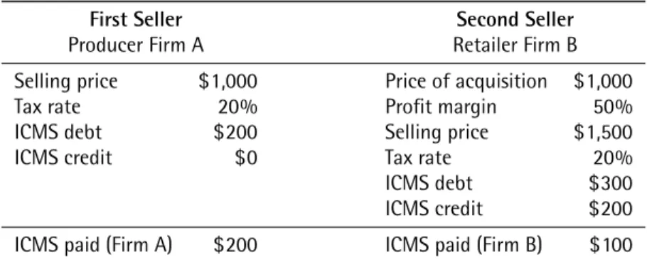
Table 1brings an example of two firms, a producer, Firm A, and a retailer, firm B, located at the same state X, trading one particular type of good over which the ICMS tax rate is equal, lets’ say, to 20%.2 We assume for simplicity that Firm A has no ICMS credit because, for instance, it didn’t have to
buy any raw materials or supplies for its production process. Conversely, firm B has an ICMS credit of US$200 which corresponds to Firm A’s ICMS debit. Both firms pay 20% of ICMS over their sale prices.
At the end of this two firm’s chain the total amount of ICMS paid will be $300. Firm A paid $200, and firm B paid $100. Eventually, the amount o ICMS firm B pays corresponds exactly to an incidence of ICMS solely over the value it added to the trade chain.
Table 1. Non-cumulative principle – internal operation.
First Seller Second Seller
Producer Firm A Retailer Firm B
Selling price $1,000 Price of acquisition $1,000
Tax rate 20% Profit margin 50%
ICMS debt $200 Selling price $1,500
ICMS credit $0 Tax rate 20%
ICMS debt $300
ICMS credit $200
ICMS paid (Firm A) $200 ICMS paid (Firm B) $100
2.2. The Fiscal War of Ports
The Fiscal War of Ports (FWP) can be defined as a competition among Brazilian states to attract invest-ments to their territories by means of fiscal incentives to either Brazilian or foreign trading companies if they do their importing operations through the conceding state harbors.
The ICMS non-cumulative principle makes the concession of tax benefits easy. They can assume the form of an ICMS credit or the form of a reduction or deferral of tax due which impacts the debit account.
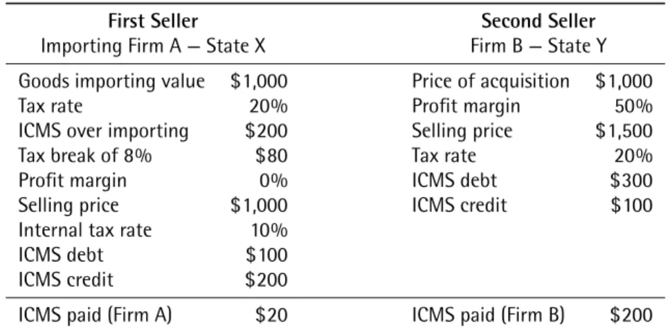
A numerical example can help to understand FWP’s working mechanism. Tables2,3and4show two trading firms, Firm A selling to firm B, in three different situations. InTable 2, none of the firms receive tax benefit and both firms are located in the same state. InTable 3, there is also no tax benefit, but firms are located in different states. Finally, inTable 4, firms are located in different states and Firm A gets a tax benefit (direct concession of ICMS credits over interstate sales of imported goods).
For the sake of simplicity, we consider that both the internal tax rates and the tax rate on the importing operation are 20% and that the interstate tax rate is 10%. We also assume, with no loss of generality, that Firm A has zero profit.
Table 2shows that Firm A pays to State Y an amount of $200 corresponding to ICMS over the importing operation, plus the amount of $200 corresponding to the ICMS over the internal operation, minus the amount of $200 corresponding to the ICMS paid over the import operation trade, or $200 ( + − ).
Firm B, on the other hand, pays to State Y an amount of $300 corresponding to the ICMS over its sales minus an amount of $200 corresponding to the amount paid by Firm A due to the non-cumulative principle, or $100.
At the end of the day, State Y gets a tax revenue of $300, corresponding to $200 paid by Firm A and $100 paid by Firm B.
Table 3shows that Firm A, located at State X, pays to State X the amount of $200 (ICMS over the importing operation), plus the amount of $100 (ICMS over the interstate operation) minus the amount of $200 (ICMS paid over the importing operation), or $100 ( + − ). Firm B, located at State Y, which buys the imported goods from Firm A, located at State X, pays $200 to the State Y.
Therefore, State X gets $100 and State Y gets $200 as tax revenues. Indeed, due to the interstate operation tax revenues are split between the two states.
When we compare the situations inTable 2andTable 3, it is possible to see that the two states share the tax revenue generated in the interstate but only State Y all the internal sale tax revenues belong to State Y. Then, States have incentives to attract importing firms to their territories not only to promote economic development, but mainly to grab part of the tax revenues generated in sales operations.
Suppose that both Firm A and firm B are located at State Y, but now State X is willing to attract Firm A to its territory in order to grab part of the tax revenues generated by firm’s A sales to firm B, as inTable 3. In order to do that, State X concedes a tax benefit to Firm A corresponding to a credit of ICMS of 8% over the value of the imported good (Table 4).
State Y receives the same amount of tax revenues as before, but it receives less than he used to receive when Firm A was located in State Y. State Y, therefore, loses revenues as a consequence of the benefit conceded by State X.
State X will receive tax revenues of only $20. This small value corresponds to the amount of $100 that Firm A would originally pay of taxes in an interstate sale, minus the amount of $80 of ICMS tax privilege. On the other hand, Firm A will pay less ICMS due to the direct credit of $80.
Indeed, if we compareTable 2and4we can see that State X increases its tax revenues from zero to $20. Firm A pays less ICMS and State Y loses part of its ICMS revenues (a decrease from $300 to $200).3
Table 2. Non-cumulative principle – internal operation.
First Seller Second Seller
Importing Firm A — State Y Firm B — State Y
Goods importing value $1,000 Price of acquisition $1,000
Tax Rate 20% Profit margin 50%
ICMS over importing $200 Selling price $1,500
Tax rate 20%
Profit margin 0% ICMS debt $300
Selling price $1,000 ICMS credit $200
Internal tax rate 20%
ICMS debt $200
ICMS credit $200
ICMS paid (Firm A) $200 ICMS paid (Firm B) $100
Table 3.FWP – interstate operation without tax break.
First Seller Second Seller
Importing Firm A — State X Firm B — State Y
Goods importing value $1,000 Price of acquisition $1,000
Tax rate 20% Profit margin 50%
ICMS over importing $200 Selling price $1,500
Tax rate 20%
Profit margin 0% ICMS debt $300
Selling price $1,000 ICMS credit $100
Interstate tax rate 10%
ICMS debt $100
ICMS credit $200
ICMS paid (Firm A) $100 ICMS paid (Firm B) $200
Table 4.FWP – interstate operation with tax break.
First Seller Second Seller
Importing Firm A — State X Firm B — State Y
Goods importing value $1,000 Price of acquisition $1,000
Tax rate 20% Profit margin 50%
ICMS over importing $200 Selling price $1,500
Tax break of 8% $80 Tax rate 20%
Profit margin 0% ICMS debt $300
Selling price $1,000 ICMS credit $100
Internal tax rate 10%
ICMS debt $100
ICMS credit $200
FWP is in most of the cases just a commercial type of fiscal war and as such features no capital inversions. Since firms gain rents and do not have to invest, they will be constrained to move to another state only if the operational costs involved are higher than the benefits received.
Due to the increase in the benefits offered, in the beginning of 2013, the Congress passed Senate Resolution 13 (R13). The purpose of R13 is to decrease the tax rate applied over imported products in interstate sales in order to diminish the amount of tax revenues that these operations generate for the states, and the profits that firms could extract in the form of tax benefits. The ultimate purpose was to control the Fiscal War of Ports by reducing the willingness of firms to accept the special tax regimes.
Suppose that the original interstate tax rate is 10%, and after R13 that tax rate is only 4%. The states conceding tax benefits of 8% will not to be able to continue do so. In fact, 4% becomes the maximum rate that states could give as benefits.
3. EMPIRICAL STRATEGY
Brueckner(2003) presents an overview of the empirical models of strategic interactions among gov-ernments and a review of the econometric issues involved in the estimation of reaction functions. He classifies the empirical studies in two broad categories: spillover models (yardstick and environmental models), and resource-flow models (tax competition and welfare competition models).4
In spillover models each jurisdiction� chooses the level of a decision variable�� and is directly
affected by the level of �−� chosen by the others jurisdictions, yielding a reaction function of the
type�� = �(�−�;��), where �� is a vector of jurisdiction� characteristics. In resource-flow models, a
jurisdiction is not affected directly by the level of the decision variable� of others jurisdictions, but by a particular resource within its borders, such as the level of imports or the number of importing companies. However, the reaction functions in these models end up being exactly the same as the ones in the spillover models given that the distribution of that particular resource also depends on the level of�and of characteristics�of each jurisdiction.
Since both types of models yield the same type of reaction function, researchers face a hard identification problem. AsBrueckner(2003) states, it is not possible to know the nature of the behavior that generates the observed spatial interaction from the estimated reaction functions. We face the same problem here, given that we estimate an import reaction function for each State.
Our import reaction function relates each State level of imports to its own characteristics and to the level of imports in competing jurisdictions. When tax benefits on importing operations are conceded strategically on importing operations, the reaction function must have a nonzero slope, indicating that changes in competitors’ level of imports due to the concession of tax benefits affect the given State’s choice. Alternatively, if strategic interaction is absent, then the reaction-function slope is zero.
We choose imports as the dependent variable for two reasons. First, because when one state grants a FWP tax benefit, it expects to attract importing firms to its territory so it can increase its tax revenues. Second, because there is no publicly available information on other variables such as ICMS revenues on importing operations or the number of trading companies in each state. However, even if we had the number of trading companies we must remember that firms don’t respond to the FWP by
4Case, Rosen, & Hines(1993) find strong evidence of strategic interaction among local governments (spillover effects). Besley
& Case(1995) show that vote-seeking and tax-setting are tied together through yardstick competition. Dubois & Paty(2010) estimate a vote function for French local governments and also find evidence of yardstick competition.Brueckner & Saavedra
moving their operations to another state but hiring other trading firm services already located in that state and importing through the contracted firm.
Since we use a spatial model, a weight matrix aggregates the level of imports in competing states into a single variable that appears on the right-hand side of the reaction function.
Our estimation equation is
IMP��= �∑
� ���IMP��+ ����+ ��+ ℎ�+ ���,
(1)
where IMP� is the imports level in state �; IMP� represents imports levels of each one of the 27 Brazilian states;�is a vector of economic and demographic characteristics for state�;� is the vector of coefficients;�� and ℎ� are the fixed individual and year/month effects; and� is an error term. The
weights are denoted by��� and indicate how important for state� are the imports from the other � states.�is the parameter which measures the effect of other States level of imports on the state under consideration.
Since there are 26 states and a Federal District in Brazil, �is a 7 × 7 weighting matrix that assigns neighbors to every state. AsCase et al. (1993) note, it would be desirable to estimate the elements of the�matrix along with the other parameters, but this is not possible because there are not enough degrees of freedom. Therefore, we need to specify�a priori.
Initially we take into account three factors (geographical proximity, economic size and activeness in conceding tax breaks) to define neighborhood, seeAppendixfor Weight Matrices details.
Finally, we also estimated equation (1) using a randomly obtained weight matrix, in which every weight is determined randomly. This matrix should function as a “Placebo Matrix”. It aim is to check for the model robustness since it allows us to assess whether there exists evidence of relationship despite the measure of neighborhood we choose.
Because a randomly obtained matrix can be pretty much like any other matrixes or any other matrix that comprises a relationship among actual competing states, we tried some different random matrixes until we found one, which was named “Random”, that showed no relationship among states. As a result, there is at least one matrix that does not present any relationship among dependent and explanatory variables, proving that this relationship emerges only upon certain circumstances.
In order to evaluate the impact of Senate Resolution 13 we implement an approach similar to a difference-in-differences procedure and include in equation (1) dummy variables that are equal to zero before R13 and equal to one after R13 and their interaction with the explanatory variable of interest.
Therefore we estimate the following equation:
IMP� = ��IMP�+ � �R13� + � ��R13�IMP�+ ���+ ��, (2)
where�R13
� is a dummy variable equal to zero for observations before the Resolution and equal to one for
observations after the Resolution; and�R13
� �IMP�is the interaction term. Our parameter of interest is
� . If it is not statistically different from zero, we can conclude that the coefficient of spatial interaction �remains the same before and after R13.
Furthermore, we will consider four dummy variables to capture eventual lags in the effects of R13. The four dummies are: �R13is zero in 2010 and one from 2011 on;�R13is zero from 2010 to 2012
and one from 2013 on;�R13starts to be one from the 2013 second semester on; and �R13 is zero from
2010 to 2013 and one from 2014 on.
Estimating equation (2) with dummies terms such as �R13
� (� = �, �, �and �) and interaction
terms such as�R13
� �IMP� (� = �,�,� and�), our explanatory variable of interest, will account for
any relevant change in the coefficient of spatial interaction in a certain moment in time, the moment in which R13 began to produce its effects.
4. DATA
We estimate equations (1) and (2) using monthly data on all the 26 Brazilian states plus the Federal District (DF) over the period January/2010 to April/2015.
Our dependent variable IMP is the logarithm of the monthly state’s importing levels in US dollar free on board (FOB) values. IMP’s mean value is around US$673 million and its minimum and maximum values are US$27 thousand and US$9.54 billion, respectively.
We also use EXP, the logarithm of state’s exporting levels in US dollar free on board (FOB) values, as the dependent variable. EXP’s mean value is around US$699 million and its minimum and maximum values are US$163 thousand and US$6.27 billion respectively. Since it is not possible that states give tax exemptions over exporting operations, which are already not taxed due to constitutional tax immunity, we would expect no strategic interaction on exports among states, being the effects of FWP over exports presumably identical to zero.
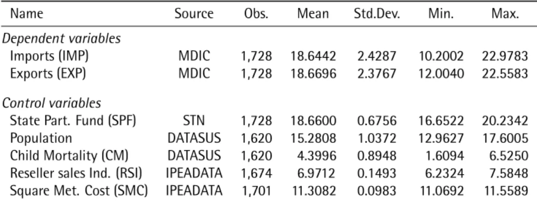
The following variables comprise the�vector: Reseller Sales Index (RSI), Square Meter Cost of construction (SMC), Population, Child Mortality (CM) and States Participation Fund (SPF). Population and Child Mortality (CM) account for the possible role of state size and other idiosyncrasies in affecting its level of imports; Reseller Sales Index (RSI) is a measure of the state economic activity; Square Meter Cost of construction (SMC) accounts for the fact that in states with different costs the share of imports in its expenditures might be different; and States Participation Fund (SPF) is a share of federal taxes which is distributed among states in order to complement their own revenues. Matrix�also contains state, year and month indicator variables, as well as such dummy interactions. Table 5presents the variables sources and their basic statistics.
Table 5presents all the variables in logarithmic form. Therefore 15.2808 represents the logarithm of the population mean5value presented as of 15.2808 and so the population mean is approximately
equal to 7.2 million people and its minimum and maximum values are respectively 426 thousand and 44 million people.
Child Mortality (CM) corresponds to the number of children’s death by state on a monthly basis. CM mean is approximately equal to 121 children’s deaths per month. Reseller Sales Index (RSI) corre-sponds to 100 in the year of 2011, and it is obtained by researching gross sales revenues of reseller firms with more than 20 employees. Finally, Square Meter Cost (SMC) is the price in Brazilian Reais of houses over its area by state on a monthly basis. SMC mean value is equal to R$818.83 and its minimum and maximum values are respectively R$641.65 and R$1,047.04.
Since we are using monthly data and our cross-sectional units are the Brazilian states, the variables available become very limited. Also, the fact that R13 was launched less than three years ago poses additional difficulties. Data on CM and SMC is not available for all states and all periods, so we have an unbalanced panel. This unbalanced panel, however, does not cause any sample selection
Table 5.Variables names, sources and statistics.
Name Source Obs. Mean Std.Dev. Min. Max.
Dependent variables
Imports (IMP) MDIC 1,728 18.6442 2.4287 10.2002 22.9783
Exports (EXP) MDIC 1,728 18.6696 2.3767 12.0040 22.5583
Control variables
State Part. Fund (SPF) STN 1,728 18.6600 0.6756 16.6522 20.2342
Population DATASUS 1,620 15.2808 1.0372 12.9627 17.6005
Child Mortality (CM) DATASUS 1,620 4.3996 0.8948 1.6094 6.5250 Reseller sales Ind. (RSI) IPEADATA 1,674 6.9712 0.1493 6.2324 7.5848 Square Met. Cost (SMC) IPEADATA 1,701 11.3082 0.0983 11.0692 11.5589
Notes:(1) All variables in logarithmic form; (2) MDIC = Ministry of Development, Industry & Foreign Commerce (www .aliceweb.mdic.gov.br); (3) STN = Secretariat of National Treasury (www.tesouro.fazenda.gov.br/pt _PT/transferencias-constitucionais-e-legais); (4) IPEADATA = Institute of Applied Economic Research (www.ipeadata.gov.br); (5) DATASUS = Health Ministry (www2.datasus.gov.br).
issue because in our case the lack of balance is due simply to a limitation on the process of assembling data by the collecting institutions.
5. ESTIMATION RESULTS
5.1. Strategic Interaction Behavior
Table 6presents the results of estimating equation (1) using different weights matrixes. All the variables are in logarithms, except when the random matrix is used. As stated before, the coefficient of interest is the one associated to the spatial explanatory variable�IMP�, defined as the weighted mean of
the importing level of all relevant competing jurisdictions in terms of a particular neighboring rule established by the weighting matrix�.
The coefficient of the spatial explanatory variable�IMP�is negative and statistically significant,
suggesting the existence of strategic interaction among states. The level of imports of a particular state will decrease 0.24 percent if the level of the average imports of its competing states increases one percent. We obtain the largest spatial effect forFWM . The estimated coefficient is approximately -0.49. The high (−0.292) and statistically significant coefficient associated toFWM implies that some relevant part of the states’ strategic interaction is due only to geographical proximity. Indeed, this result is consistent with the fact that FWP tax benefits become less attractive to firms located more distant from the conceding states due to higher logistical and transportation costs.
The coefficient of spatial interaction (�IMP�) in fact is significant at 1% for all four fiscal war
matrixes, except the Random one. Therefore there seems to be evidence of fiscal interaction and that this result is neither a simple consequence of the econometric procedure nor a merely inherent characteristic of underlying data, but it is directly affected by how neighbors are defined, since when we assign weights values randomly we end up with no evidence of strategic interaction.
SPF affects imports negatively and is statistically significant at the 5% level. SPF depends on the states incomeper capita and it is very redistributive. Therefore it is more significant for the poorest states, which, by its turn, present lower levels of imports.
Table 6.Estimation of state interaction on FWP 2010–2015 using different measures of neighbor characteristic.
Explanatory
Variables FWM FWM FWMModel FWM Random
�IMP� −0.2372 −0.4851 −0.4620 −0.2992 0.0068
(0.0842)
***
(0.1061)***
(0.1029)***
(0.0615)***
(0.0207)SPF −0.1398 −0.1403 −0.1396 −0.1228 0.1023
(0.0487)
***
(0.0485)***
(0.0485)***
(0.0485)***
(0.1394)Population −0.9117 −0.8758 −0.8778 −11.116 181.78
(0.4924)
*
(0.4900)*
(0.4900)*
(0.4932)**
(29.723)***
CM −0.0405 −0.0474 −0.0458 −0.0381 −474476
(0.0626) (0.0624) (0.0624) (0.0623) (339047)
RSI 0.3136 0.2954 0.2948 0.3119 −567596
(0.1974) (0.1966) (0.1966) (0.1966) (44219)
SMC 0.0578 0.0387 0.0350 0.0977 7474.1
(0.5280) (0.5245) (0.5247) (0.5238) (2693.7)
***
� 0.17 0.17 0.17 0.17 0.10
Observations 1,620 1,620 1,620 1,620 1620
Notes: (1)FWM= Fiscal War Matrices; (2)FWM , FWM ,FWM andFWM with dependent and explanatory variables in logarithm form; (3) Random Matrix with all variables in level; (4) State, year and month dummy variables omitted; (5) standard error in parenthesis; (6)
*
,**
and***
means significant at 10, 5 and 1% levels respectively; (7)FWM = Matrix with short number of competitor states; (8)FWM = Matrix with large number of competitor states; (9)FWM = Matrix with large number of competitor states excluding SC state; (10)FWM = Matrix with a simple rule of proximity; (11) Random = Matrix with randomly generated weights.level of imports. The negative sign for the Population coefficient is somewhat unexpected since more populous states would presumably present a greater level of imports than the less populated ones. On the other hand a large state also likely produces its own goods, being less dependent on imported goods.
5.2. Impact of R13
Table 7presents the estimation of equation (2), which adds dummy variables to account for a structural change in the strategic interaction among states as a result of the Brazilian Senate Resolution 13 (R13).
As mentioned before, dummy �R13 changes its value from zero to one at the beginning of the
year 2011. However, R13 was put in effect in the beginning of the year 2013, thus if the coefficient of interaction term�R13�IMP
�is statistically significant then there must be some other factors affecting
FWP.
The third column usesFWM and results and a statistically insignificant coefficient of the inter-action term�R13�IMP
�. We also observe these results when we use FWM and FWM in the last
two columns. Only when we useFWM the coefficient is slightly significant.
As we move to the subsequent dummies, all coefficients of interaction become statistically sig-nificant and larger in absolute magnitude.
Table 7. Estimation of R13 effect on FWP 2010–2015 using different FWMs as a measure of neighborhood. Dependent variable:IMP.
Interaction
terms FWM FWM Model FWM FWM
�R13�IMP
� −0.0445 −0.0339 −0.0334 −0.0352
(0.0240)
*
(0.0313) (0.0312) (0.0218)�R13�IMP
� −0.0627 −0.0837 −0.0843 −0.0217
(0.0206)
***
(0.0268)***
(0.0267)***
(0.0180)�R13�IMP
� −0.0700 −0.1078 −0.1093 −0.0090
(0.0218)
***
(0.0282)***
(0.0282)***
(0.0191)�R13�IMP
� −0.0853 −0.1512 −0.1547 −0.0149
(0.0245)
***
(0.0321)***
(0.0323)***
(0.0215)No. of obs. 1,620 1,620 1,620 1,620
Notes: (1)FWM= Fiscal War Matrices; (2) All dependent and explanatory variables in logarithm form; (3)IMP�in the spatial explanatory variable in logarithm of Imports in US dollar FOB; (4) R13are R13
dummy variables; (5) Standard errors in parenthesis; (6)
*
,**
and***
means significant at 10, 5 and 1% levels respectively.January 2014 on, as revealed by the coefficient of the interaction term�R13IMP
�, regardless the weight
matrix.
The exception is when we use FWM and R13 doesn’t affect the strategic interaction among states. Nonetheless, this result is consistent to the notion that fiscal interaction that takes place among states from the same region might have been either less affected or not affected at all by R13, whereas among states that are more distant from each other the strategic interaction is more likely to be affected by R13 as the higher cost of transportation in this case implies less room to profit from the already smaller size of benefits conceded.
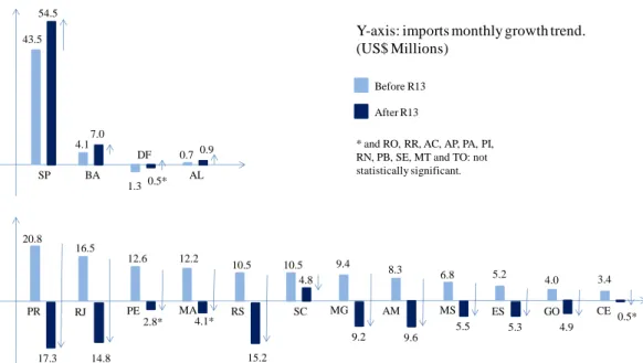
The interaction terms present a negative sign. One can argue that those signs should be positive in order to offset the negative sign of the spatial explanatory variables given inTable 6. Only if this is the case R13 is able to decrease FWP strategic interaction effects. In fact, if R13 has decreased the willingness of states to concede FWP tax benefits, strategic interaction must increase negatively to account for the reverse movement in the imports level growth trend of competing states due to R13, such as shownFigure 1.
Indeed, after R13, the imports growth trend of some states decreased, while the imports growth trend of others states increased even more. Such reverse movement after R13 may be seen as a new movement of interaction among states that is captured in our model as an increase in the absolute value of the strategic interaction. Thus, since the strategic interaction has a negative sign, to increase its absolute value the sign of the terms of interaction between the �R13 dummies and the �IMP
�
spatial variable, such as�R13�IMP
�, must be negative.
One must be careful to analyze Chart 2 once there was an increase in the Dollar/Reais exchange rate6during the period of analysis. However, the increase in the exchange rate was not very important
most of the time (its average value from 2010 to 2012 is 1.8 while its average value from 2013 to 2014 is 2.3).
Figure 1.Growth trend�reversion of some states imports (R13 affected states) against the increase of the growth trend of others states imports (not affected states).
Before R13
After R13
SP 43.5
54.5
Y-axis: imports monthly growth trend. (US$ Millions) 0.9 7.0 BA 20.8 17.3 10.5 4.8 PR SC 10.5 15.2 RS 16.5 14.8 RJ 12.6 2.8* PE 12.2 4.1* MA 9.4 9.2 MG 8.3 9.6 AM 6.8 5.5 MS 5.2 5.3 ES 4.0 4.9 GO 3.4 0.5* CE * and RO, RR, AC, AP, PA, PI,
RN, PB, SE, MT and TO: not statistically significant. AL DF 4.1 0.7 1.30.5*
�Growth trends are the angular coefficient of the adjusted line obtained by OLS regression over importing figures for each state either before or after R13.
Although such reverse movement in imports is probably transitory, and should end in the future when the FWP dynamic reaches a new equilibrium, our model might have been estimated over a period of time not large enough to capture this new equilibrium situation.
The negative sign of the interaction term coefficient could also be a result of the short time horizon of our data compared to the time needed for the economic agents to react to the change in the law.
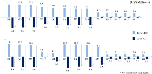
Figure 2presents the growth trend7of the spatial variable�IMP
� both before and after R13,
where� corresponds to theFWM .
Figure 2shows a reversion in the growth trend of the spatial variable�IMP�. In other words, for
each state without exceptions the weighted average value of its competitors’ level of imports presented an increase trend before R13 (before January/2013) and a decrease trend after R13 (since January/2013). As an illustration, the Federal District (DF) spatial variable (�IMP�) was presenting a monthly increase
of approximately US$11.0 million before R13 and a monthly decrease of approximately US$8.9 million after R13.
Therefore, there is some evidence that R13 has changed the spatial interaction among states. Some caution is necessary though because other hidden relevant factors can be affecting imports. Nonetheless, during the period of analysis no other event, other than R13, took place that could explain a change in the states spatial interaction like the one we observed above.
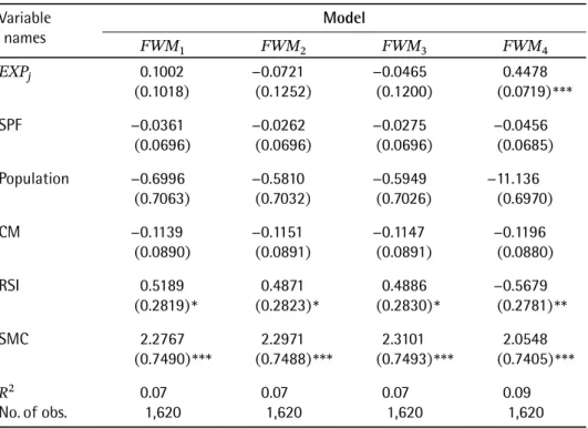
Table 8presents the results of estimating equation (1) using exports instead of imports as the de-pendent variable. The estimation dede-pendent variable (EXP�) and spatial explanatory variable (�EXP�)
both refer to the state’s level of exports, taken in US dollar FOB values.
7Growth trends are the angular coefficient of the adjusted line obtained by OLS regression over�IMP
Figure 2.Growth trend reversion of the spatial variable�IMP�after R13.
Y-axis: W2.IMPj monthly growth trend. (US$ Millions) 11.0 8.9 10.7 8.4 DF SC 10.7 9.8 RS 10.6 8.6 GO 10.4 8.6 MS 3.2 3.6 MT 10.0 8.3 PR 8.2 6.5 AM * TO 2.1 2.0 AC
* Not statistically significant. 11.1 9.1 7.9 6.6 ES CE 7.8 7.0 BA 10.8 8.9 12.6 8.5 8.8 5.6 SP 7.4 6.5 PE 7.4 6.4 MA 3.7 * PB 3.7 * RN 3.6 * PI Before R13 After R13 MG RJ 3.6 * AL 3.6 * SE 3.7 2.1 RR 2.0 2.1 1.9 2.0 2.0 AP PA 1.8 1.9 RO
The idea is to verify if there is no strategic interaction among the states through exports, strength-ening the reliability of the model of strategic interaction over imports.
Second, third, and fourth columns present estimation results using respectivelyFWM ,FWM , and ��� . In all three specifications the spatial explanatory variable is not statistically significant, suggesting no strategic interaction among states with exporting data.
Far from being a proof of inexistence of any type of strategic interaction in the exporting sector, these results only strengthens the reliability of the interaction evidence found in the importing sector. In fact, following a model specification identical to the one used for imports we haven’t found any evidence of strategic interaction using exports figures, which is presumably affected by many factors common to the foreign commerce sector. However, taxation is known to be one major difference8
between the two sides of this sector, the importing and the exporting one. As a result, the strategic interaction found is likely to be due to the taxation factor, in other words, to the possibility of conceding FWP tax benefits in the importing operations.
One single exception is shown in the fifth column ofTable 8, in which we use a fiscal war matrix that forges a simple rule of proximity. Nonetheless, this exception doesn’t constitute a major objection because it could be consequence of one sort of strategic interaction that happens among the same region states due to the high degree of linkage among their economies and that would also affect their exporting activity. For instance, São Paulo (SP) state’s port competes with the Rio de Janeiro (RJ) one, but does not compete with Para (PA) state’s port due to the distance factor.
Thus, the competition in exporting sector between SP and RJ is not driven by the concession of tax benefits because there is no possibility to concede tax benefits in exporting operations, but it is driven simply by their proximity to each other. In other words, since SP and RJ are close to each other, the competition amongst them could still be captured by the model using the proximity matrix.
Table 8.Estimation of state interaction on Exports 2010–2015 using different measures of neighbor characteristic. Dependent variable:EXP.
Variable
names FWM FWM Model FWM FWM
EXP� 0.1002 −0.0721 −0.0465 0.4478
(0.1018) (0.1252) (0.1200) (0.0719)
***
SPF −0.0361 −0.0262 −0.0275 −0.0456
(0.0696) (0.0696) (0.0696) (0.0685)
Population −0.6996 −0.5810 −0.5949 −11.136
(0.7063) (0.7032) (0.7026) (0.6970)
CM −0.1139 −0.1151 −0.1147 −0.1196
(0.0890) (0.0891) (0.0891) (0.0880)
RSI 0.5189 0.4871 0.4886 −0.5679
(0.2819)
*
(0.2823)*
(0.2830)*
(0.2781)**
SMC 2.2767 2.2971 2.3101 2.0548
(0.7490)
***
(0.7488)***
(0.7493)***
(0.7405)***
� 0.07 0.07 0.07 0.09
No. of obs. 1,620 1,620 1,620 1,620
Notes: (1) Using exports figures; (2)FWM = Fiscal War Matrices; (3)FWM , FWM , FWM andFWM
with dependent and explanatory variables in logarithm form; (4) State, year and month dummy variables omitted; (5) standard error in parenthesis; (6)
*
,**
and***
means significant at 10, 5 and 1% levels respectively; (7) FWM = Matrix with short number of competitor states; (8)FWM = Matrix with large number of competitor states; (9)FWM = Matrix with large number of competitor states excluding SC state; (10)FWM = Matrix with a simple rule of proximity.6. CONCLUSION
The purpose of this paper is to evaluate a particular competitive interaction among Brazilian states, the Fiscal War of Ports (FWP). Under the Fiscal War of Ports special tax regimes took the form of tax credits over interstate sales of imported goods. We also evaluate if Resolution 13/2012 (R13), which reduced the tax rate on imported goods in interstate sales, had the desired impact.
Using monthly data on state importing levels in all Brazilian states plus the Federal District during the period from January 2010 to April 2015 we find evidence that Brazilian states do engage in a spatial interaction. The least optimistic estimate indicates that the level of imports of a particular state will decrease by 0.24 percent if the level of imports of its competing states increases by one percent. We also find evidence that R13 has changed the spatial interaction among states since the beginning of 2013 and more deeply in the beginning of 2014.
REFERENCES
Almeida, V. O. (2014). O estado de Goiás na guerra dos portos.Conjuntura Econômica Goiana(28).
Besley, T. J., & Case, A. C. (1995). Incumbent behavior: Vote seeking tax setting and yardstick competition.American Economic Review,85, 25–45.
Brueckner, J. (2000). Welfare reform and the race to the bottom: Theory and evidence. South Economic Journal, 66, 505–525.
Brueckner, J. (2003). Strategic interaction among governments: An overview of empirical studies.International Regional Science Review,26, 175–188.
Brueckner, J., & Saavedra, L. A. (2001). Do local governments engage in strategic property tax competition? National Tax Journey,54, 203–229.
Case, A. C., Rosen, H. S., & Hines, J. C. (1993). Budget spillovers and fiscal policy interdependence: Evidences from the states.Journal of Public Economics,52, 285–307.
Devereux, M. P., Lockwood, B., & Redoano, M. (2007). Horizontal and vertical indirect tax competition: Theory and some evidence from the USA.Journal of Public Economics(91), 451–479.
Dubois, E., & Paty, S. (2010). Yardstick competition: Which neighbours matter?Annals of Regional Science,44(3), 433.
Figlio, D. N., Kolpin, V. W., & Reid, W. (1997). Do states play welfare games? Journal of Urban Economics,46(3), 437–454.
Langemann, E. (2014). A guerra fiscal dos portos e a Resolução 13/12 do Senado Federal: Abrangência, feitos e perspectivas.Indic. Econ. FEE,41(3), 121–132.
Lima, A. C. C., & Lima, J. P. R. (2008). Programas de desenvolvimento local na Região Nordeste do Brasil: Uma avaliação preliminar da guerra fiscal. InXIII Encontro Nacional de Economia Política.
Macedo, F. C. d., & Angelis, A. d. (2013). Guerra fiscal dos portos e desenvolvimento regional no Brasil.Revista de Desenvolvimento Regional,1,(18), 185–212.
Matos, J. G. R., & Das Neves, C. (1999). A guerra fiscal entre os estados brasileiros como arma para atrair os investimentos industriais e as operações de comércio exterior (Unpublished doctoral dissertation). Universidade Federal do Rio de Janeiro, COPPE, Programa de Engenharia de Produção.
Mattos, E., & Politi, R. (2013). Pro-poor tax policy and yardstick competition: A spatial investigation for VAT relief on food in Brazil.Annals of Regional Science,52, 279–307.
Mattos, E., & Rocha, F. (2008). Inequality and size of government: Evidence from Brazilian states. Journal of Economic Studies,35, 333–351.
Mattos, E., Suplicy, M., & Terra, R. (2014). Evidências empíricas de interação espacial das políticas habitacionais para os municípios brasileiros.Economia Aplicada,18, 579–602.
Mello, L. d. (2007, February).The Brazilian “tax war”: The case of value-added tax competition among the states (Working Paper No. 544). OECD Economics Department.
Nascimento, S. P. d. (2008). Guerra fiscal: Uma avaliação comparativa entre alguns estados participantes. Economia Aplicada,12(4).
Novaes, C. S. M. (2014).Possibilidades e limites da arrecadação do ICMS na importação pelo Porto do Itaqui/MA: Elementos conceituais da norma jurídica e de incentivos fiscais(Dissertação de Mestrado). Universidade do Vale do Itajaí, UNIVALI.
Oates, W. E. (2001). Fiscal competition and European Union: Contrasting perspectives. Regional Science and Urban Economics,31, 133–145.
Paiva, D. L., & et al. (2015). A influência do benefício fiscal na escolha do porto marítimo na importação após Resolução 13/2012.South American Development Society JournalSADSJ,1(1), 124–144.
Reich, R. V. M. (2007).Governos benevolentes, governos Leviatã e a (in)eficiência da guerra fiscal(Dissertação de Mestrado, Fundação Getulio Varga, Rio de Janeiro). Retrieved fromhttp://hdl.handle.net/10438/7877 Saavedra, L. A. (2000). A model of welfare competition with evidence from AFDC. Journal of Urban Economics,
47, 248–279.
Shroder, M. (1995). Games the states don’t play: Welfare benefits and the theory of fiscal federalism. Review of Economics and Statistics,77, 183–191.
Silva, C. R. (2012). Guerra fiscal nas importações e a tributação do ICMS: A guerra dos portos(Monografia de Graduação em Direito). Universidade Católica de Brasília.
Silva, L. B., & Almeida, A. F. (2013). Governo federal fixa alíquota de ICMS interestadual em 4% para os produtos importados, independente do estado da federação e tenta acabar com a guerra fiscal entre os portos.Revista de Administração do UNISAL,3(3), 47–62.
Smith, M. W. (1999, August). Should we expect a race to the bottom in welfare benefits? Evidence from a multistate panel, 1979–1995.Retrieved fromhttps://mpra.ub.uni-muenchen.de/10125/
Vieira, D. J. (2014). A guerra fiscal no Brasil: Caracterização e análise das disputas interestaduais por investimentos em período recente a partir das experiências de MG, BA, PR, PE, and RJ. InGovernos estaduais no federalismo brasileiro: Capacidades e limitações governativas em debate(pp. 145–179). Brasilia, DF: IPEA.
APPENDIX.
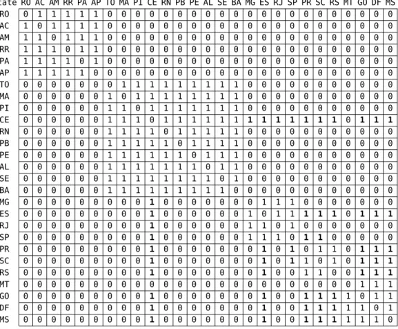
Table A-1presents the first weight matrix, named Fiscal War Matrix nº 1 (FWM ), based on these three criteria. The weight� = is assigned based on the geographical proximity, and activeness in conceding tax breaks, in boldface. In order to make the activeness criteria less arbitrary, we rely on the existent evidence9which indicates that SC, ES, GO, DF, PR, RS, MS, and CE are the most active states on
the Fiscal War of Ports.
A second matrix (FWM ) is assembled exactly the same way as the first one. It includes however 14 states (MG, SP, RJ, ES, PR, SC, RS, AM, BA, MA, PE, CE, GO, MS) plus the Federal District, as the most active in competition. The group of states is enlarged due to new evidence on the FWP.Lima & Lima
(2008), studying a broad set of tax incentive programs issued by Northeast states find out that, in addition to the state of CE, the states of MA, BA and PE are also important players in the foreign commerce fiscal war. For instance, MA has its Industry and Foreign Commerce Tax Incentive Program (SINCOEX), PE has its Pernambuco State Development Program (PRODEPE), and BA has a program of incentives (DESENVOLVE) and an incentive fund (FUNDESE).Vieira(2014) presents a study on the tax incentives conceded by the states of MG, BA, PR, PE, and RJ, showing the various types of incentives they concede, such as deferral of ICMS on import of goods: BA, PE, and RJ; credit grants of ICMS on import of goods: PE; and financing imports: BA and PE.Novaes(2014) studies the state of MA fiscal incentives. Langemann(2014) also mentions the state of AM as a major player due to its special tax zone.
9Prado(1999) points out the existence regional tax incentives regimes in states such as CE since 1966.C. R. Silva(2012) names ES, SC, and GO as important players in the FWP.L. B. Silva & Almeida(2013) analyze SC tax incentive program (PROEMPREGO).
Table A-1.Fiscal War Matrix nº 1 (FWM ).
State RO AC AM RR PA AP TO MA PI CE RN PB PE AL SE BA MG ES RJ SP PR SC RS MT GO DF MS
RO 0 1 1 1 1 1 0 0 0 0 0 0 0 0 0 0 0 0 0 0 0 0 0 0 0 0 0
AC 1 0 1 1 1 1 0 0 0 0 0 0 0 0 0 0 0 0 0 0 0 0 0 0 0 0 0
AM 1 1 0 1 1 1 0 0 0 0 0 0 0 0 0 0 0 0 0 0 0 0 0 0 0 0 0
RR 1 1 1 0 1 1 0 0 0 0 0 0 0 0 0 0 0 0 0 0 0 0 0 0 0 0 0
PA 1 1 1 1 0 1 0 0 0 0 0 0 0 0 0 0 0 0 0 0 0 0 0 0 0 0 0
AP 1 1 1 1 1 0 0 0 0 0 0 0 0 0 0 0 0 0 0 0 0 0 0 0 0 0 0
TO 0 0 0 0 0 0 0 1 1 1 1 1 1 1 1 1 0 0 0 0 0 0 0 0 0 0 0
MA 0 0 0 0 0 0 1 0 1 1 1 1 1 1 1 1 0 0 0 0 0 0 0 0 0 0 0
PI 0 0 0 0 0 0 1 1 0 1 1 1 1 1 1 1 0 0 0 0 0 0 0 0 0 0 0
CE 0 0 0 0 0 0 1 1 1 0 1 1 1 1 1 1 1 1 1 1 1 1 1 0 1 1 1
RN 0 0 0 0 0 0 1 1 1 1 0 1 1 1 1 1 0 0 0 0 0 0 0 0 0 0 0
PB 0 0 0 0 0 0 1 1 1 1 1 0 1 1 1 1 0 0 0 0 0 0 0 0 0 0 0
PE 0 0 0 0 0 0 1 1 1 1 1 1 0 1 1 1 0 0 0 0 0 0 0 0 0 0 0
AL 0 0 0 0 0 0 1 1 1 1 1 1 1 0 1 1 0 0 0 0 0 0 0 0 0 0 0
SE 0 0 0 0 0 0 1 1 1 1 1 1 1 1 0 1 0 0 0 0 0 0 0 0 0 0 0
BA 0 0 0 0 0 0 1 1 1 1 1 1 1 1 1 0 0 0 0 0 0 0 0 0 0 0 0
MG 0 0 0 0 0 0 0 0 0 1 0 0 0 0 0 0 0 1 1 1 0 0 0 0 0 0 0
ES 0 0 0 0 0 0 0 0 0 1 0 0 0 0 0 0 1 0 1 1 1 1 1 0 1 1 1
RJ 0 0 0 0 0 0 0 0 0 1 0 0 0 0 0 0 1 1 0 1 0 0 0 0 0 0 0
SP 0 0 0 0 0 0 0 0 0 1 0 0 0 0 0 0 1 1 1 0 1 1 0 0 0 0 0
PR 0 0 0 0 0 0 0 0 0 1 0 0 0 0 0 0 0 1 0 1 0 1 1 0 1 1 1
SC 0 0 0 0 0 0 0 0 0 1 0 0 0 0 0 0 0 1 0 1 1 0 1 0 1 1 1
RS 0 0 0 0 0 0 0 0 0 1 0 0 0 0 0 0 0 1 0 0 1 1 0 0 1 1 1
MT 0 0 0 0 0 0 0 0 0 0 0 0 0 0 0 0 0 0 0 0 0 0 0 0 1 1 1
GO 0 0 0 0 0 0 0 0 0 1 0 0 0 0 0 0 0 1 0 0 1 1 1 1 0 1 1
DF 0 0 0 0 0 0 0 0 0 1 0 0 0 0 0 0 0 1 0 0 1 1 1 1 1 0 1
MS 0 0 0 0 0 0 0 0 0 1 0 0 0 0 0 0 0 1 0 0 1 1 1 1 1 1 0
A third matrix (FWM ), equal to the second one, except for the fact that it establishes SC as a non-competitor state, is also built. SC can be considered an outlier and as such contaminate the results.