EVIDENCE OF CONSUMERS’ WILLINGNESS TO PAY
FOR THE NATIONAL ANIMAL IDENTIFICATION
SYSTEM OF THE UNITED STATES
Moises A. Resende Filho*
Brian L. Buhr†
Abstract
With the United States National Animal Identification System (NAIS) in place, consumers’ concerns about Bovine Spongiform Encephalopathy (BSE) are mitigated and, by inference, consumers will be willing to pay for the NAIS. We estimated twelve alternative specifications of the gener-alized almost ideal demand system for beef, pork, and poultry, including indexes of news coverage of BSE in the U.S. as proxies for consumers’ risk perception on BSE. Using the preferred model, we constructed scenarios on the basis of hypothesized impacts of the NAIS on consumers’ risk per-ception on BSE in meat. We found that the impact of BSE on consumer de-mand for meat was in itself sufficient to cover previously estimated costs of implementing the NAIS.
Keywords:animal traceability, food safety, system of demand equations, meat industry, USA
JEL classification:C22, Q11, Q13, Q18.
Abstract
Com a implantação do sistema de rastreamento animal (NAIS) dos EUA, as preocupações dos consumidores com respeito ao mal da vaca louca (BSE) serão atenuadas e, por conseguinte, os consumidores estariam dispostos a pagar pelo NAIS. Foram estimadas doze especificações alter-nativas do sistema de equações de demanda generalizado quase ideal para as carnes bovina, suína e de frango, incorporando índices com o número de notícias sobre BSE nos EUA como proxies da percepção de risco dos consumidores. O modelo preferido serviu para construir cenários con-siderando impactos hipotéticos do NAIS sobre a percepção de risco dos consumidores. Conclui-se que o impacto da BSE sobre a demanda por carnes seria suficiente para cobrir estimativas prévias dos custos com a implantação do NAIS.
Keywords: rastreabilidade animal, segurança do alimento, sistemas de equação de demanda, setor de carnes, EUA.
*Departamento de Economia, Universidade de Brasília. E-mail address:[email protected].
†Department of Applied Economics, University of Minnesota. E-mail address:[email protected].
1
Introduction
The United States Department of Agriculture (USDA) Animal and Plant Health Inspection Service (APHIS) had a stated goal of implementing a National Animal Identification System (NAIS) with 100% premises identification and 100% new animal identification by 2009 ( USDA/APHIS 2007a,b). Under this previous Administration, USDA spent more than $120 million, but only 36 percent of producers (500,000 producers) participated (USDA/APHIS 2010).
As a result of concerns about and opposition to NAIS, USDA announced on February 5, 2010, that it will revise the prior animal identification policy and offer a new approach to achieving animal disease traceability (USDA/APHIS
2010). The new framework will only apply to animals moving interstate, but should still allow for finding animal disease, and quickly respond to it. Thus, this new framework is likely to reduce the burden on producers but will not entirely eliminate it.
Although the overall benefit of NAIS is to improve coordination and con-tainment of any disease outbreaks in livestock, it was the discovery of the first U.S. case of Bovine Spongiform Encephalopathy (BSE) or mad-cow dis-ease on December 30, 2003 that accelerated the process for implementation of the NAIS (GRAY, 2004). For instance, the Animal and Plant Health Inspec-tion Service (APHIS) announced, immediately after the first BSE case, a more than tenfold increase in cattle testing relative to previous surveillance levels (Coffey et al. 2005).
Estimated costs of NAIS implementation include increased record keep-ing, animal tagging methods, investments in software and hardware such as scanners if technologies such as radio frequency identification are adopted, increased handling of livestock and other associated costs.
Although producers incur the immediate costs of adopting new technolo-gies, in competitive markets the ability to pass these costs on to consumers depends on the elasticity of demand which depends also on substitution ef-fects. Thus, the question becomes is there evidence that U.S. consumers are willing to pay for the NAIS which would help compensate producers for its implementation? This question is relevant particularly in light of the fact that as shown by Coffey et al. (2005), the primary impact on producers was
gen-erated by a loss of export markets for beef, rather than a decline in U.S. con-sumption. For instance, within days of the discovery of the first case of BSE in a cow in Washington state in 2003, 53 countries, including major markets such as Japan, Mexico, South Korea and Canada, banned imports of U.S. cattle and beef products (Coffey et al. 2005). Meanwhile, these same authors show that
77% of consumers in a regionally targeted survey of U.S. beef consumers did not change their consumption patterns. The banned imports of U.S. cattle and beef products increased domestic supplies and reduced domestic prices, thus negatively impacting producers. However, if U.S. consumers did not reduce their consumption, was the beef price reduction a compensation for them for taking on the increased perceived risk of BSE? If so, this could indicate that NAIS represents a transfer from U.S. consumers and taxpayers to U.S. beef producers and their export market consumers. While beef producers could clearly benefit from increased exports, the focus here is on the impact on do-mestic consumers. As such this paper develops a methodology for assessing whether the U.S. consumer is sufficiently willing to pay for the direct benefits
There are at least two broad approaches to this question. The first is to ask consumers directly as did Hobbs (2003) and Dickinson & Bailey (2002) using market experiments to determine whether consumers were willing to pay for traceability attributes. Criticisms of experimental methods include the issue of the hypothetical nature of experiments, especially in cases where the choice is not imminent (e.g., traceability protecting against a hypothetical contam-ination event). Targeted consumer survey as implemented by Coffey et al.
(2005) is other manner to ask consumers directly. However, while consider-ing the consumption effect, a consumer survey does not address consumers’
willingness to pay.
A second broad approach to analyze consumer willingness to pay is to use an event study that relies on systems of demand equations to assess the im-pact of specific one time and multi-period events on the demand for products. Several studies including Mazzocchi et al. (2004), Burton et al. (1999) and Verbeke & Ward (2001) have employed variations of Almost Ideal Demand Systems (AIDS) for estimating the consumer welfare impacts of issues such as BSE in the U.K. or negative advertising by media regarding meat products. Problems with this approach include: data behavior is often used as a guide to defining the time of impacts which creates endogeneity in the data set; the method can be used to study only a limited number of events over time (lim-ited by identification issues); and this type of modeling does not take into account that modifying the intercept of the AIDS model makes estimates sen-sitive to the units by which quantities and prices are measured.
Recognizing these shortcomings, Alston et al. (2001) show that the use of a Generalized Almost Ideal (GAI) model allows flexible and parsimonious in-corporation of demand shifters in the AIDS model, while obtaining estimates invariant to changes in the units of measurement of quantities and prices. Subsequently, Piggott & Marsh (2004) used the GAI model that incorporates pre-committed quantities and varying intercepts for the expenditure share equations accounting for food safety events’ impact on demand for each meat commodity over time.
Based on the relative merits of those approaches, this paper uses the mod-eling approach firstly taken by Piggott & Marsh (2004) and, subsequently, used by Filho (2008). We expand these previous studies to include BSE as a key food safety issue which has led to the development of NAIS. Although we use the same approach as proposed by Filho (2008) to calculate the con-sumers’ willingness to pay for a risk mitigation strategy such as the NAIS, here we focus only on BSE. Thus, as compared to Filho (2008) this paper adopts a new specification of the news indexes only for BSE, extends the data period through 2006, thereby including actual historical response to the first case of BSE in the U.S. in December 2003, conduct a scenario analysis so to estimate the average value of the NAIS for consumers before and after the first case of BSE in the U.S., and investigate the value of the NAIS under alternative de-grees of consumer’s confidence on the effectiveness of the NAIS. Finally, we
2
Conceptual demand framework
The Generalized Almost Ideal (GAI) model recommended by Alston et al. (2001) is a flexible and parsimonious method of incorporating demand shifters in the Almost Ideal Demand System (AIDS) model and is adapted here for the estimation of willingness to pay for NAIS.
The GAI model originates from a generalized expenditure function given as:
E(p, u) =
N X
i=1
pici+E∗(p, u) (1)
where, pi is the price of goodi,ci is the pre-committed quantity of good i,
p∈RN++is the vector of prices for a group ofNcommodities,PN
i=1pici stands
for the pre-committed expenditure on theN goods, andE∗(p, u) denotes the supernumerary (beyond pre-committed) expenditure. Applying Shephard’s lemma to (1) and using duality identities yields the generalized Marshallian demand function, which when pre-multiplied bypi/xyields the generalized
Marshallian budget share equations as:
wi=pici/x+x∗w∗i(p, x∗)/x ∀i (2)
where,x∗=x−PN
i=1pici is the supernumerary expenditure, andxis the total
expenditure on theNgoods.
The GAI model is obtained by assigning the supernumerary expenditure sharewi∗(p, x∗) to be the AIDS budget share equation given as:
w∗i(p, x∗) =αi+ N X
j=1
γi,jlnpj+βi(lnx∗−lna(p)) ∀i (3)
where lna(p) is the Translog price index given as:
lna(p) =a0+ N X
i=1
αilnpi+
1 2
N X
i=1 N X
j=1
γi,jlnpilnpj (4)
Demand shifters are incorporated in the GAI model to account for time trend, seasonal patterns and food safety indexes for meat (Piggott & Marsh 2004). These demand shifters are introduced in the system of equations by modifying pre-committed quantities, redefiningci’s as:
ci=ci,0+τit+ s−1 X
k=1
θi,kDk+ L X
m=0
φi,mbft−m+πi,mpkt−m+κi,mpyt−m ∀i (5)
wheretis a linear time trend,sdenotes the seasonality, Dkare dummy
vari-ables accounting for seasonal patterns in quarterly meat demand, bft−mare
news events indexes accounting for beef safety issues lagged formquarters,
pkt−m are news events indexes accounting for pork safety issues lagged for
mquarters, andpyt−m are news events indexes accounting for poultry safety
the event remains (length of eventL) also affects demand and is tested within
the model.
Homogeneity of degree zero in prices and expenditure, and symmetry of the Slutsky substitution matrix are imposed on the system’s parameters as maintained hypotheses, as for instance Fisher et al. (2001) and Piggott & Marsh (2004). As the budget shares sum to unity, the error covariance matrix is singular if the system is estimated with all equations included. The equa-tion for poultry is deleted from the system to solve the problem of singularity so that estimates for the parameters of the poultry equation are obtained after system estimation by imposing adding-up constraints.
2.1 Autocorrelation corrections
Under autocorrelation, least square parameter estimates are unbiased and consistent but are not efficient. Moreover, the estimates of the variances of
the estimated parameters are biased and inconsistent (Berndt 1996, p. 477). We use two types of autocorrelation corrections to account for autocorrelation as follows.
Berndt & Savin (1975) showed that maximum likelihood estimation of a system of N−1 equations satisfies invariance, and respects the adding-up constraint if it is imposed that 1′R¯= 0, where1stands for a 1×N vector of ones, and ¯Ris anN×(N−1) matrix with elementsRi,j−Ri,nwherei= 1, . . . , N,
j = 1, . . . , n−1,nindexes the good whose share equation is deleted from the system of equations, andRi,jdenotes the elements of anN×Nautocorrelation
matrixR. Since in practice onlyN−1 equations are estimated, ¯R∗ is a matrix formed by the firstN−1 rows of ¯Rsuch that it is be the firstN−1 elements of ¯R∗ not ¯RorRthat are estimated. This way, the constraint1′R¯ = 0 can be easily imposed after estimating the system of equations (Piggott et al. 1996), even though solving for individual Ri,j is not important (Fisher et al. 2001).
Thus, autocorrelation corrections are incorporated by modifying the original GAI model to:
Wt= ¯R∗Wt−1+ΥtCt−R¯∗Υt−1Ct−1+
x∗t
xt
Wt∗(pt, xt∗)−R¯∗x ∗ t−1
xt−1
Wt∗−1(pt−1, x∗t−1) (6) where
Wt= wwb,t p,t !
,R¯∗= ρb,b ρb,p
ρp,b ρp,p !
,Υt=
pb,t
xt 0
0 pp,t
xt
, Ct=
cb,t
cp,t !
with subscriptsbandpdenoting beef and pork;
Wt∗(pt, xt∗) =
w∗b,t(pt, x∗t)
wp,t∗ (pt, x∗t)
!
;
wi,t are observed shares,pi,t are observed prices at timet; ci,t are
pre-com-mitted quantities as given by (5); and the supernumerary expenditure shares
w∗i,t(pt, xt∗) are AIDS budget equations as given by (3) withx∗treplacingxt.
elements are equal and all offmain diagonal elements are zeros, and a Full
¯
R∗matrix (FRM) wherein its elements are allowed to take in any real value.
3
Data
We use quarterly data from 1982(4) to 2006(4), providing a total of 97 obser-vations, to estimate the system of demand equations. The length of the time series corresponds to Piggott & Marsh (2004) and Filho (2008), but includes updating to 2006 to incorporate post December 2003 when the first BSE case was found in the U.S.
The data series for per capita meat quantities and retail prices are from the US Department of Agriculture, Economic Research Service (USDA/ERS 2006b). USDA calculates quarterly per capita disappearance for meats on a retail weight basis by conversion of the carcass equivalent identity:
per capita disappearance of meat typei= productioni
+ beginning stocksi+ importsi−ending stocksi−exportsi.
Therefore, should an export ban occur (e.g., due to a BSE event) the domestic disappearance will increase one for one by this identity and retail prices will drop to clear the market.
Prices are in dollars per pound for choice retail beef value, pork retail value, chicken as whole fryers retail price and turkey as average U.S. retail prices for whole frozen birds. Following Piggott & Marsh (2004), the time series for poultry quantity is constructed by summing quarterly chicken and turkey quantities in pounds, and poultry prices are quantity weighted sums of chicken and turkey prices.
3.1 BSE news event indexes
According to equation (5), news indexes are incorporated in the system of demand by modifying pre-committed quantities. For purposes of the NAIS we would like to include all animal disease issues, but based on preliminary searches, references to issues such as foot and mouth disease or even avian influenza in the context of poultry were so limited as to be negligible in es-timation of impacts. Therefore, we focused on BSE as a case to calculate the potential value of NAIS related to animal disease outbreaks1.
We used the academic version of Lexis-Nexis news database to compute the number of references to BSE issues found in the top fifty English news-papers in circulation in the US over the entire sample period. A search for BSE news (BSE indexes), which is assumed the reason for putting the NAIS in place, was conducted for the keywords: BSE or Bovine Spongiform
En-cephalopathy or Mad Cow. This search was narrowed to separately collect
beef, pork and poultry information by conducting a search within the pre-viously obtained results with these additional keywords: (a) andbeefor
ham-burger, (b) andporkorham, and (c) andchickenorturkeyorpoultry. Figure 1
shows a plot of the three series of indexes for the period 1982:1 to 2006:4. The large spike in 2003 represents findings of BSE in the U.S. and Canada. Other smaller spikes have occurred on news from placeEurope as well. Ultimately, we obtained series of BSE indexes for beef, pork and poultry as the sum of the number of articles referencing BSE for each quarter.
0 200 400 600 800 1000 1200 1400 1600 1800 2000 19 82 19 83 19 84 19 85 19 86 19 87 19 88 19 89 19 90 19 91 19 92 19 93 19 94 19 95 19 96 19 97 19 98 19 99 20 00 20 01 20 02 20 03 20 04 20 05 20 06 20 07 Year N o . o f R e fe re n ce s beef pork poultry
Figure 1: Beef, pork, and poultry newspaper articles mentioning BSE 1982:1 – 2006:4
One concern of simply using the number of articles to create indexes with no weighting given to content is that any reference is assumed to be inter-preted in the same way by consumers. Clearly, there could be circumstances when beef is portrayed very negatively in the context of a newly found cow with BSE. In another circumstance, an article may describe how the U.S. sur-veillance system is being used to make sure affected cattle will not enter the
human food chain. One would expect this to positively influence consumer preferences for beef. Similarly, U.S. news media could provide stories of BSE found in Japanese cattle which has occurred in recent years. However, cate-gorizing articles over a time series would be highly time intensive and highly subjective to interpretation. Our assumption is that any news of BSE, even good news, raises the prominence of the issue of BSE in the consumer’s mind and is inherently negative.
4
Estimation
The two Full Information Maximum Likelihood (FIML) algorithms to esti-mate the models are the Berndt, Hall, Hall, and Hausman (BHHH) algorithm for maximum likelihood problems and the Marquardt algorithm. These algo-rithms were combined with different starting values for the systems’
Table 1: Tests for the significance of the ‘BSE indexes’ and autocorre-lation corrections
Autocorrelation corrections Lag lengths for BSE indexes H0:NRM H0:DRM H0:NRM H0:No-BSE H0:L= 0 H0:L= 1 Model Ha:DRM Ha:FRM Ha:FRM Model Ha:L= 0 Ha:L= 1 Ha:L= 2 No-BSE 20.308** 5.062 27.540** NRM 18.373** 15.330 19.241** L= 0 20.812** 3.239 23.871** DRM 17.576** 21.246** 10.509 L= 1 25.534** 6.501 31.810** FRM 15.677 24.355** 6.499 L= 2 15.690** 2.597 18.125**
Df 1 3 4 9 9 9
χ20.05,df 3.841 7.815 9.488 16.919 16.919 16.919 Notes: An**denotes the rejection ofH0at the 5% level,Lstands for the lag length of BSE indexes included in models, No-BSE indicates a model estimated with no BSE indexes included,dfdenotes degrees of freedom. Reported test statistics are adjustedLRtests calculated by adjusting the usualLRtest statistic according to equation (7) in the text. Source: Research results.
5
Hypothesis testing and model selection
The adjusted Likelihood Ratio (LR) test was used to test for the most suit-able demand model specification. The reason for this choice is that the usual Likelihood Ratio (LR) is biased toward rejection of restrictions imposed on demand systems in finite samples (Moschini et al. 1994). The adjusted LR test statistic is given by the following formula:
LRs={(M×T−0.5×[(ku+kr)−M×(M+ 1)]M×T}LR (7)
whereLR= 2(LLU−LLR) is the usual likelihood ratio,LLUandLLRare the maximized log-likelihood value in the unrestricted and restricted models;M
is the number of estimated equations;T is the sample size,ku is the number of parameters in the unrestricted model andkr is the number of parameters in the restricted model. The adjustedLRstatistic follows an asymptotic Chi-squared distribution with the number of added variables as degrees of free-dom, under the hypothesis that the additional set of regressors is not jointly significant.
First, we conducted tests for detecting first order autocorrelation in the models estimated with ‘BSE indexes’ as presented in Table 1. For the two classes of models grouped according to the inclusion or not of the BSE in-dexes and to the lag length for inin-dexes (Table 1 from column 2 to column 4), we found that2NRM≻DRM, DRM≻FRM, and FRM≻NRM. These results imply that the final order of preferences for the autocorrelation corrections is DRM≻FRM≻NRM. Therefore, first order autocorrelation in the residu-als is detected in both models, but a ¯R∗ matrix with identical elements in its diagonal is adequate to correct for it.
Second, we investigated the appropriate lag length for BSE indexes within the class of models estimated with a DRM, examining their results reported in the three last columns in Table 1. We observe thatH0: No-BSE is rejected
against Ha: L= 0, H0 :L= 0 is rejected against Ha: L = 1 andH0 :L = 1 is
not rejected against Ha :L = 2. Hence, the order of preferences for models
estimated with a DRMisL= 1≻L= 0≻No-BSE andL= 1≻L= 2. Summing up, for the models estimated with BSE indexes we prefer the one estimated with a DRMand withL= 1 that means consumers have a one quarter memory of BSE news. Filho (2008) found the preferred model did not include any lag length, but he used overall animal diseases news as the basis to construct his indexes, and the period length is also different from the one used here.
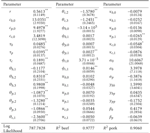
Table 2 presents the estimates for the preferred model. Other complete results are available on request. As shown in Table 2 all intercept estimates of modified pre-committed quantities respectively for beef, pork and poul-try (cb,0,cp,0 andcc,0) are nonnegative, as a priori expected. Except forcc,0,
they are also individually statistically different from zero by the z-test at 5%.
Time trend coefficients (τi,∀i) are all statistically significantly different from
zero, confirming the need for including the time trend variables in the models. With the exception of the coefficient for the first quarter dummy for beefθb,1,
all remaining seasonal coefficients (θi,1, θi,2, θi,3,∀i) are statistically different
from zero by thez-test at 5% of significance across models.
Current own BSE index estimated coefficients for beef (φb,0) and for
poul-try (κc,0) are both negative indicating that BSE references in the news under
the context of beef and poultry respectively depress the pre-committed quan-tities for these two meats. The only own BSE coefficient individually
statisti-cally significant isκc,0.
The only two cross-commodity BSE index coefficients individually
statis-tically different from zero areφp,1 andφc,1. Since both are positive we can
conclude that BSE news in the beef context increases pre-committed quanti-ties for pork and poultry in the quarter following the news report (spillover effect). Except forφp,1 andφc,1, all the other food safety coefficients do not
individually statistically differ from zero by the z-test at 10%. Despite this,
BSE indexes are kept in the model because they are jointly statistically diff
er-ent from zero as found with a series of specification tests used to detect the appropriate lag length for BSE indexes.
6
Expenditure, price and food safety index elasticities
Specific equations and derivations for elasticities in all model forms are avail-able from the authors, but are not provided here because they follow closely the calculations shown in Piggott & Marsh (2004).
Marshallian demand’ elasticities are provided for the direct (on pre-com-mitted quantities demanded) and total (on the total quantities demanded) effects on consumption. Direct elasticities measure the percentage change
in pre-committed quantity of the goodi in response to a 1% increase in the BSE indexes (Piggott & Marsh 2004). BSE index elasticities (Current Direct effect) are given as (8). We do not present the formulas for their lagged version
Table 2: Estimates for the model with a diagonal ¯R∗matrix and with current and one period lagged BSE indexes
Parameter Parameter Parameter
r 0.5613
(0.1149)
** θ
c,2 −1.5780 (0.3678)
** κ
b,0 −0.0079 (0.0124) cb,0 13.0351
(2.9350)
** θc,3 −1.2451 (0.2465)
** κ
b,1 −0.0252 (0.0167) cp,0 9.4978
(1.9277)
** φb,0 −3.14×10⁵
(0.0015) κp,0 −(0.0098)0.0136 cc,0 3.4819
(12.3098) φb,1 (0.0023)0.0017 κp,1 −(0.0129)0.0265 ** τb 0.0485
(0.0276)
* φp,0 0.0007
(0.0015) κc,0 −(0.0304)0.0548 * τp 0.0395
(0.0137)
** φp,1 0.0027 (0.0012)
** κc,1 −0.0876 (0.0538) τc 0.1891
(0.0487)
** φc,0 3.71×10⁻⁵
(0.0044) α0 10(21.0068).6067 θb,1 −0.1177
(0.2104) φc,1 (0.0059)0.0146
** α
b 3.3978 (7.1118) θb,2 0.8310
(0.2331)
** π
b,0 0.0102
(0.0290) αp −(1.1618)0.3876 θb,3 0.9808
(0.1998)
** π
b,1 −0.0048
(0.0327) γbb (3.6041)1.5990 θp,1 −1.0873
(0.1070)
** πp,0 0.0070
(0.0192) γbp (0.6347)0.0435 θp,2 −1.3280
(0.1214)
** π
p,1 −0.0035
(0.0249) γpp −(0.2304)0.1752 θp,3 −1.0866
(0.0930)
** πc,0 0.0544
(0.0666) βb (0.2854)0.4179 θc,1 −2.3600
(0.2706)
** π
c,1 −0.0050
(0.0722) βp −(0.0619)0.0639
Log
Likelihood 787.7828 R
2beef 0.9777 R2pork 0.9060
Notes : numbers in parentheses are the estimated standard errors. An**denotes a coefficient statistically significantly different from zero at the 5% level by thez-test. An*
denotes a coefficient statistically significantly different from zero at the 10% level by the
z-test.cb,0,cp,0andcc,0are intercepts andτb,τp, andτc, are time trend coefficients in the modified pre-committed quantities respectively for beef, pork and poultry.θb,1,θb,2 , and θb,3 are coefficients of the first, second and third seasonal dummies in the modified pre-committed quantity of beef.θp,1,θp,2, andθp,3are coefficients of the first, second and third seasonal dummies in the modified pre-committed quantity of pork.θc,1,θc,2, and θc,3 are coefficients of the first, second and third seasonal dummies in the modified pre-committed quantity of poultry.φb,0,πb,0, andκb,0are the coefficients of beef, pork and poultry BSE indexes with zero lag in the modified pre-committed quantities of beef.φb,1, πb,1, andκb,1are the coefficients of beef, pork and poultry BSE indexes with one lag in the modified pre-committed quantities of beef.φp,0,πp,0, andκp,0are the coefficients of beef, pork and poultry BSE indexes with zero lag in the modified pre-committed quantities of pork.φp,1,πp,1, andκp,1are the coefficients of beef, pork and poultry BSE indexes with one lag in the modified pre-committed quantities of pork.φc,0,πc,0, andκc,0are the
coefficients of beef, pork and poultry BSE indexes with zero lag in the modified
pre-committed quantities of poultry.φc,1,πc,1, andκc,1are the coefficients of beef, pork and poultry BSE indexes with one lag in the modified pre-committed quantities of poultry. α0is the intercept of the Translog price index. ab and ap are the intercepts respectively of the beef and pork share equations.γbb,γbp, andγppare coefficients of the AIDS budget share equations. bb and bp are coefficients of the natural log of the real expenditure with
ωi,bft= φi,0bft
ci,t
∀i
ωi,pkt=
πi,0pkt
ci,t
∀i
ωi,pyt= κi,0pyt
ci,t
∀i
(8)
The a priori expectation is that the own direct demand response to BSE news should be negative for beef. In other words, BSE news related to beef is expected to reduce the pre-committed quantity for this good. It is also expected that the cross effect of BSE news in the beef context will increase the
pre-committed quantities for poultry and pork since substitution is expected to occur in this case. But it is not clear how consumers will react regarding BSE news in the context of poultry and pork (but not with beef mentioned per the search conditions). It may be that news of BSE, even though only affecting beef will cause consumer concern regarding the safety of all meats if
it’s not clear in the article that it only affects beef. On the other hand it may be
expected to increase consumption of pork and poultry as with the cross effect
of BSE news in beef.
Total BSE index elasticities (current total effect) include the sum of the
direct and indirect elasticity given by (9). We do not present the formulas for the lagged BSE index elasticities because it is straightforward to obtain those from the formulas presented in (9).
Ψi,bft =ωi,bft
pi,tci,t
wi,txt
+ 1 + βi
w∗i,t
!bf
t(−pb,tφb,0−pp,tφp,0−pc,tφb,0)
x∗t
wi,t∗ wi,txt
∀i
Ψi,pkt =ωi,pkt
pi,tci,t
wi,txt
+ 1 + βi
w∗i,t
!pk
t(−pb,tπb,0−pp,tπp,0−pc,tπc,0)
x∗t
wi,t∗ wi,txt
∀i
Ψi,pyt =ωi,pyt pi,tci,t
wi,txt
+ 1 + βi
w∗i,t
!py
t(−pb,tκb,0−pp,tκp,0−pc,tκc,0)
x∗t
wi,t∗ wi,txt
∀i
(9)
Our a priori expectation regarding the signals of the total BSE index elas-ticities is that, the final demanded quantities for beef should decrease with more BSE news in the context of beef whereas the demand for pork and poul-try should increase with more BSE news in the context of beef.
The elasticities for the preferred Generalized AIDS model estimated with autocorrelation correction (DRM) and BSE indexes are presented in Table 3.The final elasticities are the sample means of the elasticities computed at every time observation using predicted expenditure shares.
Table 3: Price, expenditure, and food safety elasticities for the generalized AIDS model Estimated with a diag-onal ¯R∗matrix and with current and one period lagged BSE indexes
Marshallian price elasticities
Expenditure elasticities
Hicksian price elasticities
ηb,b −0.502 ηb,x 1.077 ǫb,b −0.148
ηb,p 0.167 ηp,x 0.772 ǫb,p 0.144 ηb,c 0.408 ηc,x 1.018 ǫb,c 0.004
ηp,b 0.179 ǫp,b 0.211 ηp,p −0.507 ǫp,p −0.285 ηp,c 0.086 ǫp,c 0.074
ηc,b 0.563 ǫc,b 0.037
ηc,p 0.265 ǫc,p 0.129 ηc,c −0.190 ǫc,c −0.166
BSE index elasticities Current
direct effect
Lagged direct effect ωb,bf(t) −0.0002 ωb,bf(t−1) 0.0120 ωb,pk(t) 0.0038 ωb,pk(t−1) −0.0019 ωb,py(t) −0.0090 ωb,py(t−1) −0.0299 ωp,bf(t) −0.0074 ωp,bf(t−1) 0.0314 ωp,pk(t) 0.0040 ωp,pk(t−1) −0.0021 ωp,py(t) −0.0237 ωp,py(t−1) −0.0497 ωc,bf(t) 0.0003 ωc,bf(t−1) 0.1098 ωc,pk(t) 0.0228 ωc,pk(t−1) −0.0020 ωc,py(t) −0.0699 ωc,py(t−1) −0.1087
Total current effect
Total lagged effect Ψb,bf(t) −0.0016 Ψb,bf(t−1) −0.0099
Ψb,pk(t) 0.0023 Ψb,pk(t−1) −0.0228
Ψb,py(t) −0.0101 Ψb,py(t−1) −0.0483
Ψp,bf(t) 0.0009 Ψp,bf(t−1) 0.0260
Ψp,pk(t) −0.0019 Ψp,pk(t−1) −0.0002
Ψp,py(t) −0.0247 Ψp,py(t−1) −0.0365
Ψc,bf(t) −0.0281 Ψc,bf(t−1) 0.1138
Ψc,pk(t) 0.0413 Ψc,pk(t−1) 0.0471
Ψc,py(t) −0.0123 Ψc,py(t−1) −0.0146 Notes:ηi,jandǫI,jrepresent the Marshallian and Hicksian price elasticities of demand for theith good with respect to thejth price, andηi,xis expenditure elasticities for theith good, where i, j=bfor beef,pfor pork, andcfor poultry.ωi,kmeasures the percentage change in the pre-committed quantity of theith good in response to a 1% increase in thekth BSE index variable, where k=bf for beef,pkfor pork, andpyfor poultry food safety index, respectively.Ψi,kmeasures the percentage change in the total quantity demanded of theith good in response to a 1% increase in thekth food safety index variable. Estimates shown are the sample means of the elasticities computed at every data point using predicted expenditure shares.
As expected, the own price Hicksian elasticities are all negative. Especially in the case of compensated beef own-price elasticity (−0.148), it indicates that per capita compensated beef consumption changes less, proportionally, than retail price (i.e., beef demand is inelastic) as price changes. The cross-price Hicksian elasticities show that pork, beef and poultry are compensated sub-stitutes one to each other.
The expenditure elasticities indicates that beef and poultry are luxury goods (ηi,x>1 withi =b, c) whereas pork is a necessity (ηp,x<1). Notice that
these elasticities measure how a given meat’s demand changes in response to a change in meat expenditure. Schroeder et al. (2004, p. 11) argues that beef demand expenditure elasticities are generally larger than income elasticities because beef demand is more responsive to changes in meat expenditure than it is to changes in consumer disposable income.
As expected, we observe that for beef the current own BSE index direct elasticity is negative; indicating that BSE news about beef contemporaneously negatively affects its own pre-committed quantities. This is not the case when
we look at the lagged BSE index direct elasticities for beef. It seems that the initial reduction in the pre-committed quantities for beef recovers in the quar-ter afquar-ter a news reference to BSE and beef has occurred.
BSE news under the context of beef will depress as expected the total demand for beef in the current and subsequent period (Ψb,bf(t) =−0.0016, Ψb,bf(t−1)=−0.0099). In addition, BSE news under the context of beef will
increase, in the current and in the next period after their publication, the final demand for pork (Ψp,bf(t)= 0.009, Ψp,bf(t−1)= 0.0260) and for poultry
(Ψp,bf(t)= 0.0281, Ψc,bf(t−1)= 0.1138). Therefore, if the NAIS for beef lower
consumers’ concerns about BSE in beef, this will cause a decrease in pork and poultry demand in current and lagged time.
7
Estimates of the economic value of the NAIS
The simulation of the consumer derived economic value of NAIS is based on the estimates for the preferred model considering a baseline and two scenarios of NAIS as follows.
No NAIS Implementation: The baseline scenario assumes that the NAIS was not implemented in the sample period that makes consumers to change their consumption by the full extent of any media reporting of BSE iden-tified in the search of news articles. This scenario results are obtained by plugging the time series for all exogenous variables into the preferred model to obtain the predicted budget share series for beef, pork and poultry. These series are then multiplied by the total population in the US and the per capita expenditure allocated with meat consumption so to obtain the predicted revenue series that are ultimately converted into real dollar values as of September 2005 using the CPI for all goods.
NAIS Beef: The first scenario assumes that the NAIS was implemented only for beef and dairy cattle through the entire sample period. The only difference from the ‘No NAIS’ baseline scenario, is that the values of the
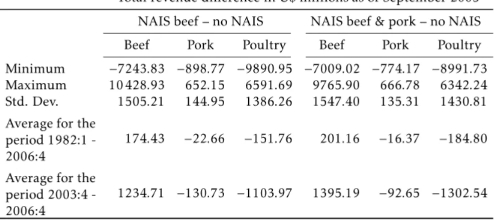
Table 4: Predicted changes in the total revenue for beef, pork and poultry sectors under three alternative scenarios for period 1982:4 - 2006:4 with preferred model of BSE indexes
Total revenue difference in U$ millions as of September 2005 NAIS beef – no NAIS NAIS beef & pork – no NAIS
Beef Pork Poultry Beef Pork Poultry
Minimum −7243.83 −898.77 −9890.95 −7009.02 −774.17 −8991.73 Maximum 10 428.93 652.15 6591.69 9765.90 666.78 6342.24 Std. Dev. 1505.21 144.95 1386.26 1547.40 135.31 1430.81 Average for the
period 1982:1 -2006:4
174.43 −22.66 −151.76 201.16 −16.37 −184.80
Average for the period 2003:4 -2006:4
1234.71 −130.73 −1103.97 1395.19 −92.65 −1302.54
Source: Research results
for identification of animals and elimination of any affected products in
the food chain.
NAIS Beef & Pork: The second scenario assumes that the NAIS was imple-mented for both beef and pork. The only change from the NAIS Beef scenario is that the values of the pork related news indexes are also set to zero.
The average change in quarterly revenue for each meat obtained by com-paring the two scenarios to the baseline are presented in Table 4.
As suggested by the elasticities values, the implementation of the NAIS in-creases the revenue for beef while reducing the revenues of pork and poultry. Over the entire sample period, the implementation of NAIS for beef and pork results in a quarterly gain of $174.433million for the beef industry, but both pork and poultry loss because of the substitution effect with beef so it benefits
the sector with NAIS and the disease concern while taking consumption away from the other. Two factors affect this relationship: (1) the model includes
only meat products and (2) the model has constant expenditures so that gains to one sector must come at the expense of other sectors. As a comparison, preliminary estimates for the costs of the NAIS in the US are $550 million for a five year period (Gray 2004) or an additional cost of $27.5 million per quar-ter for the beef and pork sectors. Another relative benchmark is to consider the total revenue of the beef industry. The total farm value of beef cattle in the U.S. for 2000-2005 averaged approximately $30.2 billion and the average retail value of beef was about $88.8 billion4.
The impact of NAIS is also calculated using the period 2002:4 - 2006:4 only. Clearly, with the U.S. event of BSE, the value of NAIS based on consumer
3Filho (2008) estimated a quarterly gain of $18.34 million for the beef industry which is much lower than $174.43 as we estimated. The main reason for this huge difference is that Resende
Filho (2008) did not consider the period 2003:4 to 2006:4 which is immediately after the discovery of the first case of BSE in the U.S..
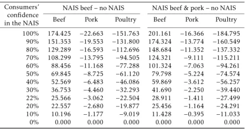
Table 5: Predicted changes in the revenue for beef, pork and poultry sec-tors under three alternative scenarios considering potential reductions in the consumer risk perception about BSE (1982:4−2006:4)
Total revenue difference in million of dollars as of September 2005 Consumers’
confidence in the NAIS
NAIS beef – no NAIS NAIS beef & pork – no NAIS
Beef Pork Poultry Beef Pork Poultry
100% 174.425 −22.663 −151.763 201.161 −16.366 −184.795 90% 151.353 −19.553 −131.800 174.324 −13.774 −160.549 80% 129.289 −16.593 −112.696 148.684 −11.352 −137.332 70% 108.299 −13.795 −94.505 124.321 −9.111 −115.211 60% 88.456 −11.168 −77.288 101.324 −7.063 −94.261 50% 69.845 −8.725 −61.120 79.798 −5.224 −74.574 40% 52.569 −6.483 −46.086 59.869 −3.612 −56.257 30% 36.753 −4.460 −32.293 41.690 −2.250 −39.440 22% 25.566 −3.062 −22.504 28.911 −1.411 −27.499 20% 22.557 −2.680 −19.877 25.456 −1.164 −24.291 10% 10.196 −1.177 −9.019 11.428 −0.395 −11.033
0% 0.000 0.000 0.000 0.000 0.000 0.000
willingness to pay increased dramatically compared to the full sample to a level for beef of $1.234 billion per quarter. Therefore, it is likely that as events such as avian influenza reach the U.S. it will be much more likely to warrant investment in surveillance and recovery systems engendered in systems such as NAIS for poultry as well.
An additional issue is that it is unlikely that NAIS will be 100% effective or
have 100% confidence of consumers – further if there are events which occur that show its ineffectiveness, its credibility will be harmed and subsequent
willingness to pay may be eroded. Therefore, in evaluating NAIS investment it is also important to consider its potential reliability which may be affected
by participation rates as well as information accuracy. To account for this, Table 5 provides a schedule of results pro-rated by the confidence consumers have in the NAIS or in other words, its probability of working. The top row (100%) results are identical to those in Table 4. The results are also inter-preted to show that for the scenario NAIS Beef & Pork, if the NAIS is capable of sustaining the consumers’ confidence at 22% of its level before a BSE news report, the beef sector would afford the additional burden of the NAIS and
consumers would be willing to pay for it. However, the pork sector would never want to see the NAIS implemented because they are harmed with BSE as the primary concern. Similar inferences can be made for other scenarios of implementation, but interesting, fairly low levels would warrant implemen-tation of NAIS.
8
Conclusion
USDA announced on February 5, 2010, that it will revise the prior animal identification policy and offer a new approach to achieving animal disease
(2004) to analyze expected benefits to the meat animal sector from improved confidence consumers may have in the meat supply with an animal identifi-cation system in place. The recent detection of BSE in the U.S. provided the historical news to estimate the impact an event that the NAIS is proposed to help respond. Clearly, there are other potential disease concerns such as foot and mouth disease (FMD) or avian influenza that might also contribute but these are both hypothetical events in the U.S..
A generalized AIDS model was estimated, producing reasonable price elas-ticities for evaluation. However, after correcting for autocorrelation and test-ing for the appropriate lags of the BSE news indexes, only two coefficients
were significantly different from zero, suggesting that it is not clear that the
event of BSE in the U.S. has had a significant impact on consumer demand. This may be due to its relatively recent occurrence as well as its limited scope. This alone suggests that NAIS may be unwarranted, at least in the case of BSE which has been repeatedly described as a remote possibility in U.S. herds.
Never-the-less calculations were completed to estimate the value of the NAIS on meat and poultry markets, and showed that at even relatively low levels estimated in the model, the magnitude can easily exceed cost levels for the implementation of NAIS derived from other sources. Results fur-ther showed that for the estimated coefficients even relatively low adoption of
NAIS or equivalently relatively low reliability (22%) may be enough to war-rant its development.
We recognize shortcomings that deserve further research. First, the model only included meats which preclude the possibility that when an animal dis-ease outbreak occurs consumers would switch to other food products (veg-etables, fruits, etc.). Therefore, our estimates likely under-estimate the value of NAIS in the context of BSE and would surely be greater in the case of a multi-species disease such as foot and mouth disease or avian influenza. Sec-ond, there is significant work that can be done related to parsing out news information and assigning weightings to the content of the information, go-ing beyond simply key-word observations. Despite this, we propose that the methodology used is useful for gaining insight into the prospective benefits, particularly, into how they are distributed among food consumers and pro-ducers.
Bibliography
USDA/APHIS (2007a),Hot Issues: Bovine Spongiform Encephalopathy.
URL:http://www.aphis.usda.gov/lpa/issues/bse/bse-overview.html
USDA/APHIS (2007b),National Animal Identification System (NAIS).
URL:http://animalid.aphis.usda.gov/nais/index.shtml
Alston, J. M., Chalfant, J. A. & Piggott, N. E. (2001), ‘Incorporating demand shifters in the almost ideal demand system’,Economics Letters70, 73 – 78.
Berndt, E. R. (1996),The Practice of Econometrics: Classic and Contemporary, Cambridge: Addison-Wesley Publishing Company.
Berndt, E. R. & Savin, N. E. (1975), ‘Estimation and hypothesis testing in singular equation systems with autoregressive disturbances’, Econometrica
Burton, M., Young, T. & Cromb, R. (1999), ‘Meat consumers’ long-term response to perceived risks associated with bse in great britain’, Cahiers
D’économie et Sociologie Rurales50, 8 – 19.
Coffey, B., Mintert, J., Fox, S., Schroeder, T. & Valentin, L. (2005),The
Im-pact of BSE: A Research Summary, Department of Agricultural Economics
and Kansas State University Agricultural Experiment Station and Cooper-ative Extension Service, Manhattan, USA.
Dickinson, D. L. & Bailey, D. (2002), ‘Meat traceability: Are u.s. consumers willing to pay for it?’,Journal of Agricultural and Resource Economics27, 348 – 364.
Filho, M. A. R. (2008), ‘Potenciais benefícios do sistema de rastreabilidade animal dos eua para o setor de carnes americano’,Revista de Economia e
Soci-ologia Rural46, 1129 – 1154.
Fisher, D., Fleissing, A. R. & Serletis, A. (2001), ‘An empirical comparison of flexible demand system functional forms’,Journal of Applied Econometrics
16, 59 – 80.
Gray, C. W. (2004), The national animal identification system: Basics, blueprint, timelines, and processes,in‘U.S. Livestock Identification Systems: Risk Management and Market Opportunities’, Western Extension Marketing Committee, Tucson, USA.
Hobbs, J. E. (2003), Consumer demand for traceability, Technical report, In-ternational Agricultural Trade Research Consortium.
Mazzocchi, M., Stefani, G. & Henson, S. J. (2004), ‘Consumer welfare and the loss induced by withholding information: The case of bse in italy’,Journal of
Agricultural Economics55, 41 – 58.
Moschini, G., Moro, D. & Green, R. (1994), ‘Maintaining and testing separa-bility in demand system’,American Journal of Agricultural Economics71, 61 – 73.
Piggott, N. E., Chalfant & Alston, J. M. (1996), ‘Demand response to ad-vertising in the australian meat industry’, American Journal of Agricultural
Economics78, 268 – 79.
Piggott, N. E. & Marsh, T. L. (2004), ‘Does food safety information impact u.s. meat demand?’,American Journal of Agricultural Economics86, 154 – 174.
Schroeder, T. C., Marsh, T. L. & Mintert, J. (2004), Beef demand determi-nants, in ‘Report Prepared for the Joint Evaluation Advisory Committee’, Department of Agricultural Economics, Kansas State University, Manhattan, KS, USA.
USDA/APHIS (2010),Questions and Answers: New Animal Disease
Traceabil-ity Framework.
USDA/ERS (2006a),Poultry Yearbook.
URL: http://usda.mannlib.cornell.edu/MannUsda/viewDocumentInfo.do? documentID=1367
USDA/ERS (2006b),Red Meat Yearbook.
URL: http://usda.mannlib.cornell.edu/MannUsda/\viewDocumentInfo.do? documentID=1354
Verbeke, W. & Ward, R. W. (2001), ‘A fresh meat almost ideal demand system incorporating negative tv press and advertising impact’, Agricultural