THE CROSS-CORRELATION BETWEEN OUTPUT
AND NOMINAL VARIABLES IN NEW KEYNESIAN
MODELS CALIBRATED TO BRAZIL AND THE U.S.
Eurilton Araújo*
Abstract
Este artigo investiga se a interação entre formação de hábito e uma regra de Taylor prospectiva consegue reproduzir o padrão de correlação entre produto e variáveis nominais (inflação e taxa de juros) para o Brasil e os Estados Unidos. O estudo emprega um modelo Novo-Keynesiano com rigidez de preço ou de informação. O padrão de correlações vindo dos dados para o Brasil é diferente do padrão para os Estados Unidos. Para ambos os países, os modelos considerados não conseguem reproduzir com um bom grau de precisão os padrões de correlação entre produto e variáveis nominais, embora os modelos de rigidez de preços e de infor-mação impliquem em diferentes mecanismos de propagação dos choques macroeconômicos.
Keywords:correlação cruzada, Novo-Keynesiano, variáveis nominais
Abstract
This paper investigates if the interaction between habit formation and a forward-looking Taylor rule can mimic the observed dynamic correla-tions between output and nominal variables (inflation and interest rates) in Brazil and in the U.S. I carry out the analysis in a new Keynesian model under sticky price or sticky information. The empirical cross-correlation
pattern, obtained from the data, for Brazil is different from the U.S.
pat-tern. For both countries, the models that I considered cannot replicate with a fair amount of accuracy the dynamic correlations between output and nominal variables, though sticky price models and sticky
informa-tion models imply different propagation mechanisms for macroeconomic
shocks.
Keywords:Cross-correlation, new Keynesian, nominal variables
JEL classification:E31, E32, E52
*Banco Central do Brasil and FUCAPE Business School. Email: [email protected]
1
Introduction
In a sequence of papers, Fuhrer & Moore (1995a,b) focused on the ability of alternative specifications of the New-Keynesian Phillips curve to fit inflation persistence and the co-movement between real output and nominal variables. Indeed, Fuhrer & Moore (1995b) present dynamic correlations for the U.S. macroeconomic variables to stress the following robust stylized facts: high levels of inflation anticipate low levels of output and high levels of output anticipate high levels of inflation.
Paez-Farrell (2007, 2008) shows that the new Keynesian model, though ca-pable of replicating impulse response functions from a vector autoregression (VAR) used to identify macroeconomic shocks, cannot easily match the con-temporaneous correlation between output and inflation and the dynamic cor-relations between output and nominal variables (inflation and interest rates) in the U.S. In fact, the new Keynesian model can replicate some characteristics of the co-movement between output and inflation for an implausible param-eterization of the volatility of technology shocks, but at the expenses of the ability to replicate the co-movement between output and interest rates.
Furthermore, María-Dolores & Vázquez (2008) show that the basic new Keynesian model with habit formation as in Fuhrer (2000) can match the co-movement between U.S. output and inflation in the medium-term and long-term horizons, measured by the correlations of VAR forecasting errors of these variables over different forecasting horizons. Den Haan (2000) suggests this
VAR-based methodology to measure the co-movement between economic vari-ables by means of dynamic contemporaneous correlations. For each horizon considered, the information set is different, providing a rich picture of how
contemporaneous correlations may evolve over time. Thus, this measure can be more informative about the dynamic interaction between economic vari-ables than unconditional correlations.
In a recent paper, Cassou & Vázquez (2010) extend the methodology of Den Haan (2000) to compute correlations between output and inflation at dif-ferent horizons, and propose a model to explain the observed patterns. The model features a very high degree of habit persistence, which generates a rich looking structure in demand, introducing additional forward-looking terms in the traditional IS curve. To a certain extent, this model is capable of replicating the dynamic correlation patterns at different horizons
as long as the right balance between the effects of supply and demand shocks
obtains through a calibration method that resemble the simulated method of moments.
In this paper, I ask whether variants of the model investigated in María-Dolores & Vázquez (2008) can replicate the dynamic correlations between output and nominal variables in Brazil and in the U.S. I carry out the analysis in a new Keynesian model under sticky price or sticky information since the correlation patterns may depend on the interaction between habit persistence and the nature of the price-setting behavior. Therefore, this study extends the work of Paez-Farrell (2008), by focusing on the role of the following features: habit formation, a forward-looking Taylor rule and alternative price-setting schemes. These elements were absent in the variants of the new Keynesian model he investigated.
cross-correlation between output and the interest rate.
Compared with María-Dolores & Vázquez (2008) and Cassou & Vázquez (2010), which considered habit formation and hybrid Phillips curves, I inves-tigate the role of a forward-looking Taylor rule as well as the effect of
sticky-information as introduced by Mankiw & Reis (2002). In addition, this paper studies two different economies: Brazil, an emerging economy, and the U.S.
In short, this paper therefore differs from previous papers by
consider-ing alternative theories for inflation dynamics, by incorporatconsider-ing a forward-looking Taylor rule with an explicit role for inflation expectations in monetary policy and by explicitly analyzing two distinct economies, Brazil and the U.S. I summarize the main findings in this paragraph. First, Brazil and the U.S. display somewhat different cross-correlation patterns between output and
nominal variables (inflation and the interest rate). Second, the models con-sidered cannot match, with a fair amount of accuracy, the cross-correlation pattern in the data for Brazil and for the U.S. For Brazil, due to the high degree of uncertainty implied by simulated confidence bands, the empirical correlations are within these bands, though the simulated mean cross-correlations are far from the observed cross-cross-correlations. For the U.S., the models do not improve much upon the traditional new Keynesian specifica-tion. In fact, introducing habit formation and a forward-looking Taylor rule did not help much, especially in capturing the dynamic relationship between inflation and the output gap. Further, dynamic responses of output, inflation and the interest rate are somewhat different for the sticky price compared to
the sticky information specification, especially the response to supply shocks. This feature may explain the different shapes for the mean simulated
cross-correlations across alternative price-setting specifications.
This paper proceeds as follows. The second section presents observed dy-namic correlations between output and nominal variables for Brazil and the U.S. under alternative filtering techniques used to remove the output trend. The third section introduces the variant of the new Keynesian model sug-gested by María-Dolores & Vázquez (2008) under alternative price-setting schemes. The fourth section presents the results concerning the role of habit formation and forward-looking Taylor rules in replicating the dynamic corre-lations between output and nominal variables in models with sticky prices or sticky information. The fifth section discusses impulse response analysis of key macroeconomic variables to demand and supply shocks under the two alternative price-setting shemes. Finally, the sixth section concludes.
2
Measuring the dynamic correlations between output and
nominal variables
2.1 Brazil
For Brazil, the data come from the IFS database of the IMF. I use quarterly observations on real GDP, consumer price inflation and T-Bill rates, starting at the first quarter of 1995 and ending in the last quarter of 2010. I report the asymptotic two standard error bounds. Since the sample is very short, only 64 observations, just few dynamic correlations, concerning output and lagged interest rate are different from zero. In fact, the bounds are a decreasing
func-tion of the sample size and their magnitudes in absolute values are relatively large compared with the observed dynamic correlations. The motivation for choosing such small sample is the necessity to exclude the Brazilian hyperin-flationary period with several structural breaks and unstable macroeconomic environment. I therefore focus on a period of stable inflation.
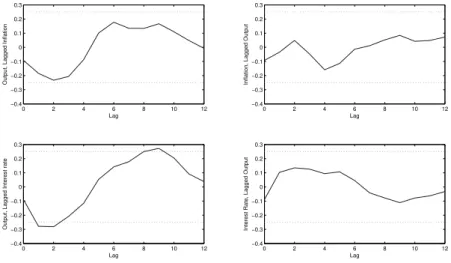
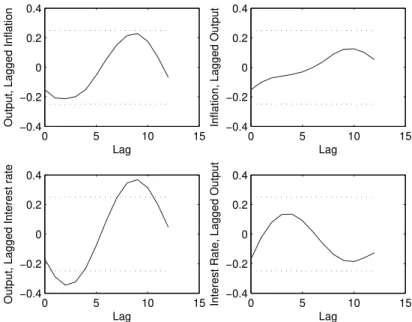
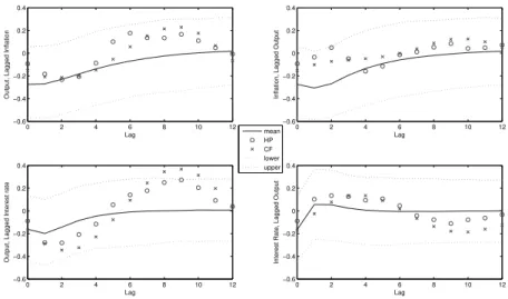
Inspecting figures 1 and 2, no statistically significant pattern emerges. Considering the correlations between lagged inflation and the output gap, as well as the correlations between lagged interest rates and the output gap, they are negative for short lags and a positive pattern emerges for long lags. The correlation pattern concerning inflation and the lagged output gap, though not so clear depending on the filtering techniques, tend to be negative for short lags. Using the Christiano-Fitzgerald filter, the dynamic correlations are negative for short lags and positive for long lags, increasing monotonically. Fi-nally, the dynamic correlations between interest rates and the lagged output gap have negative values for short lags, positive magnitudes for intermediate lags and negative values for long lags.
The contemporaneous correlation between the output gap and inflation and the contemporaneous correlation between the output gap and the interest rate are both negative.
0 2 4 6 8 10 12
−0.4 −0.3 −0.2 −0.1 0 0.1 0.2 0.3
Lag
Output, Lagged Inflation
0 2 4 6 8 10 12
−0.4 −0.3 −0.2 −0.1 0 0.1 0.2 0.3
Lag
Inflation, Lagged Output
0 2 4 6 8 10 12
−0.4 −0.3 −0.2 −0.1 0 0.1 0.2 0.3
Lag
Output, Lagged Interest rate
0 2 4 6 8 10 12
−0.4 −0.3 −0.2 −0.1 0 0.1 0.2 0.3
Lag
Interest Rate, Lagged Output
0 5 10 15 −0.4
−0.2 0 0.2 0.4
Lag
Output, Lagged Inflation
0 5 10 15
−0.4 −0.2 0 0.2 0.4
Lag
Inflation, Lagged Output
0 5 10 15
−0.4 −0.2 0 0.2 0.4
Lag
Output, Lagged Interest rate −0.40 5 10 15 −0.2
0 0.2 0.4
Lag
Interest Rate, Lagged Output
Figure 2: Cross Correlations – CF Band Pass Filter - Brazil
2.2 U.S.
I use the same quarterly sample as Cassou & Vázquez (2010), starting in the first quarter of 1965 and ending in the last quarter of 2008. The data comes from the FRED database of the Federal Reserve Bank of Saint Louis. The mea-sure of inflation is the log difference in GDP deflator and the interest rate is
the Fed Funds rate. I use the output gap measure based on real GDP data as computed by the Bureau of Economic Analysis. In all figures, since the sample is relatively large, I report the approximate asymptotic two standard error bounds to identify in which lags the dynamic correlations are statisti-cally different from zero, taking therefore into account the uncertainty in the
estimated correlations.
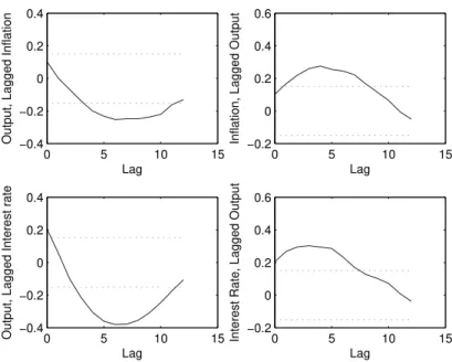
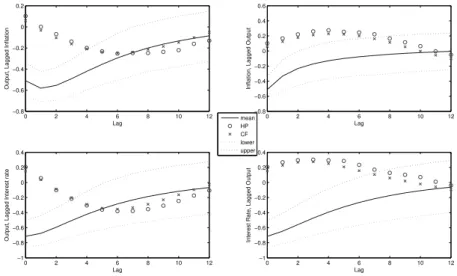
For the U.S., the dynamic correlations between the output gap and infla-tion show that high inflainfla-tion anticipates lower levels of output gap from three to eleven quarters later. Further, high interest rates also anticipate lower out-put gaps. These effects are statistically significant. In addition, the output
gap positively leads inflation from one to eight quarters. This is also true for the interest rates. Again, these positive dynamic correlations are statistically significant. These results are consistent with the empirical evidence reported in Fuhrer & Moore (1995b) and in Cassou & Vázquez (2010), and the dynamic correlations concerning the output gap and inflation are in line with the find-ings in Wang & Wen (2007). Moreover, they are robust to alternative filtering techniques.
0 5 10 15 −0.4
−0.2 0 0.2 0.4
Lag
Output, Lagged Inflation
0 5 10 15
−0.2 0 0.2 0.4 0.6
Lag
Inflation, Lagged Output
0 5 10 15
−0.4 −0.2 0 0.2 0.4
Lag
Output, Lagged Interest rate −0.20 5 10 15 0
0.2 0.4 0.6
Lag
Interest Rate, Lagged Output
Figure 3: Cross Correlations – HP Filter - U.S.
0 5 10 15
−0.4 −0.2 0 0.2 0.4
Lag
Output, Lagged Inflation
0 5 10 15
−0.2 0 0.2 0.4 0.6
Lag
Inflation, Lagged Output
0 5 10 15
−0.4 −0.2 0 0.2 0.4
Lag
Output, Lagged Interest rate −0.20 5 10 15 0
0.2 0.4 0.6
Lag
Interest Rate, Lagged Output
2.3 Discussion
The dynamic correlation patterns for Brazil are different from the U.S. Diff
er-ences in the degree of economic development, institutional arrangements and country’s history might explain the diversity in the dynamic correlations be-havior reported in 2.1 and 2.2. Another important feature probably driving the results is the very short sample considered in the case of Brazil, covering quarterly data from the period of stable inflation.
Moreover, there isn’t a priori reasoning justifying the absence of country-dependence in establishing a set of stylized facts concerning cross-correlations. Dynamic correlation patterns tend to be heterogeneous even if the countries studied are more homogeneous. Indeed, for 18 OECD countries, the cross-correlations between the output gap and inflation reported in Wang & Wen (2007) support this claim.
In the following sections, I will ask if variants of the new Keynesian model can match at least qualitatively the patterns described in 2.1 and 2.2.
2.4 The Models
In this section, I briefly describe the artificial economies studied. Since the specifications feature standard building blocks which previous research used extensively, I describe the structure of the model with more details in the ap-pendix. Rather than describe each economic agent and its constraints in this section, I provide references that discuss the specifics of the new Keynesian framework I use in this paper, referring the reader to the appendix for further details.
Galí (2008) presents the basic new Keynesian model in chapter 3. The ex-tended version with habit formation follows the discussion in Dennins (2009). To be more specific, I use the multiplicative habit specification described in
Fuhrer (2000). The period utility function isu(Ct) =11
−1τ
Ct Ctγ−1
1−1τ
. Dennins (2009) compares alternative strategies to modeling habit formation and con-cludes that up to a first order approximation, business cycle properties are independent of the chosen approach to modeling habit formation. Dennins (2009), however, does not address the issue concerning the role of habit for-mation for the co-movement between real and nominal variables.
Galí & Gertler (1999) discussed extensively the hybrid version of the new Keynesian Phillips Curve. I use the version based on dynamic indexation pro-posed by Smets & Wouters (2003), which Dennins (2009) uses to complete the supply-side of the models he discussed.
The following expressions describe the log-linear approximations of the first order conditions characterizing the equilibrium in the extended version of the new Keynesian model with habit persistence and a hybrid new Keyne-sian Phillips curve.
τ+1+1βγ−βγ2+γ(1−τ)
yt=γ1(1−βγ−τ)yt−1+
h
τ+1+βγ1−(1+βγγ)(1−τ) i
Etyt+1
+βγ(1−τ)
1−βγ Etyt+2−τ(it−Etπt+1) +gt (1)
πt=
β
1 +ωβEtπt+1+ κ
1 +ωβyt+ ω
I use the following notation:yt,πt,andit denote the output gap and the
deviations from the steady states of inflation and interest rates, respectively. The condconclusiitional expectation operator based on the information set available to agents at time t isEt. In addition, gt andzt stand for aggregate
demand and supply shocks. These shocks follow first-order auto-regressive processes:
gt=ρggt−1+εgt zt=ρzzt−1+εzt
The shocks εgt and εzt are normally distributed random variables with
mean zero and variancesσg2andσz2, respectively.
Equation 1 is the log-linear approximation of the consumption Euler equa-tion with the specificaequa-tion of habit formaequa-tion described in Fuhrer (2000). The parameter β is the inter-temporal discount factor of the representative con-sumer. The pconclusiarameter τ is the inverse of the relative risk aversion parameter in a constant relative risk aversion utility function. Finally, the parameterγ measures the degree of habit persistence. The absence of habit formation is the situation in whichγ= 0 and, consequently, the inertial term in the Euler equation vanishes.
Equation 2 is a hybrid new Keynesian Phillips curve in whichωis the frac-tion of firms in the Calvo (1983) set up that can revise their prices according to lagged inflation, though unable to re-optimize them. The absence of iner-tia in inflation is the situation in whichω= 0, and equation 2 becomes the canonical new Keynesian Phillips curve.
The following Taylor-type rules describe monetary policy.
it=ρit−1+ (1−ρ)(ψ1πt+ψ2yt) +vt (3)
it=ρit−1+ (1−ρ)(ψ1Etπt+1+ψ2Etyt+1) +vt (4)
Equation 3 is an interest rate rule in which the central bank responds con-temporaneously toπtandyt. Equation 4 is an interest rate rule in which the
central bank responds to forecasts of inflation and the output gap, denoted byEtπt+1 andEtyt+1. In both specifications, the parameterρcaptures
inter-est rate persistence. The coefficients of the Taylor rule areψ1 andψ2, andvt
denotes a normally distributed monetary policy shock with varianceσv2.
The contemporaneous Taylor rule, described in equation 3, was used in Paez-Farrell (2007, 2008), María-Dolores & Vázquez (2008) and Cassou & Vázquez (2010). To isolate the effects of habit persistence under alternative
In addition to the new Keynesian Phillips curve described in equation 2, based on a sticky price model of price-setting behavior, I consider a version of the Phillips curve based on Mankiw & Reis (2002). The basic idea is that information disseminates slowly in the economy. In each period, a fractionλ
of firms obtains new information on the state of the economy and computes
optimal prices based on this information. The fraction 1−λ of firms
con-tinues to set prices based on outdated information. The assumption about information arrival is analogous to the assumption about price-stickiness in the traditional sticky-price model of Calvo (1983). The following expression describes the sticky-information Phillips curve.
πt=
λα
1−λ
yt+λ
∞
X
j=0
(1−λ)jEt−1−j[πt+α(yt−yt−1)] +zt (5)
The parameterαconnects real marginal costs to the output gap, and usu-ally depends on the specification of the utility function in the case of constant returns to scale technology using only labor as input. Under sticky informa-tion, I drop equation 2 from the system and, instead, use 5 as a description of the supply side of the model.
The results in Paez-Farrell (2007, 2008), as well as in María-Dolores & Vázquez (2008), emphasize that the structure of the canonical new Keynesian model leads to more important effects of aggregate supply shocks relative to
aggregate demand shocks. One way to generate co-movement is to specify an empirically implausible ratio between the variances of these shocks. An alternative strategy is to alter some structural features of the canonical model to induce larger effects of aggregate demand shocks vis-à-vis aggregate
sup-ply shocks. The introduction of habit formation and a forward-looking Tay-lor rule increases the relative importance of aggregate demand shocks, allow-ing more forward-lookallow-ing agents to react instantly to demand related shocks. Larger effects of aggregate demand shocks will also depend on which type of
rigidity is driving inflation dynamics in a particular model. Therefore, it is important to consider alternative inflation dynamics theories (sticky prices or sticky information).111
3
Results
3.1 Calibration
I consider the specifications described in table 1 and table 2. Table 1 concerns the sticky-price version of the model. The first specification, in this table, denoted by Model 1, is the canonical new Keynesian model, without habit formation (γ=0), without a backward-looking component in inflation (ω=0) and with a contemporaneous Taylor rule featuring interest rate smoothing as
in equation 3. Model 2 has no habit formation (γ=0), a hybrid new
Table 2 shows the specifications I consider under sticky-information. The first specification, in this table, denoted by Model 5, has no habit formation (γ=0), and a contemporaneous Taylor rule featuring interest rate smoothing as in equation 3. Model 6 has an Euler equation with habit formation and a contemporaneous Taylor rule featuring interest rate smoothing as in equation 3. Model 7 has the same structural characteristics as Model 6, but monetary policy follows a forecast-based Taylor rule featuring interest rate smoothing as in equation 4. Table 3 summarizes the parameterization I use for the different
specifications of the model.
Brazil
To calibrate the new Keynesian model, I take parameter values forβ,ωand
κfrom Silveira (2008), who estimated a DSGE model using Brazilian data. I also use his estimation for the Taylor rule parameters. The high value forγ, around 0.6, reported in Silveira (2008) induced indeterminacy. Therefore, I calibrate this parameter with the same magnitude used in the US case. These values are consistent with estimated values reported in McDermott & Mc-Menamin (2008) for a semi-structural new Keynesian model fitted to Latin American countries in the post inflation-target regime. The parameters for the sticky information Phillips Curve come from Caetano & Moura (2009). These parameters are actually the mean values for the estimated parameters that they report under different settings. The shocks’ calibration follows Bugarin
& Freitas (2007).
The U.S.
Following María-Dolores & Vázquez (2008), I calibrate the parameters ac-cording to the estimates in Lubik & Schorfheide (2004). The U.S. calibration follows tables 1 and 3 in María-Dolores & Vázquez (2008). The degree of habit persistence is slightly different from 0.25, reported in María-Dolores &
Vázquez (2008). For the sticky information model, I follow the calibration in Mankiw & Reis (2002) concerning the parameters governing inflation dynam-ics.
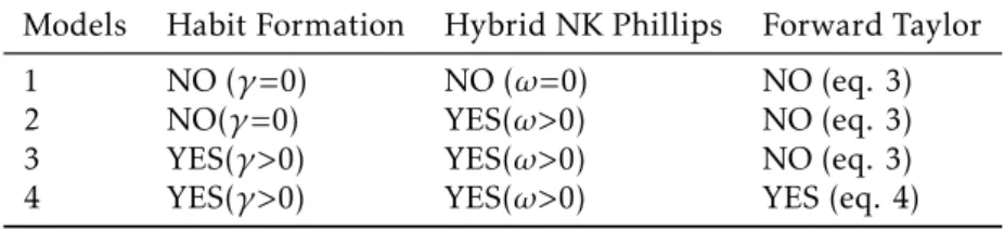
Table 1: Specifications for the Sticky-Price Model
Models Habit Formation Hybrid NK Phillips Forward Taylor
1 NO (γ=0) NO (ω=0) NO (eq. 3)
2 NO(γ=0) YES(ω>0) NO (eq. 3) 3 YES(γ>0) YES(ω>0) NO (eq. 3) 4 YES(γ>0) YES(ω>0) YES (eq. 4)
3.2 Findings
Table 2: Specifications for the Sticky-Information Model
Models Habit Formation Forward Taylor
5 NO (γ=0) NO (eq. 3)
6 YES(γ>0) NO (eq. 3) 7 YES(γ>0) YES (eq. 4)
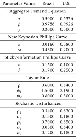
Table 3: Calibration
Parameter Values Brazil U.S.
Aggregate Demand Equation
τ 0.5000 0.5376
β 0.9758 0.9926
γ 0.3000 0.3000
New Keynesian Phillips Curve
κ 0.0160 0.5800
ω 0.4500 0.2000
Sticky-Information Phillips Curve
α 0.1500 0.1000
λ 0.1700 0.2500
Taylor Rule
ρ 0.6000 0.8400
ψ1 1.5000 2.1900 ψ2 0.8000 0.3000
Stochastic Disturbances
ρg 0.3400 0.8300
σg 0.1500 0.1800
ρz 0.7000 0.8500
σz 0.0300 0.6400
values for dynamic correlations compatible with the ones based on a finite sample. Therefore, for each specification described in tables 1 and 2, I will assess if the observed dynamic correlations are within the confidence bands generated by the model.
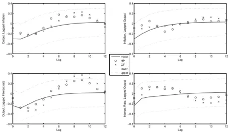
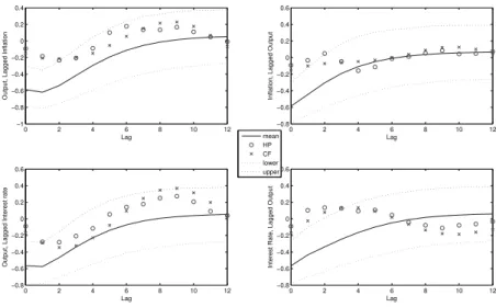
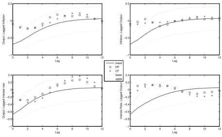
Figures 5 to 18 present the dynamic correlations between output and two nominal variables (inflation and interest rates) for Brazil (figures 5 to 11) and for the U.S. (figures 12 to 18). The figures report lower and upper bounds based on 95% confidence intervals (dotted lines). For each specification, I obtain these bounds from simulated time series. The circled line denotes ob-served dynamic correlations in which I use the Hodrick-Prescott (HP) filter to compute the output gap. The x-marked lined denotes observed dynamic cor-relations in which I use the Christiano and Fitzgerald filter (CF) to compute the output gap. The solid line represents the average dynamic correlations across simulations.
Brazil
Figures 5 to 11 show the results for Brazil. The first remark is that the confi-dence bands generated by simulation are very large. Therefore, in a statistical sense, the models are capable of generating the cross-correlation pattern ob-served at least for lags greater than 3.
In the standard new Keynesian model, this is the case even for short lags. The introduction of a hybrid Phillips curve or habit persistence, in the new Keynesian specifications, makes the upper bound for the correlations very negative for short lags. This is not consistent with the small negative magni-tudes of the cross-correlations for short lags. Interestingly, the new Keynesian models capture very well the cross-correlations between inflation and lagged output for lags greater than 4. In addition, the magnitudes of the correlations between output and lagged inflation, as well as the correlations between out-put and lagged interest rates, tend to be higher in the data compared to the mean across simulations, especially for long lags.
0 2 4 6 8 10 12
−0.6 −0.4 −0.2 0 0.2 0.4
Lag
Output, Lagged Inflation
0 2 4 6 8 10 12
−0.6 −0.4 −0.2 0 0.2 0.4
Lag
Inflation, Lagged Output
0 2 4 6 8 10 12
−0.6 −0.4 −0.2 0 0.2 0.4
Lag
Output, Lagged Interest rate
0 2 4 6 8 10 12
−0.6 −0.4 −0.2 0 0.2 0.4
Lag
Interest Rate, Lagged Output
mean HP CF lower upper
0 2 4 6 8 10 12 −1 −0.8 −0.6 −0.4 −0.2 0 0.2 0.4 Lag
Output, Lagged Inflation
0 2 4 6 8 10 12
−0.8 −0.6 −0.4 −0.2 0 0.2 0.4 0.6 Lag
Inflation, Lagged Output
0 2 4 6 8 10 12
−0.8 −0.6 −0.4 −0.2 0 0.2 0.4 0.6 Lag
Output, Lagged Interest rate
0 2 4 6 8 10 12
−0.8 −0.6 −0.4 −0.2 0 0.2 0.4 0.6 Lag
Interest Rate, Lagged Output
mean HP CF lower upper
Figure 6: Brazil Model 2 (sticky price, no habit, hybrid and no forward)
0 2 4 6 8 10 12
−1 −0.5 0 0.5
Lag
Output, Lagged Inflation
0 2 4 6 8 10 12
−1 −0.5 0 0.5
Lag
Inflation, Lagged Output
0 2 4 6 8 10 12
−1 −0.8 −0.6 −0.4 −0.2 0 0.2 0.4 Lag
Output, Lagged Interest rate
0 2 4 6 8 10 12
−1 −0.8 −0.6 −0.4 −0.2 0 0.2 0.4 Lag
Interest Rate, Lagged Output
mean HP CF lower upper
0 2 4 6 8 10 12 −1 −0.5 0 0.5 Lag
Output, Lagged Inflation
0 2 4 6 8 10 12
−1 −0.5 0 0.5
Lag
Inflation, Lagged Output
0 2 4 6 8 10 12
−1 −0.8 −0.6 −0.4 −0.2 0 0.2 0.4 Lag
Output, Lagged Interest rate
0 2 4 6 8 10 12
−1 −0.8 −0.6 −0.4 −0.2 0 0.2 0.4 Lag
Interest Rate, Lagged Output
mean HP CF lower upper
Figure 8: Brazil Model 4 (sticky price, habit, hybrid and forward)
For almost all lags, the sticky information models, irrespective of exhibit-ing habit persistence or a forward-lookexhibit-ing Taylor rule, are consistent with the observed cross-correlations. In fact, the upper bounds are positive or mildly negative. In spite of that fact, the empirical correlations tend to be more dis-perse relatively to mean of the simulations. In fact, the mean of the simulated correlations between output and lagged inflation, as well as the correlations between output and lagged interest rates, are flatter in the sticky information specifications compared to the sticky price models, especially for long lags.
0 2 4 6 8 10 12
−0.5 −0.4 −0.3 −0.2 −0.1 0 0.1 0.2 0.3 Lag
Output, Lagged Inflation
0 2 4 6 8 10 12
−0.5 −0.4 −0.3 −0.2 −0.1 0 0.1 0.2 0.3 Lag
Inflation, Lagged Output
0 2 4 6 8 10 12
−0.6 −0.4 −0.2 0 0.2 0.4 Lag
Output, Lagged Interest rate
0 2 4 6 8 10 12
−0.4 −0.3 −0.2 −0.1 0 0.1 0.2 0.3 0.4 Lag
Interest Rate, Lagged Output
mean HP CF lower upper
0 2 4 6 8 10 12 −0.6
−0.4 −0.2 0 0.2 0.4
Lag
Output, Lagged Inflation
0 2 4 6 8 10 12
−0.6 −0.4 −0.2 0 0.2 0.4
Lag
Inflation, Lagged Output
0 2 4 6 8 10 12
−0.6 −0.4 −0.2 0 0.2 0.4
Lag
Output, Lagged Interest rate
0 2 4 6 8 10 12
−0.6 −0.4 −0.2 0 0.2 0.4
Lag
Interest Rate, Lagged Output
mean HP CF lower upper
Figure 10: Brazil Model 6 (sticky information, habit and no forward)
0 2 4 6 8 10 12
−0.6 −0.4 −0.2 0 0.2 0.4
Lag
Output, Lagged Inflation
0 2 4 6 8 10 12
−0.6 −0.4 −0.2 0 0.2 0.4
Lag
Inflation, Lagged Output
0 2 4 6 8 10 12
−0.8 −0.6 −0.4 −0.2 0 0.2 0.4 0.6
Lag
Output, Lagged Interest rate
0 2 4 6 8 10 12
−0.8 −0.6 −0.4 −0.2 0 0.2 0.4 0.6
Lag
Interest Rate, Lagged Output
mean HP CF lower upper
U.S.
Figures 12 to 18 show the results associated with the U.S. economy. Figures 12 to 15 report the dynamic correlations for the sticky price models. Model 1 predicts a very strong negative co-movement in all lags. Therefore, the canon-ical new Keynesian specification cannot account for the dynamic correlations between output and nominal variables. Paez-Farrell (2008) documents very well this inability of the canonical new Keynesian model.
The introduction of backward-looking terms, first in the Phillips Curve and next in the dynamic Euler equation (the IS curve), does not change that characteristic very much. The forward-looking Taylor rule does not help ei-ther. The models, however, are able to match the dynamic correlation pat-terns for long lags, since they are negative. In fact, for the correlation between the output gap and lagged nominal variables, the observed values are within the bands for lags approximately greater than four. The observed correlations between nominal variables and the lagged output gap lie inside the bands for lags approximately greater than seven. On the other hand, the positive values for the correlations associated with short lags are difficult to match.
0 2 4 6 8 10 12
−0.8 −0.6 −0.4 −0.2 0 0.2
Lag
Output, Lagged Inflation
0 2 4 6 8 10 12
−0.8 −0.6 −0.4 −0.2 0 0.2 0.4 0.6
Lag
Inflation, Lagged Output
0 2 4 6 8 10 12
−1 −0.8 −0.6 −0.4 −0.2 0 0.2 0.4
Lag
Output, Lagged Interest rate
0 2 4 6 8 10 12
−1 −0.8 −0.6 −0.4 −0.2 0 0.2 0.4
Lag
Interest Rate, Lagged Output
mean HP CF lower upper
Figure 12: U.S. Model 1 (sticky price, no habit, no hybrid and no forward)
0 2 4 6 8 10 12 −0.8 −0.6 −0.4 −0.2 0 0.2 Lag
Output, Lagged Inflation
0 2 4 6 8 10 12
−0.8 −0.6 −0.4 −0.2 0 0.2 0.4 0.6 Lag
Inflation, Lagged Output
0 2 4 6 8 10 12
−1 −0.8 −0.6 −0.4 −0.2 0 0.2 0.4 Lag
Output, Lagged Interest rate
0 2 4 6 8 10 12
−1 −0.8 −0.6 −0.4 −0.2 0 0.2 0.4 Lag
Interest Rate, Lagged Output
mean HP CF lower upper
Figure 13: U.S. Model 2 (sticky price, no habit, hybrid and no forward)
0 2 4 6 8 10 12
−0.8 −0.6 −0.4 −0.2 0 0.2 Lag
Output, Lagged Inflation
0 2 4 6 8 10 12
−0.8 −0.6 −0.4 −0.2 0 0.2 0.4 0.6 Lag
Inflation, Lagged Output
0 2 4 6 8 10 12
−1 −0.8 −0.6 −0.4 −0.2 0 0.2 0.4 Lag
Output, Lagged Interest rate
0 2 4 6 8 10 12
−1 −0.8 −0.6 −0.4 −0.2 0 0.2 0.4 Lag
Interest Rate, Lagged Output
mean HP CF lower upper
0 2 4 6 8 10 12 −0.8 −0.6 −0.4 −0.2 0 0.2 Lag
Output, Lagged Inflation
0 2 4 6 8 10 12
−0.6 −0.4 −0.2 0 0.2 0.4 Lag
Inflation, Lagged Output
0 2 4 6 8 10 12
−1 −0.8 −0.6 −0.4 −0.2 0 0.2 0.4 Lag
Output, Lagged Interest rate
0 2 4 6 8 10 12
−1 −0.8 −0.6 −0.4 −0.2 0 0.2 0.4 Lag
Interest Rate, Lagged Output
mean HP CF lower upper
Figure 15: U.S. Model 4 (sticky price, habit, hybrid and forward)
hand, the models in figures 16 to 18 do not capture the correlations between lagged output and inflation. Finally, results in figure 17 do not change when I use a forward-looking Taylor rule in the simulations (figure 18).
0 2 4 6 8 10 12
−1 −0.8 −0.6 −0.4 −0.2 0 0.2 0.4 Lag
Output, Lagged Inflation
0 2 4 6 8 10 12
−1 −0.8 −0.6 −0.4 −0.2 0 0.2 0.4 Lag
Inflation, Lagged Output
0 2 4 6 8 10 12
−1 −0.8 −0.6 −0.4 −0.2 0 0.2 0.4 Lag
Output, Lagged Interest rate
0 2 4 6 8 10 12
−1 −0.8 −0.6 −0.4 −0.2 0 0.2 0.4 Lag
Interest Rate, Lagged Output
mean HP CF lower upper
Figure 16: U.S. Model 5 (sticky information, no habit and no forward)
0 2 4 6 8 10 12 −0.8 −0.6 −0.4 −0.2 0 0.2 0.4 0.6 Lag
Output, Lagged Inflation
0 2 4 6 8 10 12
−1 −0.8 −0.6 −0.4 −0.2 0 0.2 0.4 Lag
Inflation, Lagged Output
0 2 4 6 8 10 12
−0.4 −0.2 0 0.2 0.4 0.6 0.8 1 Lag
Output, Lagged Interest rate
0 2 4 6 8 10 12
−0.2 0 0.2 0.4 0.6 0.8 1 1.2 Lag
Interest Rate, Lagged Output
mean HP CF lower upper
Figure 17: U.S. Model 6 (sticky information, habit and no forward)
0 2 4 6 8 10 12
−0.6 −0.4 −0.2 0 0.2 0.4 Lag
Output, Lagged Inflation
0 2 4 6 8 10 12
−1 −0.8 −0.6 −0.4 −0.2 0 0.2 0.4 Lag
Inflation, Lagged Output
0 2 4 6 8 10 12
−0.4 −0.2 0 0.2 0.4 0.6 0.8 1 Lag
Output, Lagged Interest rate
0 2 4 6 8 10 12
−0.2 0 0.2 0.4 0.6 0.8 1 1.2 Lag
Interest Rate, Lagged Output
mean HP CF lower upper
4
The Propagation of Shocks
According to Cassou & Vázquez (2010), impulse responses of key macroeco-nomic variables to demand (εgt) and supply (εzt) shocks can trace to some
extent the pattern of lead and lag correlations. The difficult step in
repro-ducing the cross-correlations pattern is to achieve the right balance between these shocks. In general, a variable X will lead a variable Y if the impact of a particular shock on X dies out more quickly compared to the impact on Y. In contrast to Cassou & Vázquez (2010), I do not calibrate the model to get the right correlation pattern. My goal is to assess the differences in
im-pulse response functions between the sticky price and the sticky information models. I use the U.S. calibration and the model with all features that I am investigating with potential to enhance the ability of the models to induce a cross-correlation pattern more in line with the data. Thus, I am considering model 4 in table 1 and model 7 in table 2 as the specifications for impulse response analysis.
Figures 19 to 22 show impulse responses to demand and supply shocks to the models. The variables y, infla and r denote output, inflation and the interest rate, respectively. According to figure 19, in the sticky price model, output leads the interest rate after a demand shock, but output and inflation seem to have approximately the same degree of persistence, therefore there is no tendency of lelag relationship between output and inflation. In ad-dition, these variables move in the same directions after the shock. Figure 20 show the responses after a supply shock. All variables respond in a very persistent way, indicating that there is no tendency of lead-lag relationship between these variables. After the supply shock, output moves in the oppo-site direction compared to inflation and the interest rate, which increase after the supply shock.
2 4 6 8 10 12 14 16 18 20
−1 0 1
y
2 4 6 8 10 12 14 16 18 20
−1 0 1
infla
2 4 6 8 10 12 14 16 18 20
0 0.1 0.2
r
2 4 6 8 10 12 14 16 18 20 −2
−1 0
y
2 4 6 8 10 12 14 16 18 20
0 0.2 0.4
infla
2 4 6 8 10 12 14 16 18 20
0 0.05 0.1
r
Figure 20: Impulse Response to supply shocks –sticky price model
Concerning the sticky information model, figure 21 shows that inflation tends to lead both output and the interest rate after a demand shock, since in-flation is less persistent. Output and the interest rate display more or less the same degree of persistence. Again, all variables move in the same direction as in the sticky price model. Figure 22 shows impulse responses to the sticky information model after a supply shock. All variables respond in a very per-sistent way and the contraction in output is much stronger compared to the sticky price model, leading to a decrease in interest rates.
Though the qualitative pattern of response after a demand shock is similar across models, the comparative degree of persistence is not. In contrast to the sticky price model, the sticky information model delivers a different response
pattern after a supply shock. This diversity in responses after demand and supply shocks, combined with different sizes for the variances of the shocks,
explain the different shapes in cross-correlation functions from the alternative
models discussed in 4.2.
5
Conclusions
This paper extends the work in María-Dolores & Vázquez (2008) and Paez-Farrell (2008), and investigates if an extended version of the new Keynesian model featuring habit formation, forward-looking Taylor rules and alternative price schemes can mimic the dynamic correlations between output and two nominal variables (inflation and interest rates) in Brazil and in the U.S.
The models considered cannot offer a significant improvement in
2 4 6 8 10 12 14 16 18 20 −1
0 1
y
2 4 6 8 10 12 14 16 18 20
−1 0 1
infla
2 4 6 8 10 12 14 16 18 20
0 0.1 0.2
r
Figure 21: Impulse Response to demand shocks –sticky information model
2 4 6 8 10 12 14 16 18 20
−2 −1 0
y
2 4 6 8 10 12 14 16 18 20
0 0.2 0.4
infla
2 4 6 8 10 12 14 16 18 20
0 0.05 0.1
r
data, the extended models cannot reproduce the fact that inflation systemati-cally lags output.
Compared with Cassou & Vázquez (2010), I did not attempt to calibrate the models in order to match the lead and lag patterns concerning the dy-namic correlation between output and nominal variables. Instead, I evaluated how alternative features not considered in Cassou & Vázquez (2010) may im-prove the performance of macroeconomic models in replicating the dynamic cross-correlations between output and nominal variables. To this end, I used calibrations based on previously estimated parameters.
According to Cassou & Vázquez (2010), the models need to get the right relative proportions for the supply and demand shock variances, as well as the relative persistence of these shocks. Since the results reported did not endorse a great improvement relatively to the basic new Keynesian model, in light of the findings in Cassou & Vázquez (2010), supply and demand shocks were not in the right proportion in order to match the lead and lag patterns in the data for both countries.
Though Cassou & Vázquez (2010) calibrated their model in order to match the dynamic correlation patterns, the parameter values they reported may be at odds with the data in other dimensions and may not be the most likely parameterization in a full-information context. Just to be more specific, the method these authors used was a limited-information approach, close to the simulated methods of moments, and there are multiple parameters configu-rations compatible with the lead and lag patterns in the data, therefore such calibration was not unique. Thus, it is prudent to regard the parameteriza-tions reported by these authors with some degree of skepticism.
In short, in contrast to Cassou & Vázquez (2010), I did not search for the parameters that would reproduce the patterns shown in the data. Instead, I used parameters from previous estimations, usually based on full information likelihood methods. In addition, I explored alternative features that could improve the basic new Keynesian model. The results show that these fea-tures alone under plausible calibrations are not enough to match the cross-correlation patterns shown in the data with a good degree of accuracy. Thus, this paper corroborates Cassou & Vázquez (2010), showing that a delicate com-bination between supply and demand shocks rather than the introduction of more structural or semi-structural features are extremely important in repli-cating the dynamic correlations between output and nominal variables.
This inability to reproduce important characteristics of the output-inflation dynamics seems to be a drawback of other models incorporating nominal, real or informational rigidities. Wang & Wen (2007) show that alternative new Keynesian models, featuring sticky information or price stickiness, can-not match important characteristics of the output-inflation dynamics. The investigation of the joint implications of different forms of real and nominal
rigidities for the co-movement between real and nominal variables seems to be a fruitful area for future research.
6
Acknowledgements
and suggestions. The views expressed in this paper are my own and do not necessarily reflect those of the Banco Central do Brasil
Bibliography
Bugarin, M. & Freitas, P. (2007), ‘A study on administered prices and optimal monetary policy’, SBE, XXIX Encontro Brasileiro de Econometria.
Caetano, S. & Moura, G. (2009), ‘Reajuste informacional no brasil: uma apli-cação da curva de phillips sob rigidez de informação’, ANPEC, XXXVII En-contro Nacional de Economia .
Calvo, G. (1983), ‘Staggered prices in a utility-maximizing framework’, Jour-nal of Monrtary Economics12, 383–398.
Cassou, S. & Vázquez, J. (2010), ‘New keynesian model features that can reproduce lead, lag and persistence patterns.’.
Christiano, L., Eichenbaum, M. & Evans, C. (2005), ‘Nominal rigidities and the dynamic effects of a shock to monetary policy,’,Journal of Political
Econ-omy113, 1–45.
Christiano, L. J. & Fitzgerald, T. J. (2003), ‘The band pass filter’,International Economic Review44, 435–465.
Coibion, O. (2010), ‘Testing the sticky information phillips curve’,The Re-view of Economics and Statistics,92, 87–101.
Den Haan, W. J. (2000), ‘The co-movement between output and prices’, Jour-nal of Monetary Economics46, 3–30.
Dennins, R. (2009), ‘Consumption habits in a new keynesian business cycle model’,Journal of Money41, 1015–1030.
Fuhrer, J. (2000), ‘Habit formation and its implications for monetary policy
models’,American Economic Review90, 367–390.
Fuhrer, J. C. & Moore, G. R. (1995a), ‘Inflation persistence’,Quarterly Journal of Economics110(1), 127–159.
Fuhrer, J. C. & Moore, G. R. (1995b), ‘Monetary policy trade-offs and the
correlation between nominal interest rates and real output’, The American Economic Review85(1), 219–239.
Galí, J. (2008),Monetary Policy, Inflation, and the Business Cycle. An Introduc-tion to the New Keynesian Framework.
Galí, J. & Gertler, M. (1999), ‘Inflation dynamics: A structural econometric analysis’,Journal of Monetary Economics44, 195–222.
Kydland, F. & Prescott, E. (1990),Business Cycles: Real Facts and a Monetary Myth, Federal Reserve Bank of Minneapolis.
Lubik, T. & Schorfheide, F. (2004), ‘Testing for indeterminacy: an application to us monetary policy,’,American Economic Review94, 190–217.
Mankiw, N. G. & Reis, R. (2002), ‘Sticky information versus sticky prices: A proposal to replace the new keynesian phillips curve,’,The Quarterly Journal of Economics,117, 1295–1328.
María-Dolores, R. & Vázquez, J. (2008), ‘The new keynesian monetary model: Does it show the comovement between gdp and inflation in the us?’,Journal of Economic Dynamics32, 1466–1488.
McDermott, J. & McMenamin, P. (2008), ‘Assessing inflation targeting in latin america with a dsge model’, Central Bank of Chile Working Paper.
Paez-Farrell, J. (2007), ‘Output and inflation in models of the business cycle with nominal rigidities: further counterfactual implications’,Scottish Journal of Political Economy54, 475–491.
Paez-Farrell, J. (2008), ‘Assessing sticky price models using the burns and mitchell approach’,Applied Economics40, 1387–1397.
Silveira, M. (2008), ‘Using a bayesian approach to estimate and compare new keynesian dsge models for the brazilian economy: the role for endogenous persistence.’,Revista Brasileira de Economia,62, 333–357.
Smets, F. & Wouters, R. (2003), ‘An estimated stochastic dynamic general equilibrium model of the euro area’,Journal of the European Economic Associ-ation1, 1123–1175.
Wang, P. & Wen, Y. (2007), ‘Inflation dynamics: A cross-country investiga-tion’,Journal of Monetary Economics54, 2004–2031.
Appendix A
The Models
A.1 Sticky-Price Model
The Representative Consumer
The lifetime utility is:U =E0P∞t=0βt
1 1−1τ
Ct Ctγ−1
1−1τ
−υN
1−ϕ t
1+ϕ
The variable Ct stands for aggregate consumption, Nt is the amount of
labor offered by the representative consumer in the job market. The parameter τis the relative risk aversion of the agent. The parameterγcontrols the degree
of habit persistence in consumption. In addition, the parameters υ and ϕ
control labor supply. The parameterβ, between zero and one, is the inter-temporal discount factor.
The representative consumer maximizes U, subject to the following budget constraint:
The variableBtstands for the nominal bond. The lettersWt andPtrepresent
nominal wages and prices. The letterit is the nominal interest rate on bonds.
The consumer maximizes U subject to the budget constraint.
The Representative Firm
There is a continuum of firms, indexed by j, which operate a linear technology, according to the linear production functionYt(j) =AtNt(j), in whichAtstands
for an aggregate technology shock. They produce differentiated goods, which
compose a final aggregate consumption good, represented by
Yt= Z 1
0 Y
ε−1
ε t (j)dj
!ε−ε1
,
whereεis the elasticity of substitution.
The environment is that of monopolistic competition, therefore the firm can choose its price. Following the Calvo (1983) scheme of pricing, a particu-lar firm may reset its price with a probability given by 1−θin any given time, independently of the time elapsed since the last price was set. Therefore, a fraction 1−θ of the firms set prices, while another fraction ofθ keep their previous prices, without any change.
Firms maximize the discounted profits, taking into account that they will not be able to change the prices, unless they receive a green light to do so with probability1−θ.
Following Christiano et al. (2005), I introduce an indexation mechanism in which firms that do not set prices optimally at time t will adjust their prices to lagged inflation, according to the equationPt+i =Pt+i−1(j) (πt+i−1)
ω, where
the parameterωindicates the degree of price indexation. The variablesPtand
πtdenotes the price level and inflation.
The optimal price set by firms allowed to change prices isP∗
t and the
ag-gregate price level evolves according to the expression:
Pt= h
θ(Pt−1(πt−1)
ω)1−ε+ (1
−θ) (Pt∗)1−ε i11
−ε
The derivation of the supply side of the model is standard and advanced macroeconomics textbook describe it in details. For instance, Galí (2008) de-velops the algebra step-by-step. In the neighborhood of zero steady state in-flation, the New Keynesian Phillips Curve characterizes inflation dynamics according to equation 2. The expression for the parameterκisκ=(1−βθ)(1−θ)
θ .
The parameterκis strictly decreasing inθ, a measure of the degree of nominal price rigidity.
Monetary Policy is described by Taylor rules in equations 3 and 4
A.2 Sticky-Information Model
The Representative Consumer
The Representative Firm
I follow the description presented in Mankiw & Reis (2002) Every firm sets prices every period t, but the information needed to update prices optimally flows slowly over time. In each period, a fractionλof the firms obtains new information about the economy, which they use to compute the updated path for optimal prices. The remaining firms set prices based on outdated informa-tion. The arrival of information is such that each firm has the same probability of being one of the firms that gather new information, regardless of how long it has been since its last informational update. In this context, the optimal price isp∗
t=pt+αyt. The variablesptandytare the price level and the output
gap in logarithmic scale.
A firm that last updated its information set j periods ago sets price accord-ing to the followaccord-ing expression: xtj=Et−j(pt∗). The aggregate price level is the average of prices of all firms deciding prices at the period t, which is:
pt=λ
∞
X
j=0
(1−λ)jxjt=λ
∞
X
j=0
(1−λ)jEt−j(pt+αyt) (I)
By taking out the first term and redefining the index in the sum, this equa-tion becomes:
pt=λ(pt+αyt) +λ
∞
X
j=0
(1−λ)j+1Et−1−j(pt+αyt) (II)
The previous period price is:
pt−1=λ ∞
X
j=0
(1−λ)jEt−1−j(pt−1+αyt−1) (III)
Subtracting (III) from (II), inflationπtevolves according to the equation:
πt=λ(pt+αyt) +λ
∞
X
j=0
(1−λ)j+1Et−1−j[πt+α(yt−yt−1)]
+λ2 ∞
X
j=0
(1−λ)jEt−1−j(pt+αyt) (IV)
By rearranging equation (II), I can show that
pt−
αλ
1−λ
yt=λ
∞
X
j=0
(1−λ)jEt−1−j(pt+αyt) (V)
I use equation (V) to substitute for the last term in equation (IV). After some algebra, the final expression is:
πt=
λα
1−λ
yt+λ
∞
X
j=0
(1−λ)jEt−1−j[πt+α(yt−yt−1)]
The final expression is equation 5 in section 3 of the paper, without the exogenous cost-push shock.
Appendix B
Filtering Techniques and Simulations
This appendix provides some references on the filtering methods used to com-pute the output gap and details on how I conducted simulations on the models I considered in this paper.
B.1 Filtering Techniques
To compute the output gap, I use two different filters. The first one is the
tra-ditional Hodrick-Prescott Filter, discussed in Kydland & Prescott (1990), with smoothing parameters equals to 1600 (the standard specification for quarterly data). The second method I used to extract the output cyclical component is a band pass filter proposed by Christiano & Fitzgerald (2003). This filter ex-tracts the components related to the business cycles (frequencies associated with eight to thirty two quarters), eliminating very low and very high fre-quency movements in the data.
B.2 Simulations