ABSTRACT: Reference Governor is an important component of Active Fault Tolerant Control. One of the main reasons for using Reference Governor is to adjust/modify the reference trajectories to maintain the stability of the post-fault system, especially when a series of actuator faults occur and the faulty system can not retain the pre-fault performance. Fault estimation error and delay are important properties of Fault Detection and Diagnosis and have destructive effects on the performance of the Active Fault Tolerant Control. It is shown that, if the fault estimation provided by the Fault Detection and Diagnosis (initial “fault estimation”) is assumed to be precise (an ideal assumption), the controller may not show an acceptable performance. Then, it is shown that, if the worst “fault estimation” is considered, it will be possible to reduce the effects of fault estimation error and delay and to preserve the performance of the controller. To reduce the effects of this conservative assumption (worst “fault estimation”), a quadratic cost function is deined and optimized. One of the advantages of this method is that it gives the designer an option to select a less sophisticated Fault Detection and Diagnosis for the mission. The angular velocity stabilization of a spacecraft subjected to multiple actuator faults is considered as a case study.
KeywoRdS: Active Fault Tolerant Control, Fault estimation error and delay, Reference Governor, Angular velocity stabilization.
Reducing the Effects of Inaccurate Fault
Estimation in Spacecraft Stabilization
Rouzbeh Moradi1, Alireza Alikhani1, Mohsen Fathi Jegarkandi2
INTRODUCTION
Active Fault Tolerant Control (AFTC) is an important ield in automatic control that has attracted a large amount of attention. he main responsibility of an AFTC is to tolerate component malfunctions while maintaining desirable performance and stability properties of the faulty system (Zhang and Jiang 2008). Latterly, a review paper published recent developments of the spacecrat AFTC system (Yin et al. 2016).
One of the main components of any AFTC is the Fault Detection and Diagnosis (FDD) module. here are several challenges that FDD designs have in common (Zhang and Jiang 2008). Among them, fault estimation error and delay are considered in this paper. hese challenges have destructive efects on the stability and performance (Zhang and Jiang 2008). Reference Governor (RG) is one of the components of the general AFTC structure (Zhang and Jiang 2008). The terms Command Governor (CG) and Reference Trajectory Management (RTM) have been also used in the literature. he main responsibility of RG is to adjust/modify the reference trajectories, so the post-fault model of the system remains stable, even ater the occurrence of multiple actuator faults (Garone et al. 2016). here are several papers in the literature that have studied the efects of RG on the performance and stability of the post-fault model (Boussaid et al. 2010; Boussaid et al. 2011; Boussaid et al. 2014; Almeida 2011). According to these papers, RG has been able to deal with the actuator faults/ failures eiciently.
To the authors’ best knowledge, reducing the efects of fault estimation error and delay using the concept of RG still remains an open problem. This is the main subject that is pursued in this paper. It is shown that, as long as the estimated fault
1.Ministry of Science, Research and Technology – Aerospace Research Institute – Astronautics Department – Tehran/Tehran – Iran. 2.Sharif University of Technology – Engineering College – Department of Aerospace Engineering – Tehran/Tehran – Iran.
Author for correspondence: Alireza Alikhani | Ministry of Science, Research and Technology – Aerospace Research Institute – Astronautics Department | PO box: 14665-834 – Tehran/Tehran – Iran | Email: [email protected]
reported by the FDD (initial “fault estimation”) is assumed to be precise (an ideal assumption), the controller may not show an acceptable performance.
However, if the maximum fault estimation error is considered (worst “fault estimation”), RG can be used to reduce the ef ects of FDD errors and preserve the performance of the closed-loop system. To reduce the ef ects of this conservative assumption (considering maximum fault estimation error), a quadratic cost function is dei ned and optimized.
In order to validate the results, the angular velocity stabilization of a spacecrat subjected to multiple actuator faults is considered. It is shown that, if the initial “fault estimation” (the fault estimation reported by the FDD) is considered accurate, the response will not converge to the origin. However, if RG is designed based on the worst “fault estimation”, AFTC will be able to asymptotically stabilize the faulty spacecrat in a wide range of actuator fault and despite FDD errors. h is paper consists of the following sections: i rstly, the modeling of the proposed RG is described. h en, the spacecrat dynamics and controller are shown. Finally, results obtained and the discussions are presented.
MODELING THE REFERENCE GOVERNOR
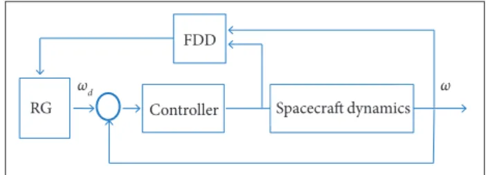
h e structure of the considered AFTC is shown in Fig. 1. It is assumed that the FDD block provides “an estimation of ” the post-fault model of the system. h e RG block uses the proposed methodology to i nd the most suitable reference trajectories for the post-fault model, despite the presence of fault estimation error and delay. h e signals ω and ωd are the plant
output (angular velocity) and the desired reference trajectory vectors, respectively.
It is assumed that the actuator fault/failure occurs at t = tfault and the FDD determines ˆtfault (estimated tfault) with a fault estimation delay equal to:
Figure 1. Structure of the AFTC.
In this paper, the mission of the controller is to make the origin an asymptotically stable equilibrium for the post-fault system, i.e. ω → 0 as t → tf (i nal time).
Spacecraftdynamics Controller
FDD
RG
ωd ω
which is a positive value, since ˆtfault is always bigger than tfault. Fault estimation error is another property of the considered FDD block. h e control inputs are bounded according to the following saturation function:
where umax is the maximum torque that can be produced by the actuators.
h e reduction in the actuator region is considered as the actuator fault and is modeled according to Eq. 3 (Miksch and Gambier 2011):
The subscript p-f shows the post-fault condition. The relation between pre- and post-fault actuator region is given according to:
where a is the actuator ef ectiveness coei cient (Sobhani-Tehrani and Khosravi 2009), a real value between 0 and 1; umax is the pre-fault actuator region. FDD determines the estimated value of a (shown by â). It is assumed that the FDD provides â with an estimation error given by:
where δa/â is a value between 0 and 1. h e larger/smaller values of δa/â show better/worse fault estimation, respectively.
According to the considered mission, the goal of RG is to determine ωd such that the faulty model of the system remains
asymptotically stable, even at er the occurrence of multiple actuator faults and in the presence of fault estimation error and delay
(1)
(2)
(3)
(4)
in the FDD module. h e RG l owchart is presented in Fig. 2. h e consecutive steps are explained in the following paragraphs.
According to Fig. 3, ωd (t1) ... ωd (tn) are initialized by the solver, which is the Genetic Algorithm (GA), as will be explained in the results section.
Note 1: although the GA is used to solve the problem, other numerical solvers can be also employed. However, the main concern of this paper is to i nd a method to decrease the consequences of fault estimation error and delay. h erefore, any numerical solver (possibly faster than GA) that solve the problem can be considered as well.
Note 2: as will be seen in the simulation section, GA can i nd a solution within a reasonable time.
When these points are determined, a cubic spline is passed through them, similarly to Fig. 4. A detailed analysis about cubic
spline interpolation can be found in de Boor (1978). One of the main advantages of cubic splines is their smoothness (they are twice continuously dif erentiable). h is will prevent the controller inputs from being discontinuous (refer to Eqs. 25 – 27).
According to the FDD information, an estimation of the post-fault model of the system is known. h e faulty closed-loop system is simulated from tfault to tf . h is simulation is a part of the l owchart shown in Fig. 2 and several simulations may be needed to obtain ωd.
At er simulation, the value of ω (tf ) is checked to see whether the following equality is satisi ed or not:
Figure 3. Initializing ωd (t
1) ... ωd (tn).
Figure 2. RG l owchart.
ωd(t1) ... ωd(tn) are initialized
Determine ωd via cubic interpolating splines
Simulate the closed loop system from tfaulttotf
Equation 34 is satisfied
Yes No
ωd
ωd(t1)
t2
t1 = tfault
ωd(t2) ωd(t3)
t3
ωd(tn) tn t
f
ωd(t1)
t2
t1 = tfault
ωd(t2) ωd(t3)
t3
ωd(tn) tn tf
Figure 4.ωd produced by cubic spline.
Such a i nal state constraint is well-known in the literature and is introduced to ensure asymptotic stability (Fontes 2001). Since this e quality will never hold numerically, Eq. 34 will be considered in simulations.
Note 3: to ensure that ωd approaches the origin before t = tf, its value is set to 0 as t passes ts (settling time). In other words:
To give the solver more l exibility, another variable (ks) is introduced, satisfying Eq. 8:
In addition to ωd (t1) ... ωd (tn), ks is another variable that should be found by the solver.
SPACECRAFT DYNAMICS AND
CONTROLLER STRUCTURE
SPACeCRAFT dyNAMICS
The rigid body spacecraft rotational dynamics in the principal coordinate system is described by the following equations (Sidi 2000):
(6)
(7)
(8)
(9)
w here ω1, ω2, ω3 are the angular velocities; u ´ 1, u ´ 2, u ´ 3 are the normalized control inputs; J1, J2, J3 are the principal moments of inertia of the rigid body. h e relation between control torques and inputs are given by Eqs. 12 – 14:
and the following form of control inputs
where u1, u2, u3 are the control moments acting on the spacecrat .
CoNTRoLLeR STRUCTURe h e error signal is dei ned as:
where ωdand ωe are the desired and error angular velocity vectors, respectively.
Inserting the scalar form of Eq. 15 into Eqs. 9 – 11 and eliminating ω, one has:
Canceling the non-linear terms using feedback lineari-zation, the closed-loop system will change into the following simple linear time invariant form:
will lead to the exponential stabilization of ωe to 0; consequen-tly, ω will converge to ωd exponentially. h e numerical values of k1, k2 and k3 determine the exponential convergence rate of ωe to 0. h erefore, larger values of
k1, k2 and k3 mean a faster response and vice-versa.
Considering Eqs. 16 – 18 and Eqs. 22 – 24, the following relations will be obtained:
For feedback purposes, it is better to rewrite u ´ 1, u ´ 2 and u ´ 3 as a function of the original variables:
According to Eqs. 28 – 30, for the control inputs to be continuous, the desired reference trajectory (ωd) should be continuously differentiable. As stated previously, this is one of the main reasons for using cubic spline interpolation to find ωd. These are the desired control inputs that will lead to the exponential convergence of ω to ωd.
If ωd
= 0, the equations of closed-loop system will be:
(11)
(12)
(13)
(14)
(15)
(16)
(17)
(18)
(19)
(20)
(21)
(22)
(23)
(24)
(25)
(26)
(27)
(28)
(29)
(30)
(31)
(32)
Clearly, as long as there is no saturation and the actuators can produce the required control inputs, will remain globally exponentially stable (GES). However, at er the occurrence of severe actuator faults, GES will not be guaranteed.
RESULTS
h e system/controller parameters and initial conditions are given in Table 1. h e values chosen for the moments of inertia are taken from Wang et al. (2013), and the range of variables is presented in Table 2.
respectively. h e direction of the arrows shows the direction of the forces produced by the thrusters (Fig. 5). h erefore, the relation between control torques (u1, u2, u3) and T1 – T6 can be obtained according to the following equations:
optimization variable Range
ωd [–100 100] deg/s
ks [0.5 0.9]
Table 1. System/controller parameters and initial conditions
Controller parameters
Initial conditions (deg/s)
Moments of inertia (kg∙m2)
k1 = 0.1 ω1 (0) = 10 J1 = 449.5
k2 = 0.1 ω2 (0) = –10 J2 = 449.5
k3 = 0.1 ω3 (0) = 5 J3 = 449.5
Table 2. Range of variables.
In order to satisfy the i nal state constraint given by Eq. 6, the following inequality is dei ned:
As already mentioned, to determine ωd , GA (Goldberg 989) is used as the solver; [ω1d (t1) ... ω1d (tn)], [ω2d (t1) ... ω2d (tn)]
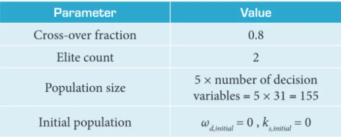
and [ω3d (t1) ... ω3d (tn)] are initialized every 10 s ( ∆t = 10 s or equivalently, n = 10) from the beginning of the fault time (tfault). h erefore, considering ks, the total number of decision variables will be 31. h e considered parameters for GA are presented in Table 3. Other GA parameters are the default values considered in MATLAB® (MathWorks® 2011).
The actuation system consists of 6 thrusters (without considering hardware redundancy), that are placed in opposite directions, and each thruster can produce maximum 50 N variable thrust. h e ef ective moment arm of all thrusters is 1 m along the principal body axis. However, the coni guration of the thrusters is such that (T1− T2), (T3− T4) and (T5 − T6) produce net moments about the i rst, second and third principal axes,
where the superscripts + and – show the positive and negative control torques, respectively.
Note 4: it seems that the thrusters T3, T4, T5and T6pass through the center of gravity. However, as indicated before, they have a moment arm of 1 m along the i rst body axis. h ree important concepts are introduced:
• Initial “fault estimation”: the fault estimation reported by the FDD.
• Worst “fault estimation”: the biggest error of the FDD in providing the fault information. Its value is determined from the initial “fault estimation”, according to the experience or the FDD specii cations. • Real fault: the fault that happens in reality (unknown). h e fault scenario that FDD reports is:
Figure 5. Thruster coni guration. T2 T1
T6
T3 T4
T5
CG
1 2
3 (34)
(35)
(36)
(37)
Parameter Value
Cross-over fraction 0.8
Elite count 2
Population size 5 × number of decision
variables = 5 × 31 = 155
Initial population ωd,initial = 0 , ks,initial = 0
• I n itial “fault estimation”: T5and T6 have lost 99% of their ef ectiveness (â 5 = â 6 = 0.01) and the remaining thrusters are at a good health (â 1 = â 2 = â 3 = â 4 = 1). h e fault occurs at ˆ tfault = 10 s.
• Worst “fault estimation”: based on the experience or the FDD specifications; in the worst case, the following parameters are given: δtfault = 5 s and δa/â = 0.01. h erefore, it can be concluded that, in the worst case, a5 = a6 = 0.0001, i.e. T5and T6 can produce a maximum 0.05 N thrust and the fault occurrence time is tfault = 5 s .
Note 5: it is assumed that the real fault is less severe than the one reported by the worst “fault estimation”. In this case, the controller will show an acceptable performance for less severe, and therefore, a wide range of faults.
Qualitatively, it is assumed that the severity of the faults satisi es the following inequalities:
where S is a quality that represents the severity of the fault; the subscripts w.f.e, r.f and i.f.e stand for worst “fault estimation”, real fault and initial “fault estimation”, respectively.
According to the previous discussion, the proposed method is very conservative, because it considers the worst “fault estimation”. To reduce the adverse ef ects of this assumption, the following quadratic cost function is introduced:
Minimizing this cost function will decrease the adverse ef ects of considering the worst fault estimation. h e consi-dered sample time for integration is 0.1 s. h e problem consists of 2 phases: first, GA tries to satisfy the constraint given by Eq. 34. Then, the result is used as an initial solution to optimize Eq. 39. h e following penalty on cost function is considered:
It was verified that 1,000 s elapsed time is considered as the stopping criterion for the second phase — Intel(R) Core™
2 CPU, [email protected] GHz; MATLAB® (MathWorks® 2011).
To observe the consequences of employing the proposed method, 2 different cases are considered and summarized in Table 4.
Case Fault estimation
1 Considering the initial “fault estimation”
2 Considering the worst “fault estimation”
Table 4. Cases consi dered.
CASe 1
If the initial “fault estimation” is considered (FDD is assumed to report the precise fault information), the results shown in Figs. 6 and 7 will be obtained.
Figure 6. Angular velocities, initial “fault estimation” (case 1).
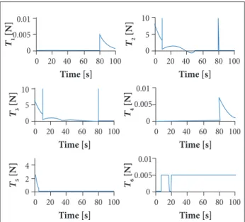
Figure 7. Control inputs, initial “fault estimation” (case 1). 100
80 60
Time [s]
T5 [N] 40 20 0 0 2 4 100 80 60 Time [s] T3 [N] 40 20 0 0 5 10 100 80 60 Time [s] T1 [N] 40 20 0 0 0.005 0.01 100 80 60 Time [s] T6 [N] 40 20 0 0 0.01 0.005 100 80 60 Time [s] T4 [N] 40 20 0 0 0.005 0.01 100 80 60 Time [s] T2 [N] 40 20 0 0 5 10 6 4 2 0
0 10 20 30 40 50 60 70 80 90 100
0 10 20 30 40 50 60 70 80 90 100
0 10 20 30 40 50 60 70 80 90 100
ω ωd ω3 [ d eg /s ] 5 0 – 5 – 10 ω2 [ d eg /s ] 10 5 0 – 5 ω1 [ d eg /s ]
Time [s]
∫ ∫ (38) (39) (40)
Eq. 34 is satisi ed
Figure 6 shows that RG can not make the closed-loop system asymptotically stable, because it assumes the fault scenario reported by the FDD (initial “fault estimation”), which is precise. However, since the real fault is worse than the fault reported by the FDD (initial “fault estimation”), does not converge to the origin. his simulation shows the consequences of considering the initial “fault estimation”. he main conclusion of this simulation is: if the FDD is assumed to report the precise fault information, the response of the controller may not be acceptable.
CASe 2
he result of considering the worst “fault estimation” is illustrated in Fig. 8. he control inputs are illustrated in Fig. 9.
According to Fig. 8, RG can asymptotically stabilize the closed-loop system, when the worst “fault estimation” is considered. A comparison of Figs. 6 and 8 shows the consequences of considering the worst “fault estimation” in the RG design. Clearly, considering the initial “fault estimation” (case 1) can lead to the poor performance of the controller and even to a non-convergent response. On the other hand, if RG is designed for the worst “fault estimation” (case 2), it can cover less severe faults and stabilize the faulty system for a wide range of faults (Note 5).
Since the assumption of worst “fault estimation” is conservative, the response is optimized via minimizing the cost function (Eq. 39). he GA performance is illustrated in Fig. 10. As stated previously, the quadratic cost function has been introduced to reduce the adverse consequences of considering the worst “fault estimation” (maximum fault estimation error). According to Fig. 10, after 14 generations (1,000 s elapsed time), the cost function is reduced from 8,758 to 5,944
100 80 60
Time [s]
T5 [N] 40 20 0 0 2 4 100 80 60 Time [s] T3 [N] 40 20 0 0 5 10 100 80 60 Time [s] T1 [N] 40 20 0 0
0 .0 0 5 0 .0 1
1 0 0 8 0 6 0 Time [s] T6 [N] 4 0 2 0 0 0 0 .0 1
0 .0 0 5
1 0 0 8 0 6 0 Time [s] T4 [N] 4 0 2 0 0 0 2 4
1 0 0 8 0 6 0 Time [s] T2 [N] 4 0 2 0 0 0 5 1 0 0 5,500 6,000 6,500 7,000 7,500 8,000 8,500 9,000
2 4 6 8 10 12 14
Generation J 6 4 2 0
0 10 20 30 40 50 60 70 80 90 100
0 10 20 30 40 50 60 70 80 90 100
0 10 20 30 40 50 60 70 80 90 100
ω ωd ω3 [d eg/s] 20 10 0 –10 ω2 [d eg/s] 10 5 0 ω1 [d eg/s]
Time [s]
(about 32%). his reduction in the cost function decreases the adverse consequences of considering the worst fault estimation.
Figure 8. Angular velocities, worst “fault estimation” (case 2).
Figure 10. Cost function versus generations (1,000 s elapsed time).
Figure 9. Control inputs, worst “fault estimation” (case 2).
DISCUSSION
would be possible to reduce the destructive effects of fault estimation error. A quadratic cost function was defined to reduce the adverse consequences of this conservative assumption (assuming maximum fault estimation error). Therefore, a less sophisticated FDD can be used to satisfy the mission objectives.
AUTHOR’S CONTRIBUTION
Conceptualization, Moradi R; Methodology, Moradi R, Alikhani A, and Fathi Jegarkandi M; Writing – Original Drat, Moradi R and Alikhani A; Writing – Review & Editing, Moradi R, Alikhani A, and Fathi Jegarkandi M.
REFERENCES
Almeida FA (2011) Reference management for fault-tolerant model predictive control. J Guid Control Dynam 34(1):44-56. doi: 10.2514/1.50938
Boussaid B, Aubrun C, Abdelkrim MN (2010) Fault adaptation based on reference governor. Proceedings of the Conference on Control and Fault-Tolerant Systems; Nice, France.
Boussaid B, Aubrun C, Abdelkrim MN (2011) Two-level active fault tolerant control approach. Proceedings of the 8th International Multi-Conference on Systems, Signals and Devices; Sousse, Tunisia.
Boussaid B, Aubrun C, Jiang J, Abdelkrim MN (2014) FTC approach with actuator saturation avoidance based on reference management. International Journal of Robust and Nonlinear Control 24(17):2724-2740. doi: 10.1002/mc.3020
De Boor C (1978) A practical guide to splines. Berlin: Springer.
Fontes FACC (2001) A general framework to design stabilizing nonlinear model predictive controllers. Systems and Control Letters 42(2):127-143. doi: 10.1016/S0167-6911(00)00084-0
Garone E, Di Cairano S, Kolmanovsky IV (2016) Reference and command governors for systems with constraints: A survey on theory and applications. Automatica 75:306-328. doi: 10.1016/j. automatica.2016.08.013
Goldberg DE (1989) Genetic algorithms in search, optimization & machine learning. Reading: Addison-Wesley.
MathWorks® (2011) MATLAB® and SIMULINK®. Natick: MathWorks®.
Miksch T, Gambier A (2011) Fault-tolerant control by using lexicographic multi-objective optimization. Proceedings of the 8th Asian control conference (ASCC); Kaohsiung, Taiwan.
Sidi MJ (2000) Spacecraft dynamics and control: a practical engineering approach. Cambridge: Cambridge University Press.
Sobhani-Tehrani E, Khosravi KH (2009) Fault diagnosis of nonlinear systems using a hybrid approach. Lecture Notes in Control and Information Sciences. Dordrecht; New York: Springer.
Wang D, Jia Y, Jin L, Xu S (2013) Control analysis of an underactuated spacecraft under disturbance. Acta Astronautica 83:44-53. doi: 10.1016/j.actaastro.2012.10.029
Yin S, Xiao B, Ding S, Zhou D (2016) A review on recent development of spacecraft attitude fault tolerant control system. IEEE Trans Ind Electron 63(5):3311-3320. doi: 10.1109/TIE.2016.2530789