www.scielo.br/tema
doi: 10.5540/tema.2018.019.02.0327
A New Scheme for Fault Detection and Classification Applied to DC Motor
L.I. SANTOS1, R.M. PALHARES2, M.F.S.V. D’ANGELO3*, J.B. MENDES3, R.R. VELOSO3and P.Y. EKEL4
Received on October 19, 2017 / Accepted on March 12, 2018
ABSTRACT. This study presents an approach for fault detection and classification in a DC drive system. The fault is detected by a classical Luenberger observer. After the fault detection, the fault classification is started. The fault classification, the main contribution of this paper, is based on a representation which combines the Subctrative Clustering algorithm with an adaptation of Particle Swarm Clustering.
Keywords: Fault Detection and Classification 1, Luenberger Observer 2, Particle Swarm Clustering 3.
1 INTRODUCTION
Fault detection and analysis is a very important strategy that is commonly employed in the in-dustry with the purpose of allowing a cost-effective maintenance policy, keeping productivity standards and ensuring safety. The fault analysis gives support for the design of corrective ac-tions, system redundancies, and safety policies in order to mitigate the effects of a fault [19]. In this paper, a fault diagnosis procedure is divided into two tasks: i) fault detection, indicating the occurrence of some fault in a monitored system; and ii) fault classification, establishing the type and/or location of the fault.
The literature presents several classes of strategies to deal with fault detection and isolation (FDI) [7]. These strategies can be, in general, divided in approaches based on quantitative models [36] and on qualitative models [34], [35].
Considering the quantitative model-based approaches (used for fault detection), many works with different emphases have been published over the past years. Among them, the main ap-proaches focus on knowledge of mathematical models of the plant, and are based on observers
*Corresponding author: Marcos Fl´avio Silveira Vasconcelos D’Angelo – E-mail: [email protected] 1IFNMG Campus Montes Claros – Rua Dois, 300, Village do Lago I, 39404-058, Montes Claros - MG - Brasil. E-mail: [email protected]
2Departamento de Engenharia Eletrˆonica, Universidade Federal de Minas Gerais, Av. Antˆonio Carlos, 6627, 31270-901, Belo Horizonte - MG - Brasil. E-mail: [email protected]
[7], [4], [32], [31], [8], [28]. On the other hand, considering the qualitative model-based ap-proaches (used for fault classification), focusing on the pattern analysis of the historic process data, the main related approaches are: signed directed graphs [24], [9], [2], fault trees [16], fuzzy systems [17],[29], [15], qualitative trend analysis [25], [18], [14], [13], mutual information [38], neural networks [3], [11] (neural networks also can be used as observer [33], [26]), artificial im-mune systems [22], [23], [30], Bayesian networks [39], [37] and the combination of techniques [21], [12].
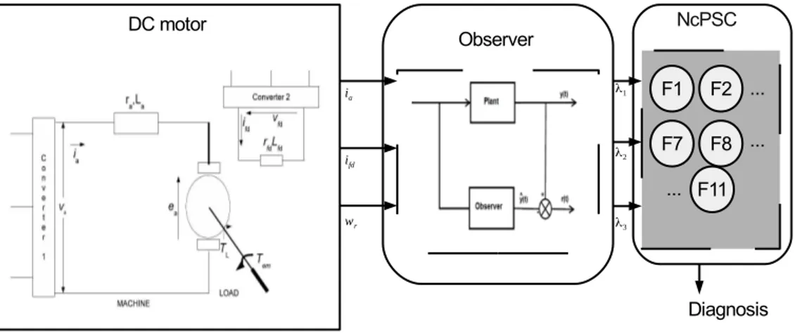
In this paper, an approach for fault detection (first step) and classification (second step) is pre-sented. The classical Luenberger observer is used in the first step, and this information is used for the classification system start. The idea of the second step, the main contribution of this paper, is to deal with the fault classification in a new way, using an adaptation of Particle Swarm Cluster-ing. To illustrate the efficiency of the proposed methodology, the problem of fault detection in a DC Motor Benchmark Model [5] has been solved. An overview of the FDI framework proposed in this paper is illustrated in Figure 1.
Figure 1: Framework for fault detection and classification.
1.1 Contributions
In this paper is proposed an algorithm, adapted fromcPSC ([27]) and denoted as New cPSC (NcPSC), which optimizes the hit rate and the total number of groups (classes) of a data set. It is a supervised algorithm which combines the following functionalities:
• A routine, detailed in subsection 3.2, was developed for generating the initial particle set;
• A particle growing procedure, presented in Algorithm 2, was developed;
• A particle stagnation mechanism, described in Algorithm 3, was implemented.
It is important to note that the proposed functionalities may be adapted in several metaheuristics.
Paper organization.Section 2 presents and analyzes the DC Motor modeling considering the case of different types of faults and the observer design for fault detection. Section 3 describes the adaptive methodology based on Particle Swarm Clustering, the main contribution of this paper, for fault classification. Section 4 shows the new proposed approach applied to the DC motor fault classification problem. Finally, section 5 presents the concluding remarks.
2 LUENBERGER OBSERVER DESIGN FOR DC MOTOR
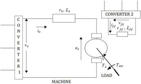
The DC motor benchmark model, evaluated in [5], is descripted as a drive system which consists of two power supplies, controlled static converters, a DC motor and a mechanical load. The system can be represented as shown in Figure 2.
Figure 2: Representation of the DC drive system.
In Figure 2, each variable as the following:
• vais the armature voltage,
• vf dis the field voltage,
• iais the armature current,
• ωrrepresents mechanical rotation speed in rad/s,
• rais the armature resistance,
• Lais the armature inductance,
• rf dis the field resistance,
• Lf dis the field inductance,
• eais the counter electromotive force and is dependent ofLa f d (mutual inductance).
A discrete model for the DC motor is given in (2.1) and presented in [5], whereia=x1,if d=x2 andωr=x3. All state variables are measured, i.e.,y(t) =Ix(t).
x1(k+1) x2(k+1) x3(k+1)
=
a1 a2(k) 0
0 a3 0
a4(k) 0 a5
x1(k) x2(k) x3(k)
+
b1 0 0
0 b2 0
0 0 d1
va(k)
vf d(k)
TL
(2.1)
As the following:a1=a1(ra,La) =e−
ra Lah;
a3=a3(rf d,Lf d) =e −r f dL f dh
; a5=a5(Bm,Jm) =e−
Bm Jmh;
a2(k) =a2(ra,La,rf d,Lf d,x3(k)) =r 1
f dLa−raLf d[La f dLf d(a3−a1)x3(k) +raLf da1−rf dLaa3];
a4(k) =a5(Bm,Jm,x2(k)) =La f d(1−aBm5)x2(k); b1=b1(ra,La) =1−ara1b2=b2(rf d,Lf d) =1r−af d3d1;
d1=d1(Bm,Jm) =−1−aBm5.
where Bm is the coefficient of viscous friction, Jm is the moment of inertia and TL is the
mechanical torque of the load.
x1(k+1)
x2(k+1)
x3(k+1) =
kaaa1f kaaa2f(k) 0
0 ka f da3f 0
a4f(k) 0 a5f
x1(k)
x2(k)
x3(k) +
b1f 0 0
0 b2f 0
0 0 d1f
kaakccava(k) ka f dkcc f dvf d(k)
TL
y1(k)
y2(k)
y3(k) =
kia
f 0 0
0 kif d
f 0
0 0 kωr
f
x1(k)
x2(k)
x3(k)
(2.2)
where: raf =kcarakf vrara, Laf =kcaLaLa, rf df =kc f drf dkf vrf drf d,Lf df =kc f dLf dLf d,Bmf =
kf lBm.
Table 1: Summary of DC motor system faults.
Fault
Fault Type Affected Fault Indicator Parameter
Index Variables Parameters Values
1 Armature converter disconnection ia=0 kaa {0,1}
2 Field converter disconnection if d=0 ka f d. {0,1}
3 Armature converter short circuit va=0 kcca {0,1}
4 Field converter short circuit vf d=0 kcc f d. {0,1}
5 Armature turns short-circuit raandLa kracaandkLaca [0,1]
6 Field turns short-circuit rf dandLf d krf d
c f dandkLf dc f d [0,1]
7 Ventilation system fault raandrf d kf vra andkf vrf d [1,∞)
8 Bearing lubrication fault Bm kf l [1,∞)
9 Armature current sensor fault ia kia
f {0,1}
10 Field current sensor fault if d kif d
f {0,1}
11 Machine speed sensor fault ωr kωr
f {
0,1}
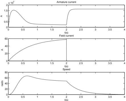
Simulations were made to show some situations of DC motor operation mode. The normal op-eration of the machine and the four faults in the actuators were simulated and the values of the variables are shown in Figs 3 to 7.
0 0.5 1 1.5 2 2.5 3 3.5 4 0
0.5 1 1.5
2x 10
5 Armature current
t(s)
A
0 0.5 1 1.5 2 2.5 3 3.5 4
0 20 40 60 80
Field current
t(s)
A
0 0.5 1 1.5 2 2.5 3 3.5 4
0 20 40 60 80
Speed
t(s)
rad/s
Figure 3: Simulation of the DC motor in normal scenario.
0 0.5 1 1.5 2 2.5 3 3.5 4
0 0.5 1 1.5
2x 10
5 Armature current
t(s)
A
0 0.5 1 1.5 2 2.5 3 3.5 4
0 20 40 60 80
Field current
t(s)
A
0 0.5 1 1.5 2 2.5 3 3.5 4
0 20 40 60 80
Speed
t(s)
rad/s
0 0.5 1 1.5 2 2.5 3 3.5 4 0
0.5 1 1.5
2x 10
5 Armature current
t(s)
A
0 0.5 1 1.5 2 2.5 3 3.5 4
0 20 40 60
Field current
t(s)
A
0 0.5 1 1.5 2 2.5 3 3.5 4
0 20 40 60 80
Speed
t(s)
rad/s
Figure 5: Simulation of the DC motor with disconnection of the field converter.
0 0.5 1 1.5 2 2.5 3 3.5 4
−1 0 1 2x 10
5 Armature current
t(s)
A
0 0.5 1 1.5 2 2.5 3 3.5 4
0 20 40 60 80
Field current
t(s)
A
0 0.5 1 1.5 2 2.5 3 3.5 4
−50 0 50 100
Speed
t(s)
rad/s
0 0.5 1 1.5 2 2.5 3 3.5 4 0
0.5 1 1.5
2x 10
5 Armature current
t(s)
A
0 0.5 1 1.5 2 2.5 3 3.5 4
0 20 40 60
Field current
t(s)
A
0 0.5 1 1.5 2 2.5 3 3.5 4
0 20 40 60 80
Speed
t(s)
rad/s
Figure 7: Simulation of the DC motor with short circuit in the field converter.
2.1 Observer-based fault detection
The aim of the observer-based fault detection method is to generate a residual, used for fault indication. Considering the state space model:
˙
x(t) =Ax(t) +Bu(t) (2.3)
y(t) =Cx(t) (2.4)
whereu(t)is the input ,x(t)is the state andy(t)is the output.
The observer can be designed as follows to provide the system observability:
˙ˆ
x(t) =Axˆ(t) +Bu(t) +Le(t) (2.5)
e(t) =y(t)−Cxˆ(t) (2.6)
ˆ
xis the estimated system state,Lis the matrix of the observer feedback gains that is designed to provide the required performance of the observer ande(t)is the output error.
Replacing (2.6) in (2.5): ˙ˆ
x(t) = [A−LC]xˆ(t) +Bu(t) +Ly(t) (2.7)
The state error is given by:
˙˜
Replacing (2.3) and (2.7) in (2.8):
˙˜
x(t) = [A−LC]x˜(t) (2.9)
The observer design results in:
lim
t→∞˜
x(t) =0
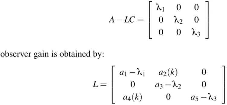
Considering the matrices AandCof the discrete system (2.1) to A−LC, and imposing pole placement to gainLobserver, of the form:
A−LC=
λ1 0 0
0 λ2 0
0 0 λ3
the observer gain is obtained by:
L=
a1−λ1 a2(k) 0
0 a3−λ2 0
a4(k) 0 a5−λ3
Note: for discrete systems, the pole placement ofA−LCis inside unit circle,|λi|<1.
Figure 8 shows residuals for observer gain with λ1=λ2=λ3=0.3 for armature converter disconnection.
3 ADAPTIVE APPROACH FOR FAULT CLASSIFICATION
0 2 4 6 8 10 12 14 16 18 20 −6000
−4000 −2000 0
Residuals
Ia
(A
)
Time (s)
0 2 4 6 8 10 12 14 16 18 20
−1 −0.5 0 0.5 1
If
d (A
)
Time (s)
0 1 2 3 4 5 6 7 8 9 10
−1 −0.5 0 0.5 1
w (rpm)
Time (s)
Figure 8: Residual for observer gain withλ1=λ2=λ3=0.3.
3.1 Concentration level and hit rate
The NcPSC implements a mechanism for growing and pruning particles based on its con-centration level and hit rate. The concon-centration level of a particle p (pcl) is computed
as:
Algorithm 1:Computing CL (p, X).
1 begin
2 pcl←0;
3 foreach Input Data ix∈Xdo
4 ifp is the most similar particle to ixthen
5 pcl←pcl+1; Associateixtop;p.Ix←p.Ix∪ix;
6 end
7 end
8 end
3.2 Generating initial particle set
The initial population plays a key role in terms of convergence rate and may affect the success of an EA in finding high quality or satisfactory solutions [1]. For this reason, theNcPSCalgorithm also implements a simple mechanism for generating initial particles set: Firstly it generates a swarm withN particles. The initial position of each particle is determined using the following mechanism: It calculatesN centroids for the training data set using thesubtractive clustering (SC)method[10].
3.3 Particle growing mechanism
The growing procedure implemented byNcPSCwas proposed for generating new particles and it is based on concentration level and hit rate values of a particle. The proposed method, detailed in Algorithm 2, clones a particle p, resulting in a clone particle p’. A particle pis cloned if its concentration level (p.cl) value is greater thanε1and its hit rate (p.hh) value is less thanγ1- it means that pconcentrates many input data from more than one class (ε1andγ1are parameters ofNcPSC). It is noted that a particle with low hit rate worsens (or deteriorates) the final hit rate of the swarm.
Finally, a simple mutation is performed over a dimension (chosen randomly) of the clone particle. It is expected that clone particles present better hit rates values.
Algorithm 2:Particle growing (p,ε1,γ1).
1 begin
2 ifp.cl>ε1andp.hh<γ1then
3 p’←p.clone();
4 RETURNp’.mutation();
5 end
6 end
3.4 Particle stagnation
A mechanism for particle stagnation was proposed forNcPSCbecause when choosing the most similar particle to the input data, generally more particles move to the crowded regions of the search space. If these crowded regions concentrate several classes, the hit rate values of the attracted particles may be reduced.
Algorithm 3:Particle stagnation (p,ε2,γ2).
1 begin
2 p.stagned←False;
3 ifp.cl>ε2andp.hh>γ2then
4 p.stagned←True;
5 end
6 RETURNp;
7 end
3.5 General structure of theNcPSCalgorithm
The proposedNcPSC, detailed in algorithm 4, is an adaptation ofcPSCalgorithm and it has a set of input parameters presented in the following:
• Number of particles: Variable;
• Input Data: Dataset for clustering;
• ε1=0.60,ε2=0.90,γ1=21 andγ2=15
• ω=0.20;
• Stop condition: 20 (twenty) iterations.
TheNcPSCworks as: Firstly, it generates a swarm withN particles. In the next, the following steps are executed in an ordered and repetitive manner until a termination criterion is found:
• All particles which concentration level value greater thanε2and hit rate value greater than
γ2are marked as stagnated (line 6);
• It identifies the most similar particle from the swarm for each item in the input data. This particle is denoted as the winner particle (Xw). The following operations are applied over
each winner particle (It ismoved):
– Its velocity is updated through expression 3.1:
Vw(t+1) =ωVw(t) +ϕ1⊗(PBestw j(t)−Xw(t))+
ϕ2⊗(GBestj(t)−Xw(t)) +ϕ3⊗(Yj(t)−Xw(t))
(3.1)
whereVw(t)is the particle velocity in iterationt,ω is the inertia component and
– Its position is updated using equation:
Xw(t+1) =Xw(t) +Vw(t+1) (3.2)
– Itspbestandpbestcomponents are updated;
• It removes particles from swarm: All particles with concentration level equal zero are removed from the swarm;
• It clones particles from swarm: All particles with concentration level greater thanε1and with hit rates less thanγ1are cloned.
Algorithm 4:NcPSC algorithm (ID,ε1,γ1,ε2,γ2).
1 begin
2 S←generate initialSwarm(ID);
3 whilestop condition not satisfieddo
4 foreach particle p∈Sdo
5 p.cl←COMPUTE concentration level ofp;p.hh←COMPUTE hit rate ofp;
Particle stagnation(p,ε2,γ2);
6 end
7 foreach item Yj∈IDdo
8 FindXw∈Ssuch thatXwis the most similar particle toYj;
9 ifNOT (Xw.stagned)then
10 UpdateVwusingequation 3.1; UpdateXwusingequation 3.2; Update
Pbestw jeGbestj;
11 end
12 end
13 S.remove particles();
14 foreach particle p∈Sdo
15 Particle growing(p,ε1,γ1);
16 end
17 end
18 end
4 PROPOSED APPROACH APPLIED TO THE FAULT CLASSIFICATION IN DC
MOTOR
• cPSC: The originalcPSCalgorithm proposed in [27];
• cPSCED: A version of cPSC algorithm which implements the Euclidean distance for
similarity measure;
• cPSCPG: An adaptation of cPSC algorithm which develops only the Particle growing
routine;
• cPSCEP: A Version ofcPSCEDwhich combines both the Euclidean distance for similarity
measure and theParticle growingmechanism;
• cPSCPS: An adaptation of cPSCEP algorithm which develops the Particle stagnation
mechanism;
• NcPSC: The proposedNcPSCalgorithm which implements all mentioned functionalities.
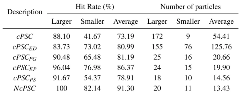
To assess the performance of the developed algorithms they were applied to a clustering problem of a data set with 252 operation points representing 11 (eleven) fault points (Problem with 11 classes). Each algorithm was executed 100 times and each execution performed 20 (twenty) iterations. Some data (Larger, Smaller and average values of hit rate and total of particles) were computed for each algorithm and the obtained results are shown in Table 2.
Table 2: Performance results (Hit rate and Number of particles) for the problem generated by each algorithm.
Description Hit Rate (%) Number of particles
Larger Smaller Average Larger Smaller Average
cPSC 88.10 41.67 73.19 172 9 54.41
cPSCED 83.73 73.02 80.99 155 76 125.76
cPSCPG 90.48 65.48 81.19 25 16 20.66
cPSCEP 96.04 76.98 86.37 24 15 19.90
cPSCPS 91.67 54.37 78.91 18 10 14.56
NcPSC 100 82.14 91.30 20 11 13.43
Some comments about the performance of the 06 algorithms are presented in the following:
• ThecPSCEDand thecPSCalgorithms produced the worst hit rate results. Their greater
• When comparing the three algorithms (cPSCPG,cPSCEP andcPSCPS ), it is noted that
thecPSCEPproduced better hit rate results thancPSCPGandcPSCPS algorithms. On the
other hand, thecPSCPS produced best number of particles (near or equal to the number
of classes) results than the other two algorithms (cPSCPG andcPSCEP algorithms). In
addition, the number of classes found bycPSCEPis a little better thancPSCPG;
• NcPSCwas capable of providing a better clustering than all algorithms. Its hit rate (greater, smaller and average) values better than the others algorithms. Its number of particles (smaller and average) values are better than the results produced by the remaining al-gorithms. It is important to comment that theNcPSCalgorithm found the exact number of classes of the proposed problem. Despite its greater number of classes value is greater than the value found bycPSCPSalgorithm, its average value is closer to the real value than the
average value produced bycPSCPSalgorithm.
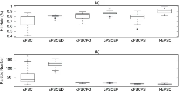
The results generated by the six algorithms are presented in a boxplot perspective shown in Figure 9. Firstly, the hit rate results, illustrated in Figure 9(a), evidence the good performance of thecPSCPG,cPSCEP,cPSCPS andNcPSC algorithms when compared withcPSCandcPSCED
methods.
Also, this perspective emphasizes the good results (both hit rate and particles number) presented by theNcPSC algorithm when compared to the others implementations. The lower boundary of its central box is above the upper boundary of the central box of all others implementations. Figure 9(a) reveals that cPSCED,cPSCEP,cPSCPS andNcPSC (they developed the euclidian
distance as similarity metric) have a more homogeneous behavior thancPSCandcPSCEG
algo-rithms (both implemented the cossin distance as similarity metric). Furthermore, the symmetry is more pronounced incPSCEPandNcPSC implementations. The results generated bycPSCPS
algorithm, which only implements the particle stagnation mechanism, are worser thancPSCEP
results. However, a version which implements all funcionalities (NcPSC algorithm) produced better results than all versions presented in this paper. Also, the total of particles found by each algorithm is presented in a boxplot style (See Figure 9(b)). Again, the figure illustrates the good results produced by algorithms cPSCPG,cPSCEP, cPSCPS andNcPSC andcPSCPG,cPSCEP,
cPSCPS andNcPSC are more homogenic and generated better results thancPSCandcPSCED
algorithms. The total of particles (classes) found by both implementations are closer to the real context than the others algorithms.
5 CONCLUSION
0.4 0.5 0.6 0.7 0.8 0.9 1
cPSC cPSCED cPSCPG cPSCEP cPSCPS NcPSC (a)
Hit Hate (%
)
50 100 150
cPSC cPSCED cPSCPG cPSCEP cPSCPS NcPSC
(b)
Particle Number
Figure 9: Boxplot illustrating the performance of the six implemented algorithms.
ACKNOWLEDGMENT
This work has been supported in part by the Brazilian agencies CNPq and FAPEMIG.
REFERENCES
[1] D. Bajer, G. Martinovi´c & J. Brest. A population initialization method for evolutionary algorithms based on clustering and Cauchy deviates.Expert Systems with Applications,60(2016), 294–310.
[2] T. Boukhobza, F. Hamelin & S. Canitrot. A graph-theoretic approach to fault detection and isolation for structured bilinear systems.International Journal of Control,81(4) (2008), 661–678.
[3] J.M.F. Calado, J. Korbicz, K. Patan, R.J. Patton & J.M.G.S. da Costa. Soft computing approaches to fault diagnosis for dynamic systems.European Journal of Control,7(2-3) (2001), 248–286.
[4] W.M. Caminhas & R.H.C. Takahashi. Dynamic system failure detection and diagnosis employing sliding mode observers and fuzzy neural networks. In “Proceedings of the Joint 9th IFSA and 20th NAFIPS”. Vancouver (2001), pp. 304–309.
[5] W.M. Caminhas & R.H.C. Takahashi. Dynamic system failure detection and diagnosis employing sliding mode observers and fuzzy neural networks. In “Joint nineth IFSA world congress and 20th NAFIPS international conference” (2001), pp. 304–309.
[6] L.N. Castro & S.C.M. Cohen. Data Clustering with Particle Swarms.International Conference on Evolutionary Computation, Proceedings of World Congress on Computational Intelligence, (2006), 1792–1798.
[8] W. Chen & M. Saif. Observer-based strategies for actuator fault detection, isolation and estimation for certain class of uncertain nonlinear systems.IET Control Theoty and Applications,1(6) (2007), 1672–1680.
[9] H. Cheng, M. Nikus & S. Jamsa-Jounela. Fault diagnosis of the paper machine short circulation process using novel dynamic causal digraph reasoning.Journal of Process Control,18(7–8) (2008), 676–691.
[10] S.L. Chiu. Method and software for extracting fuzzy classification rules by subtractive clustering. Biennial Conf. North American Fuzzy Information Processing Soc., (1996), 461–465.
[11] M.F.S.V. D’Angelo & P.P. Costa. Detection of shorted turns in the field winding of turbogenerators using the neural network MLP. In “Proceedings of the IEEE International Conference on Systems, Man, and Cybernetics”. Tucson (2001), pp. 1930–1935.
[12] M.F.S.V. D’Angelo, R.M. Palhares, L.B. Cosme, L.A. Aguiar, F.S. Fonseca & W.M. Caminhas. Fault detection in dynamic systems by a Fuzzy/Bayesian network formulation.Applied Soft Computing,21
(2014), 647–653.
[13] M.F.S.V. D’Angelo, R.M. Palhares, R.H.C. Takahashi & R.H. Loschi. Fuzzy/Bayesian change point detection approach to incipient fault detection.IET Control Theory & Applications,5(4) (2011), 539– 551.
[14] M.F.S.V. D’Angelo, R.M. Palhares, R.H.C. Takahashi, R.H. Loschi, L.M.R. Baccarini & W.M. Cam-inhas. Incipient fault detection in induction machine stator-winding using a fuzzy-Bayesian change point detection approach.Applied Soft Computing,11(1) (2011), 179–192.
[15] K.P. Detroja, , R.D. Gudi & S.C. Patwardhan. A possibilistic clustering approach to novel fault detection and isolation.Journal of Process Control,16(10) (2006), 1055–1073.
[16] Y. Dutuit & A. Rauzy. Approximate estimation of system reliability via fault trees. Reliability Engineering&System Safety,87(2) (2005), 163–172.
[17] S.M. El-Shal & A.S. Morris. A fuzzy expert system for fault detection in statistical process control of industrial processes.IEEE Transactions on Systems, Man and Cybernetics, Part C,30(2) (2000), 281–289.
[18] K.F. Fong, A.P. Loh & W.W. Tan. A frequency domain approach for fault detection. International Journal of Control,81(2) (2008), 264–276.
[19] R. Isermann & P. Balle. Trends in the application of model-based fault detection and diagnosis of technical processes.Control Engineering Practice,5(5) (1997), 707–719.
[20] J. Kennedy & R. Eberhart. Particle Swarm Optimization. Proceedings of IEEE International Conference on Neural Networks (1995), pp. 1942–1948.
[21] C.A. Laurentys, C.H.M. Bomfim, B.R. Menezes & W.M. Caminhas. Design of a pipeline leakage detection using expert system: A novel approach.Applied Soft Computing,11(1) (2011), 1057–1066.
[23] C.A. Laurentys, R.M. Palhares & W.M. Caminhas. A novel Artificial Immune System for fault behavior detection.Expert Systems with Applications,38(11) (2011), 6957–6966.
[24] M.R. Maurya, R. Rengaswamy & V. Venkatasubramanian. A signed directed graph-based system-atic framework for steady-state malfunction diagnosis inside control loops. Chemical Engineering Science,61(6) (2006), 1790–1810.
[25] M.R. Maurya, R. Rengaswamy & V. Venkatasubramanian. Fault diagnosis using dynamic trend anal-ysis: A review and recent developments.Engineering Applications of Artificial Intelligence, 20(2) (2007), 133–146.
[26] K. Patan & T. Parisini. Identification of neural dynamic models for fault detection and isolation: the case of a real sugar evaporation process.Journal of Process Control,15(1) (2005), 67–79.
[27] A.K.F. Prior & L.N. Castro. cPSC: Um algoritmo de enxame construtivo para agrupamento de dados. In “Anais do XVIII Congresso Brasileiro de Autom´atica” (2010), pp. 3300–3307.
[28] V. Puig, A. Stancu, T. Escobet, F. Nejjari, J. Quevedo & R. Patton. Passive robust fault detection using interval observers: Application to the DAMADICS benchmark problem.Control Engineering Practice,14(6) (2006), 621–633.
[29] J. Ragot & D. Maquin. Fault measurement detection in an urban water supply network.Journal of Process Control,16(9) (2006), 887–902.
[30] G.C. Silva, R.M. Palhares & W.M. Caminhas. Immune inspired Fault Detection and Diagnosis: A fuzzy-based approach of the negative selection algorithm and participatory clustering.Expert Systems with Applications,39(16) (2012), 12474–12486.
[31] R.H.C. Takahashi, R.M. Palhares & P.L.D. Peres. Discrete-time Singular Observers: H2/H ∞
Optimality and Unknown Inputs.International Journal of Control,72(6) (1999), 481–492.
[32] R.H.C. Takahashi & P.L.D. Peres. Unknown input observers for uncertain systems: A unifying approach.European Journal of Control,5(2–4) (1999), 261–275.
[33] F.J. Uppal, R.J. Patton & M. Witczak. A neuro-fuzzy multiple-model observer approach to robust fault diagnosis based on the DAMADICS benchmark problem.Control Engineering Practice,14(6) (2006), 699–717.
[34] V. Venkatasubramanian, R. Rengaswamy & S.N. Kavuri. A review of process fault detection and diagnosis – Part II: Qualitative models and search strategies.Computers and Chemical Engineering,
27(3) (2003), 313–326.
[35] V. Venkatasubramanian, R. Rengaswamy, S.N. Kavuri & K. Yin. A review of process fault detection and diagnosis – Part III: Process history based methods.Computers and Chemical Engineering,27(3) (2003), 327–346.
[36] V. Venkatasubramanian, R. Rengaswamy, K. Yin & S.N. Kavuri. A review of process fault detection and diagnosis – Part I: Quantitative model-based methods.Computers and Chemical Engineering,
[37] S. Verron, J. Li & T. Tiplica. Fault detection and isolation of faults in a multivariate process with Bayesian network.Journal of Process Control,20(8) (2010), 902–911.
[38] S. Verron, T. Tiplica & A. Kobi. Fault detection and identification with a new feature selection based on mutual information.Journal of Process Control,18(5) (2008), 479–490.