WAVELET BASED CLASSIFICATION OF VOLTAGE SAG, SWELL & TRANSIENTS

(1)

WAVELET BASED CLASSIFICATION

OF VOLTAGE SAG, SWELL &

TRANSIENTS

Vijay Gajanan Neve*

Assoc. Prof. & HOD of Electrical Engg. Department,

Jagadambha College of Engg. & Tech. YAVATMAL

([email protected])

DR. GAJANAN M. DHOLE

Prof. Electrical Engg. Department,

Shri Sant Gajanan Maharaj

Colleg

e

of Engineering, SHEGAON

( e-mail:[email protected])

Abstract:

When the time localization of the spectral components is needed, the WAVELE TRANSFORM (WT) can be

used to obtain the optimal time frequency representation of the signal. This paper deals with the use of a wavelet

transform to detect and analyze voltage sags, voltage swell and transients. It introduces voltage disturbance

detection approach based on wavelet transform, identifies voltage disturbances, and discriminates the type of

event which has resulted in the voltage disturbance, e.g. either a fault or a capacitor-switching incident.

Feasibility of the proposed disturbance detection approach is demonstrated based on digital time-domain

simulation of a distribution power system using the PSCAD software package, and is implemented using

MATLAB. The developed algorithm has been applied to the 14-buses IEEE system to illustrate its application.

Results are analyzed.

Keywords:

Disturbance detection, Power quality, Voltage Sag, Swell and Transients, Wavelet transform

.

I. Introduction

The both electric utilities and end-users of electric power are becoming increasingly concerned with power

quality. Since the late 1980s the term “power quality” has become the most commonly used buzzword in the

power industry. It covers several types of problems of electricity supply and power system disturbances. Voltage

sags and interruptions, transient overvoltages and harmonics, long-duration voltage variations, wiring and

grounding are all issues related to power quality.

The quality of electrical power supply is widely recognized as one of the most important issues besides the

liberalization of the electricity industry. It is also apparent that too little is known about the quality of existing

power networks. As a result, there are concerted efforts to carry out power quality measurements, not only to

assess the overall quality but also to gather the necessary information for designing improvement measures.

Power quality concerns a subset of electromagnetic phenomena considered under the wider umbrella of

electromagnetic compatibility (EMC), the different phenomena are categorized according to their typical

characteristics of durations, magnitudes, and frequency content. The significance of each category depends on

its impact on other sensitive equipment, which tend to vary from one system to another. Subsequently, the

measurement instruments must be adaptable to cater for the different disturbances. Using data from power

quality studies we examine the variation in power quality at different locations. Our goal is to provide insight on

how much power quality varies by site, what circuit parameters cause the variation,. We focus on the most

common and most problem-causing power quality disturbances—voltage sags, voltage swell and transients

using various power quality indices. Of the many types of power system disturbances that can affect the quality

of supply, voltage sags are known to produce the most devastating impacts on loads. Voltage sags are

characterized by magnitude and duration.

Power system faults cause voltage sag, voltage swell and transients. The frequency of faults depends on many

factors including weather, tree-trimming, and right-of-way maintenance, and age of equipment. The protection

schemes and location of circuit interrupters determine whether a fault causes voltage sag or an interruption, and

the protection system determines the event duration.

(2)

power systems are static, power disturbance waveforms are usually nonstationary and are a periodic under some

circumstances.

Electricite de France (EDF) has been interested for several years in the new signal processing tools used to

detect and measure voltage sags and transient overvoltages. The power quality analysis is a major source of

concern for EDF. Detection and measurement of voltage sags and transient overvoltages must be accurate

enough to determine the cause of the disturbances. A reliable identification of the disturbances enables the

utilities to reinforce the power system.

Many power utilities attempt to continuously monitor power quality by recording disturbance waveforms.

However, the analysis of waveforms recorded is currently based on their visual examination, and because of an

enormous amount of data and a lack of sufficient expertise in power utilities, the task of recognition of

disturbance waveforms is still both difficult and time consuming. Therefore, any attempt to identify or classify

power quality disturbances automatically is very important. Recognition of power quality disturbance

waveforms involves a problem of distinguishing one signal from another. In many situations, power utilities

cannot provide sufficient amount of data .The amount of data collected is often very large, Most of the collected

data is often stored in a mass storage system without real-time analysis or until a complaint or a significant

disturbance occurs. It is therefore desired that every incoming waveform be automatically identified and

tabulated into specific disturbance categories. Wavelet transform (WT) is a recent signal processing tool used in

power, quality analysis, provides an understandable transient signal representation corresponding to a

time-frequency plane. This plane gives time and time-frequency related information relating to the analyzed signal.

Therefore, the WT leads to accurate frequency resolution and poor time location at low frequency. Reciprocally,

the WT provides accurate time location and bad frequency resolution at high frequency. This characteristic is

appropriate for real signals such as voltage sags and transient overvoltages. Time-frequency planes are also

meaningful signatures of each kind of disturbances providing time and frequency characteristics. Detecting and

characterizing voltage sags and transients are tested over a set of records representing real disturbances [1].

This paper mainly concentrates on describing the principles of the disturbance detection scheme is evaluated

based on simulation of a large number of faults and capacitor-switching incidents in a power distribution

system. The PSCAD program is used for the simulation studies. This paper is organized as follows. Section II

outlines the Background, Section III describes the System under study, Section IV shows the graphical results

for various cases considered separately and Section V draws the conclusions.

II. Background

To improve power quality with adequate solutions, it is necessary to know what kinds of disturbances

occurred. A measurement system able to automatically detect, characterize, and classify disturbances on

electrical lines is therefore required. Simulation studies have been carried out for single line to ground faults.

Voltage sags is defined as “a decrease to between 0.1 and 0.9 p.u. in rms voltage at the power frequency for a

duration of 0.5 cycle to 1 min” or it may be defined as Voltage sags are power system events that present a

temporary decrease in the rms voltage magnitude in one or more phases. Voltage sags are also called as voltage

dips. They are one of the most concerned power quality disturbances in power systems. voltage sags are

characterized by its magnitude and duration. The magnitude is defined as the percentage of the remaining

voltage during the sag. In this case, the duration of sag is the time between the sag commencement and end. The

magnitude and the duration of voltages sag in use in this paper are the remaining bus voltage during the fault

and the required time to clear the fault by primary protection, respectively. Magnitude and duration are the main

characteristics of voltage sags, and they have been used for the development of the equipment’s compatibility

charts and indices. In addition to these, the other characteristics such as unbalanced voltage sags, phase angle

shifts, the point on the wave of initiation and recovery, and waveform distortion have been found to influence

significantly the equipment’s sensitivity to the voltage sags. A three-phase short circuit or a large motor starting

can produce symmetrical sags whereas single-line-to-ground, phase-to-phase, and two-phase-to-ground faults

can cause asymmetrical sags. The majority of faults in the power systems are the single line-to-ground faults,

and consequently result in the unbalanced voltage sags. The sources for voltage sags are usually system faults,

heavy load switching, and large motor starting. Sags can propagate long distance from the source location and

affect customers in large areas. Over the past many years, research work in voltage sag diagnosis has been

focused on developing protocols and systems to measure the disturbance. Little work has been reported on

locating the origins of voltage sags. With the deregulation of power industry, utilities have become increasingly

interested in quantifying the responsibilities for power quality problems, with voltage sag as the most prominent

concern. As a result, research on how to detect sag source direction has become an important topic recently. In

spite of various efforts, there is still no reliable and technically sound method available for locating sag sources.

(3)

voltage sags from the original fault locations to the different customer buses. A voltage dip at the terminals of

equipment may lead to maloperations of the equipment. Most maloperations are associated with voltage dips

due to faults. One of the causes of maloperations is the sudden increase in voltage upon fault clearing.

Voltage dips due to faults are the most severe ones and therefore are of major concern. They cause problems

to a large number of customers as they propagate in the system. The magnitude of fault-induced voltage dips at

a certain point in the system depends mainly on the type and the resistance of the fault, the distance to the fault

and the system configuration. Their duration depends on the type of protection that is used and varies between

less than half a cycle (for a fuse) to a few seconds. Faults are either symmetrical (three-phase or

three-phase-to-ground faults) or nonsymmetrical (single-phase or double-phase or double-phase-to-three-phase-to-ground faults). Depending

on the type of fault, the magnitudes of the voltages of the three phases are equal (symmetrical fault) or unequal

(nonsymmetrical) [2].

Four basic fault types (line-to-ground L-G, line-to-line L-L, ground L-L-G, and

line-to-line-to-line L-L-L) are initiated at every bus in the network. Related voltage sags, caused by these faults, are then

“followed” during the propagation to the particular bus of interest. In this way, a “voltage sag profile” at the bus

of interest is obtained. The voltage sag profile shows the three-phase voltage magnitudes as they occur at the bus

of interest as the consequence of four fault types initiated at all buses in the network. [3].

The characteristics of each disturbance, e.g. a fault, depend on several factors, for example type of the event,

e.g. single-phase-to-ground or phase-to-phase fault, location of the event, time instant of the event, and

network configuration. The basic uncertainty factors recognized in the assessment of voltage sags are as

follows:

a) Fault type: System faults considered in this paper are; three-phase, line, single- and double

line-to-ground faults. The probabilities associated with fault types depend upon the operating voltage, weather

conditions, etc. and can vary from system to system. The probability of occurrence of each of these fault types

should be obtained from actual system data and statistics of fault incidence.

b) Fault location: The resulting severity of a given fault tends to diminish as the distance between the fault

location and the generating buses increases. Faults at generator buses are the most severe faults in the system.

The location of the fault is probabilistic and, therefore, can be represented by a probability distribution of fault

occurrence.

c) Fault impedance: Ground faults on lines usually result from flashover of the insulators due to lightning

induction or failure of the insulators. The current path for ground faults includes the arc, tower impedance and

the impedance between the tower foundation and earth (tower footing resistance). When used, ground wires

provide a parallel path to the earth return. Arcs are resistive in nature, while tower and ground wires are

complex impedances and tower footing impedance is essentially resistive. A typical value of the arc resistance is

1 or 2 ohms. Tower footing resistance at various towers can run from less than 1 to several hundred ohms. With

so many variables, it is quite difficult to represent the fault resistance with any degree of certainty. It is a

common assumption that the fault impedance is totally resistive.

Voltage swell as defined by IEEE Standard 1159-1995, IEEE Recommended Practice for Monitoring Electric

Power Quality, is an

increase in root mean square (RMS) voltage at the power frequency for durations from 0.5

cycles to 1 minute. Typical magnitudes are between 1.1 and 1.8 pu.

As with sags, swells are usually associated with system fault conditions, but they are much less common than

voltage sags. A swell can occur due to a single line-to-ground fault on the system resulting in a temporary

voltage rise on the unfaulted phases. Swells can also be caused by switching off a large load, switching on a

large capacitor bank etc.

Swells are characterized by their magnitude (RMS value) and duration. The severity of a voltage swell during

a fault condition is a function of the fault location, system impedance, and grounding.

The transient is due to the instant of voltage recovery corresponds to the instant of fault clearing. The

non-zero signal before the start of the event is due to the method for extracting the transient being non-ideal. An

appropriate high-pass filter would remove the harmonic distortion but would also remove a significant part of

the transient as its main frequency components are around a few hundred Hertz. Also, the original waveform

and the extracted transients for the three phases are shown.

(4)

Wavelet Toolbox™ software extends the MATLAB® technical computing environment with graphical tools

and command-line functions for developing wavelet-based algorithms for the analysis, synthesis, denoising, and

compression of signals and images. Wavelet analysis provides more precise information about signal data than

other signal analysis techniques, such as Fourier. The Wavelet Toolbox supports the interactive exploration of

wavelet properties and applications. It is useful for speech and audio processing, image and video processing,

biomedical imaging, and 1-D and 2-D applications in communications and geophysics The Wavelet transform is

a transform of this type. It provides the time-frequency representation. Wavelet transform is capable of

providing the time and frequency information simultaneously, hence giving a time-frequency representation of

the signal.

The wavelet transforms associated with fast electromagnetic transients are typically non-periodic signals,

which contain both high-frequency oscillations and localized impulses superimposed on the power frequency

and its harmonics. If signals are altered in a localized time instant, the entire frequency spectrum can be

affected. To reduce the effect of non-periodic signals on the DFT, the short-time Fourier transform (STFT) is

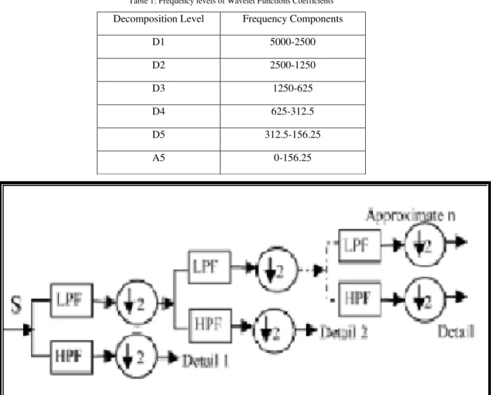
used. It assumes local periodicity within a continuously translated time window. Fig.1 illustrates the

implementation procedure of a Discrete WT (DWT), in which S is the original signal; LPF and HPF are the

low-pass and high-low-pass filters respectively. At the first stage an original signal is divided in to two halves of the

frequency bandwidth, and sent to both LPF and HPF. Then the output of LPF is further cut in half of the

frequency bandwidth and then sent to the second stage, this procedure is repeated until the signal is decomposed

to a pre-defined certain level. If the original signal were being sampled at Fs Hz, the highest frequency that the

signal could contain, from Nyquist’s theorem, would be Fs/2 Hz. This frequency would be seen at the output of

the high pass filter, which is the first detail 1, similarly, the band of frequencies between Fs/4 and Fs/8 would be

captured in detail 2, and so on. The sampling frequency in this paper is taken to be 10 kHz and Table 1 shows

the frequency levels of the wavelet function coefficients.

Table 1: Frequency levels of Wavelet Functions Coefficients

Decomposition Level

Frequency Components

D1 5000-2500

D2 2500-1250

D3 1250-625

D4 625-312.5

D5 312.5-156.25

A5 0-156.25

(5)

III. System under study

The IEEE Test System was used in the studies reported in this paper. Fig.2 shows 14-bus system is used for

the test example. The system data is given in Appendix A. At each observation location, harmonic and voltage

fluctuation phenomena are considered, System bus voltages are calculated by using the fault calculations

program written using MATLAB. Voltage sag magnitudes at the network buses are calculated for symmetrical

and asymmetrical faults out of these 14 buses, Eight network buses (i.e., buses 4, 7, 9, 10, 11, 12, 13, and 14)

are selected arbitrarily as the buses of interest

.

Out of these eight buses, the first six are 11-kV buses whereas the

last two are at the 33-kV level.

The objective is to monitor the voltage at the 9

th

bus and identify voltage disturbances in various four cases

such as, single line to ground fault (solidly grounded), single line to ground fault (resistance grounding with

Rf=10

Ω

),.Sudden load applied & Capacitor switching. The logic is to discriminate between voltage

disturbances due to faults and capacitor-switching incidents. This information may be used to take proper

countermeasures to maintain the bus voltage during system faults within prescribed limits.

The emphasis here is to develop a methodology to incorporate the uncertainty involved with the equipment

sensitivity. Therefore, in order to simplify calculations, in case of the asymmetrical sags Due to space

limitations, results obtained only at affected buses are discussed here [4].

Fig. 2. IEEE 14 Bus System

IV. Results and Discussion

In order to analyze the operation of the proposed computer simulations with power system computer aided

design PSCAD were performed. Power disturbance

Data of 14 Bus System have been recorded. The data were

obtained from a

power system software PSCAD The power circuit is modeled as a three-phase four-wire system

with a nonlinear load, in PSCAD software. The length of each signal is 15000 samples for 0.8 s [6].

(6)

calculations, due to space limitations, results obtained only at affected eight buses are shown (i.e. bus No.

4,7,9,10,11,12,13,14). The objective is to monitor the voltage at the 9

th

(select arbitrarily) bus and identify

voltage disturbances in various four cases such as, single line to ground fault (solidly grounded), single line to

ground fault (resistance grounding with Rf=10

Ω

), Sudden load applied & Capacitor switching are as under.

A)

Single line to ground Fault without considering fault resistance i.e solidly grounded

The experimental study has been carried out for a single-phase to ground fault without considering fault

resistance i.e solidly grounded event. Now suppose that a single line to ground fault without considering fault

resistance occurs on bus No. 9 at phase A and is cleared after a period of time.

In all of the investigations reported in this paper, the bus voltage at a faulted phase is zero. Moreover, in the

case of unsymmetrical faults, the voltage sag magnitude is the lowest value of all phases. It gives sample

simulation results of the voltage sag magnitude at selected buses for single line to ground faults on the 9

th

bus. It

can be seen from this Fig. 3-10 that buses near to a fault experience severe voltage sag. The influence of the

distance to the fault on the sag magnitude is demonstrated graphically in Fig. 3-10 for the 14 bus system. As

can be seen, the voltage drops below 90% for a large part of the network. Such a fault thus has the potential to

cause sag-related equipment problems for a large number of customers.. As expected, it can be seen that the

voltage sag is more severe for faults close to the customer bus.. It can be seen from this figure that generator

buses experience lower voltage sags than load buses. It can also be seen that bus 9 experiences the highest

voltage sag as compared to other buses and also we have seen that there will be no any affect on bus no.

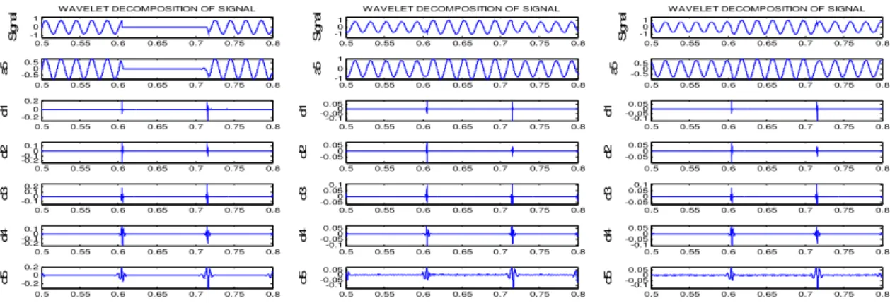
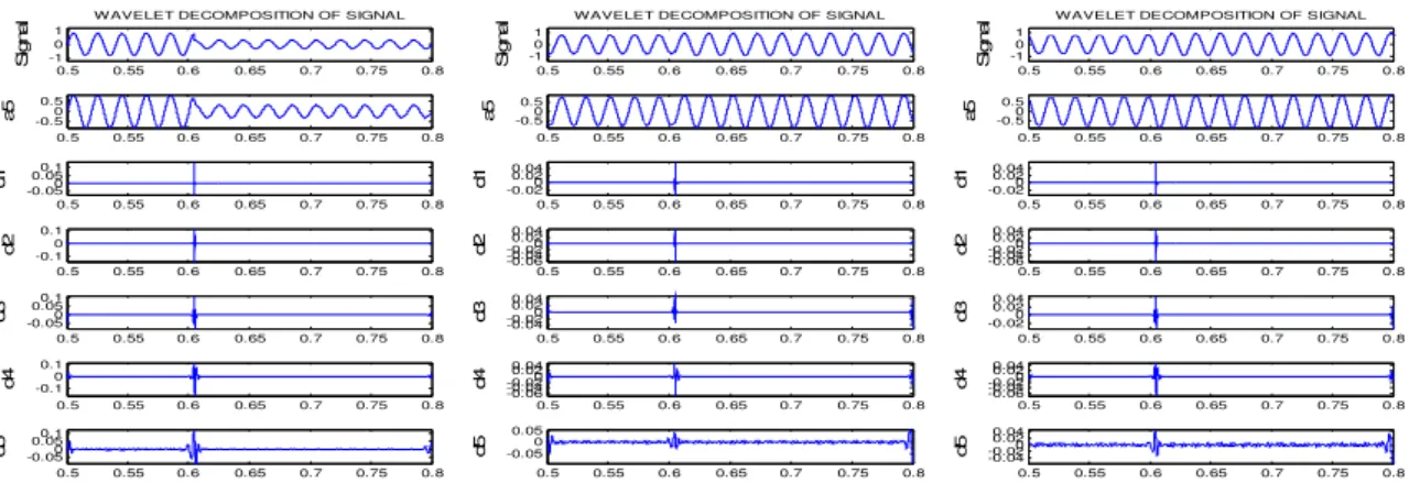
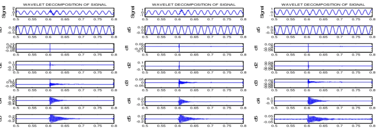
1,2,3,5,6,and 8. Fig.3 clearly shows that at bus No. 9 on phase A fault record from a single-phase to ground

without considering fault resistance of three-phase power System,. are the voltage of phase a, b, and c,

respectively, there will more affect, such as sag seen on faulted phase and swell occurs on unfaulted phases i.e.

phase b and phase c. The instant of voltage recovery corresponds to the instant of fault clearing.

0.5 0.55 0.6 0.65 0.7 0.75 0.8 -1

0 1

S

igna

l

W AVELET DECOMPOSITION OF SIGNAL

0.5 0.55 0.6 0.65 0.7 0.75 0.8 -0.50

0.5

a5

0.5 0.55 0.6 0.65 0.7 0.75 0.8 -0.2

0 0.2

d1

0.5 0.55 0.6 0.65 0.7 0.75 0.8 -0.2

-0.10 0.1

d2

0.5 0.55 0.6 0.65 0.7 0.75 0.8 -0.10

0.1 0.2

d3

0.5 0.55 0.6 0.65 0.7 0.75 0.8 -0.2

-0.10 0.1

d4

0.5 0.55 0.6 0.65 0.7 0.75 0.8 -0.2

0 0.2

d5

0.5 0.55 0.6 0.65 0.7 0.75 0.8 -10

1

S

igna

l

0.5 0.55 0.6 0.65 0.7 0.75 0.8 -1

0 1

a5

0.5 0.55 0.6 0.65 0.7 0.75 0.8 -0.1

-0.050 0.05

d1

0.5 0.55 0.6 0.65 0.7 0.75 0.8 -0.050

0.05

d2

0.5 0.55 0.6 0.65 0.7 0.75 0.8 -0.050

0.050.1

d3

0.5 0.55 0.6 0.65 0.7 0.75 0.8 -0.1

-0.050 0.05

d4

0.5 0.55 0.6 0.65 0.7 0.75 0.8 -0.1

-0.050 0.05

d5

0.5 0.55 0.6 0.65 0.7 0.75 0.8 -10

1

S

igna

l

WAVELET DECOMPOSITION OF SIGNAL

0.5 0.55 0.6 0.65 0.7 0.75 0.8 -0.50

0.5

a5

0.5 0.55 0.6 0.65 0.7 0.75 0.8 -0.1

-0.050 0.05

d1

0.5 0.55 0.6 0.65 0.7 0.75 0.8 -0.050

0.05

d2

0.5 0.55 0.6 0.65 0.7 0.75 0.8 -0.050

0.050.1

d3

0.5 0.55 0.6 0.65 0.7 0.75 0.8 -0.1

-0.050 0.05

d4

0.5 0.55 0.6 0.65 0.7 0.75 0.8 -0.1

-0.050 0.05

d5

Fig. 3. At bus No. 9 fault record from a single-phase to ground of three-phase power System,. are the voltage of phase a, b, and c,

respectively. The fault occurred on phase A at Bus No. 9 (Solidly grounded)

0.5 0.55 0.6 0.65 0.7 0.75 0.8 -1

0 1

S

ignal

0.5 0.55 0.6 0.65 0.7 0.75 0.8 -0.50

0.5

a5

0.5 0.55 0.6 0.65 0.7 0.75 0.8 -50

5 x 10-3

d1

0.5 0.55 0.6 0.65 0.7 0.75 0.8 -50

5 10 15x 10

-3

d2

0.5 0.55 0.6 0.65 0.7 0.75 0.8 -0.05

0 0.05

d3

0.5 0.55 0.6 0.65 0.7 0.75 0.8 -0.020

0.02

d4

0.5 0.55 0.6 0.65 0.7 0.75 0.8 -0.050

0.050.1

d5

0.5 0.55 0.6 0.65 0.7 0.75 0.8 -1

0 1

S

ignal

0.5 0.55 0.6 0.65 0.7 0.75 0.8 -0.5

0 0.5

a5

0.5 0.55 0.6 0.65 0.7 0.75 0.8 -2

-10 1

x 10-3

d1

0.5 0.55 0.6 0.65 0.7 0.75 0.8 -6

-4 -20 2

x 10-3

d2

0.5 0.55 0.6 0.65 0.7 0.75 0.8 -0.02

0 0.02

d3

0.5 0.55 0.6 0.65 0.7 0.75 0.8 -20

-100 x 10-3

d4

0.5 0.55 0.6 0.65 0.7 0.75 0.8 -0.04

-0.020 0.02

d5

0.5 0.55 0.6 0.65 0.7 0.75 0.8 -1

0 1

S

ignal

0.5 0.55 0.6 0.65 0.7 0.75 0.8 -0.50

0.5

a5

0.5 0.55 0.6 0.65 0.7 0.75 0.8 -50

5 x 10-3

d1

0.5 0.55 0.6 0.65 0.7 0.75 0.8 -5

0 5

x 10-3

d2

0.5 0.55 0.6 0.65 0.7 0.75 0.8 -0.020

0.02

d3

0.5 0.55 0.6 0.65 0.7 0.75 0.8 -0.010

0.01

d4

0.5 0.55 0.6 0.65 0.7 0.75 0.8 -0.04

-0.020 0.02

d5

(7)

0.5 0.55 0.6 0.65 0.7 0.75 0.8 -1 0 1

S

ig

nal

0.5 0.55 0.6 0.65 0.7 0.75 0.8 -0.50

0.5

a5

0.5 0.55 0.6 0.65 0.7 0.75 0.8 -0.10

0.1

d1

0.5 0.55 0.6 0.65 0.7 0.75 0.8 -0.1

0 0.1

d2

0.5 0.55 0.6 0.65 0.7 0.75 0.8 -0.050.050

0.1

d3

0.5 0.55 0.6 0.65 0.7 0.75 0.8 -0.10

0.1

d4

0.5 0.55 0.6 0.65 0.7 0.75 0.8 -0.10

0.1

d5

0.5 0.55 0.6 0.65 0.7 0.75 0.8 -1 0 1

S

ig

nal

0.5 0.55 0.6 0.65 0.7 0.75 0.8 -0.50

0.5

a5

0.5 0.55 0.6 0.65 0.7 0.75 0.8 -0.050

0.05

d1

0.5 0.55 0.6 0.65 0.7 0.75 0.8 -0.05

0 0.05

d2

0.5 0.55 0.6 0.65 0.7 0.75 0.8 -0.04

-0.020.020.040 0.06

d3

0.5 0.55 0.6 0.65 0.7 0.75 0.8 -0.050

0.05

d4

0.5 0.55 0.6 0.65 0.7 0.75 0.8 -0.050

0.05

d5

0.5 0.55 0.6 0.65 0.7 0.75 0.8 -1 0 1

S

ig

nal

0.5 0.55 0.6 0.65 0.7 0.75 0.8 -0.50

0.5

a5

0.5 0.55 0.6 0.65 0.7 0.75 0.8 -0.050

0.05

d1

0.5 0.55 0.6 0.65 0.7 0.75 0.8 -0.05

0 0.05

d2

0.5 0.55 0.6 0.65 0.7 0.75 0.8 -0.04

-0.020.020.040 0.06

d3

0.5 0.55 0.6 0.65 0.7 0.75 0.8 -0.050

0.05

d4

0.5 0.55 0.6 0.65 0.7 0.75 0.8 -0.050

0.05

d5

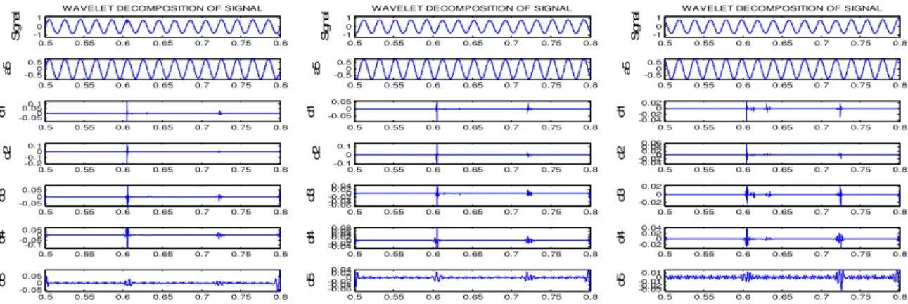
Fig. 5. At bus No. 7 fault record from a single-phase to ground of three-phase power System,. are the voltage of phase a, b, and c,

respectively. The fault occurred on phase A at Bus No. 9 (Solidly grounded)

0.5 0.55 0.6 0.65 0.7 0.75 0.8 -1

0 1

S

ign

al

0.5 0.55 0.6 0.65 0.7 0.75 0.8 -0.50

0.5

a5

0.5 0.55 0.6 0.65 0.7 0.75 0.8 -0.2

-0.10 0.1

d1

0.5 0.55 0.6 0.65 0.7 0.75 0.8 -0.10

0.1

d2

0.5 0.55 0.6 0.65 0.7 0.75 0.8 -0.10

0.1 0.2

d3

0.5 0.55 0.6 0.65 0.7 0.75 0.8 -0.2

-0.10 0.1

d4

0.5 0.55 0.6 0.65 0.7 0.75 0.8 -0.2

-0.10 0.1

d5

0.5 0.55 0.6 0.65 0.7 0.75 0.8 -10

1

S

ign

al

0.5 0.55 0.6 0.65 0.7 0.75 0.8 -0.50

0.5

a5

0.5 0.55 0.6 0.65 0.7 0.75 0.8 -0.1

-0.050 0.05

d1

0.5 0.55 0.6 0.65 0.7 0.75 0.8 -0.050

0.05

d2

0.5 0.55 0.6 0.65 0.7 0.75 0.8 -0.050

0.05

d3

0.5 0.55 0.6 0.65 0.7 0.75 0.8 -0.050

0.05

d4

0.5 0.55 0.6 0.65 0.7 0.75 0.8 -0.1

-0.050 0.05

d5

0.5 0.55 0.6 0.65 0.7 0.75 0.8 -10

1

S

ign

al

0.5 0.55 0.6 0.65 0.7 0.75 0.8 -0.50

0.5

a5

0.5 0.55 0.6 0.65 0.7 0.75 0.8 -0.1

-0.050 0.05

d1

0.5 0.55 0.6 0.65 0.7 0.75 0.8 -0.050

0.05

d2

0.5 0.55 0.6 0.65 0.7 0.75 0.8 -0.050

0.05

d3

0.5 0.55 0.6 0.65 0.7 0.75 0.8 -0.050

0.05

d4

0.5 0.55 0.6 0.65 0.7 0.75 0.8 -0.1

-0.050 0.05

d5

Fig. 6. At bus No. 10 fault record from a single-phase to ground of three-phase power System,. are the voltage of phase a, b, and c,

respectively. The fault occurred on phase A at Bus No. 9 (Solidly grounded)

0.5 0.55 0.6 0.65 0.7 0.75 0.8 -1

0 1

S

ignal

0.5 0.55 0.6 0.65 0.7 0.75 0.8 -0.50

0.5

a5

0.5 0.55 0.6 0.65 0.7 0.75 0.8 -0.1

-0.050 0.05

d1

0.5 0.55 0.6 0.65 0.7 0.75 0.8 -0.050

0.05

d2

0.5 0.55 0.6 0.65 0.7 0.75 0.8 -0.050

0.050.1

d3

0.5 0.55 0.6 0.65 0.7 0.75 0.8 -0.1

-0.050 0.05

d4

0.5 0.55 0.6 0.65 0.7 0.75 0.8 -0.1

0 0.1

d5

0.5 0.55 0.6 0.65 0.7 0.75 0.8 -10

1

S

ignal

0.5 0.55 0.6 0.65 0.7 0.75 0.8 -0.50

0.5

a5

0.5 0.55 0.6 0.65 0.7 0.75 0.8 -0.04

-0.020 0.02

d1

0.5 0.55 0.6 0.65 0.7 0.75 0.8 -0.04

-0.020 0.02

d2

0.5 0.55 0.6 0.65 0.7 0.75 0.8 -0.020

0.02 0.04

d3

0.5 0.55 0.6 0.65 0.7 0.75 0.8 -0.04

-0.020 0.02

d4

0.5 0.55 0.6 0.65 0.7 0.75 0.8 -0.06

-0.04 -0.020.020

d5

0.5 0.55 0.6 0.65 0.7 0.75 0.8 -10

1

S

ignal

0.5 0.55 0.6 0.65 0.7 0.75 0.8 -0.50

0.5

a5

0.5 0.55 0.6 0.65 0.7 0.75 0.8 -0.04

-0.020 0.02

d1

0.5 0.55 0.6 0.65 0.7 0.75 0.8 -0.04

-0.020 0.02

d2

0.5 0.55 0.6 0.65 0.7 0.75 0.8 -0.020

0.02 0.04

d3

0.5 0.55 0.6 0.65 0.7 0.75 0.8 -0.04

-0.020 0.02

d4

0.5 0.55 0.6 0.65 0.7 0.75 0.8 -0.04

-0.020 0.02

d5

Fig. 7. At bus No. 11 fault record from a single-phase to ground of three-phase power System,. are the voltage of phase a, b, and c,

respectively. The fault occurred on phase A at Bus No. 9 (Solidly grounded)

0.5 0.55 0.6 0.65 0.7 0.75 0.8 -1

0 1

S

ignal

0.5 0.55 0.6 0.65 0.7 0.75 0.8 -0.50

0.5

a5

0.5 0.55 0.6 0.65 0.7 0.75 0.8 -0.02

-0.010 0.01

d1

0.5 0.55 0.6 0.65 0.7 0.75 0.8 -0.010

0.01

d2

0.5 0.55 0.6 0.65 0.7 0.75 0.8 -0.05

0 0.05

d3

0.5 0.55 0.6 0.65 0.7 0.75 0.8 -0.020

0.02

d4

0.5 0.55 0.6 0.65 0.7 0.75 0.8 -0.050

0.050.1

d5

0.5 0.55 0.6 0.65 0.7 0.75 0.8 -1

0 1

S

ignal

0.5 0.55 0.6 0.65 0.7 0.75 0.8 -0.50

0.5

a5

0.5 0.55 0.6 0.65 0.7 0.75 0.8 -10-5

0 5x 10

-3

d1

0.5 0.55 0.6 0.65 0.7 0.75 0.8 -50

5x 10

-3

d2

0.5 0.55 0.6 0.65 0.7 0.75 0.8 -0.020

0.02

d3

0.5 0.55 0.6 0.65 0.7 0.75 0.8 -20

-100 x 10-3

d4

0.5 0.55 0.6 0.65 0.7 0.75 0.8 -0.06

-0.04 -0.020 0.02

d5

0.5 0.55 0.6 0.65 0.7 0.75 0.8 -1

0 1

S

ignal

0.5 0.55 0.6 0.65 0.7 0.75 0.8 -0.50

0.5

a5

0.5 0.55 0.6 0.65 0.7 0.75 0.8 -10-5

0 5x 10

-3

d1

0.5 0.55 0.6 0.65 0.7 0.75 0.8 -50

5x 10

-3

d2

0.5 0.55 0.6 0.65 0.7 0.75 0.8 -0.02

0 0.02

d3

0.5 0.55 0.6 0.65 0.7 0.75 0.8 -0.010

0.01

d4

0.5 0.55 0.6 0.65 0.7 0.75 0.8 -0.04

-0.020 0.02

d5

(8)

0.5 0.55 0.6 0.65 0.7 0.75 0.8 -1

0 1

S

ig

nal

0.5 0.55 0.6 0.65 0.7 0.75 0.8 -0.50

0.5

a5

0.5 0.55 0.6 0.65 0.7 0.75 0.8 -0.04

-0.020 0.02

d1

0.5 0.55 0.6 0.65 0.7 0.75 0.8 -0.020

0.02

d2

0.5 0.55 0.6 0.65 0.7 0.75 0.8 -0.05

0 0.05

d3

0.5 0.55 0.6 0.65 0.7 0.75 0.8 -0.020

0.02

d4

0.5 0.55 0.6 0.65 0.7 0.75 0.8 -0.050

0.050.1

d5

0.5 0.55 0.6 0.65 0.7 0.75 0.8 -1

0 1

S

ig

nal

0.5 0.55 0.6 0.65 0.7 0.75 0.8 -0.50

0.5

a5

0.5 0.55 0.6 0.65 0.7 0.75 0.8 -0.010

0.01

d1

0.5 0.55 0.6 0.65 0.7 0.75 0.8 -0.01

0 0.01

d2

0.5 0.55 0.6 0.65 0.7 0.75 0.8 -0.020

0.02

d3

0.5 0.55 0.6 0.65 0.7 0.75 0.8 -0.02

-0.010 0.01

d4

0.5 0.55 0.6 0.65 0.7 0.75 0.8 -0.06

-0.04 -0.020 0.02

d5

0.5 0.55 0.6 0.65 0.7 0.75 0.8 -1

0 1

S

ig

nal

0.5 0.55 0.6 0.65 0.7 0.75 0.8 -0.50

0.5

a5

0.5 0.55 0.6 0.65 0.7 0.75 0.8 -0.010

0.01

d1

0.5 0.55 0.6 0.65 0.7 0.75 0.8 -0.01

0 0.01

d2

0.5 0.55 0.6 0.65 0.7 0.75 0.8 -0.020

0.02

d3

0.5 0.55 0.6 0.65 0.7 0.75 0.8 -0.01

0 0.01

d4

0.5 0.55 0.6 0.65 0.7 0.75 0.8 -0.04

-0.020 0.02

d5

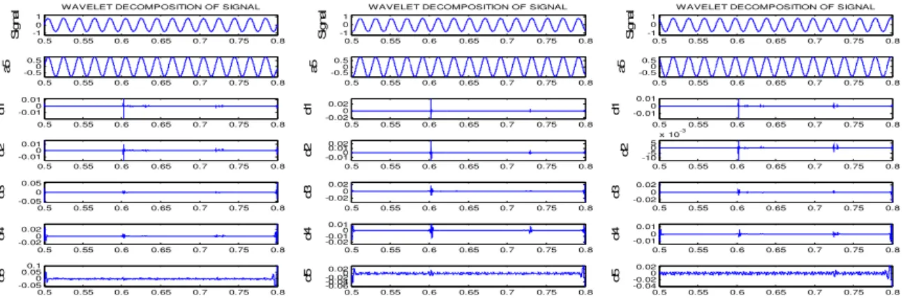
Fig. 9. At bus No. 13 fault record from a single-phase to ground of three-phase power System,. are the voltage of phase a, b, and c,

respectively. The fault occurred on phase A at Bus No. 9 (Solidly grounded)

0.5 0.55 0.6 0.65 0.7 0.75 0.8 -1

0 1

S

ign

al

0.5 0.55 0.6 0.65 0.7 0.75 0.8 -0.50

0.5

a5

0.5 0.55 0.6 0.65 0.7 0.75 0.8 -0.10

0.1

d1

0.5 0.55 0.6 0.65 0.7 0.75 0.8 -0.1

0 0.1

d2

0.5 0.55 0.6 0.65 0.7 0.75 0.8 -0.050.050

0.1 0.15

d3

0.5 0.55 0.6 0.65 0.7 0.75 0.8 -0.10

0.1

d4

0.5 0.55 0.6 0.65 0.7 0.75 0.8 -0.10

0.1

d5

0.5 0.55 0.6 0.65 0.7 0.75 0.8 -10

1

S

ign

al

0.5 0.55 0.6 0.65 0.7 0.75 0.8 -0.50

0.5

a5

0.5 0.55 0.6 0.65 0.7 0.75 0.8 -0.050

0.05

d1

0.5 0.55 0.6 0.65 0.7 0.75 0.8 -0.06

-0.04 -0.020.020 0.04

d2

0.5 0.55 0.6 0.65 0.7 0.75 0.8 -0.04

-0.020.020 0.04 0.06

d3

0.5 0.55 0.6 0.65 0.7 0.75 0.8 -0.06

-0.04 -0.020.020.040

d4

0.5 0.55 0.6 0.65 0.7 0.75 0.8 -0.08

-0.06 -0.04 -0.020.020 0.04

d5

0.5 0.55 0.6 0.65 0.7 0.75 0.8 -10

1

S

ign

al

0.5 0.55 0.6 0.65 0.7 0.75 0.8 -0.50

0.5

a5

0.5 0.55 0.6 0.65 0.7 0.75 0.8 -0.050

0.05

d1

0.5 0.55 0.6 0.65 0.7 0.75 0.8 -0.06

-0.04 -0.020.020 0.04

d2

0.5 0.55 0.6 0.65 0.7 0.75 0.8 -0.04

-0.020.020 0.04 0.06

d3

0.5 0.55 0.6 0.65 0.7 0.75 0.8 -0.06

-0.04 -0.020.020.040

d4

0.5 0.55 0.6 0.65 0.7 0.75 0.8 -0.06

-0.04 -0.020.020.040

d5

Fig. 10. At bus No. 14 fault record from a single-phase to ground of three-phase power System,. are the voltage of phase a, b, and c,

respectively. The fault occurred on phase A at Bus No. 9 (Solidly grounded)

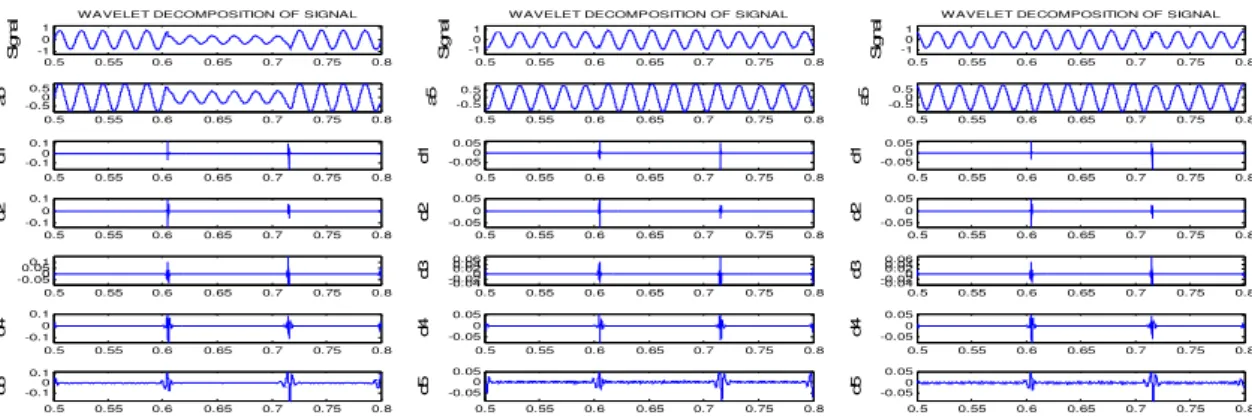
B)

Single line to ground Fault with considering fault resistance i.e R

F

=10

Ω

Here Fault occurs at 9

th

bus on phase A, Fig. 11-18 shows that the fault is in phase A i.e single line to

ground fault, considering fault resistance is equal to 10

Ω

, the voltage at 9

th

bus goes to down but not zero at the

time of fault, when it will occur in case of solidly grounded up to the fault clearing, this indicates that the

importance of fault resistance.

0.5 0.55 0.6 0.65 0.7 0.75 0.8 -1

0 1

S

ignal

0.5 0.55 0.6 0.65 0.7 0.75 0.8 -0.50

0.5

a5

0.5 0.55 0.6 0.65 0.7 0.75 0.8 -0.10

0.1 0.2

d1

0.5 0.55 0.6 0.65 0.7 0.75 0.8 -0.2

-0.10 0.1

d2

0.5 0.55 0.6 0.65 0.7 0.75 0.8 -0.10

0.1

d3

0.5 0.55 0.6 0.65 0.7 0.75 0.8 -0.2

-0.10 0.1

d4

0.5 0.55 0.6 0.65 0.7 0.75 0.8 -0.10

0.1

d5

0.5 0.55 0.6 0.65 0.7 0.75 0.8 -10

1

S

ignal

0.5 0.55 0.6 0.65 0.7 0.75 0.8 -1

0 1

a5

0.5 0.55 0.6 0.65 0.7 0.75 0.8 -0.050

0.05

d1

0.5 0.55 0.6 0.65 0.7 0.75 0.8 -0.050

0.05

d2

0.5 0.55 0.6 0.65 0.7 0.75 0.8 -0.05

0 0.05

d3

0.5 0.55 0.6 0.65 0.7 0.75 0.8 -0.1

-0.050 0.05

d4

0.5 0.55 0.6 0.65 0.7 0.75 0.8 -0.1

-0.050 0.05

d5

0.5 0.55 0.6 0.65 0.7 0.75 0.8 -10

1

S

ignal

0.5 0.55 0.6 0.65 0.7 0.75 0.8 -0.50

0.5

a5

0.5 0.55 0.6 0.65 0.7 0.75 0.8 -0.050

0.05

d1

0.5 0.55 0.6 0.65 0.7 0.75 0.8 -0.050

0.05

d2

0.5 0.55 0.6 0.65 0.7 0.75 0.8 -0.05

0 0.05

d3

0.5 0.55 0.6 0.65 0.7 0.75 0.8 -0.1

-0.050 0.05

d4

0.5 0.55 0.6 0.65 0.7 0.75 0.8 -0.05

0 0.05

d5

Fig. 11. At bus No. 9 fault record from a single-phase to ground of three-phase power System,. are the voltage of phase a, b, and c,

(9)

0.5 0.55 0.6 0.65 0.7 0.75 0.8 -1 0 1

S

ig

nal

0.5 0.55 0.6 0.65 0.7 0.75 0.8 -0.50

0.5

a5

0.5 0.55 0.6 0.65 0.7 0.75 0.8 -50

5 x 10-3

d1

0.5 0.55 0.6 0.65 0.7 0.75 0.8 -505

10 15x 10

-3

d2

0.5 0.55 0.6 0.65 0.7 0.75 0.8 -0.05

0 0.05

d3

0.5 0.55 0.6 0.65 0.7 0.75 0.8 -0.020

0.02

d4

0.5 0.55 0.6 0.65 0.7 0.75 0.8 -0.050

0.050.1

d5

0.5 0.55 0.6 0.65 0.7 0.75 0.8 -1 0 1

S

ig

nal

0.5 0.55 0.6 0.65 0.7 0.75 0.8 -0.50

0.5

a5

0.5 0.55 0.6 0.65 0.7 0.75 0.8 -2

-10 1x 10

-3

d1

0.5 0.55 0.6 0.65 0.7 0.75 0.8 -6

-4 -20

2x 10

-3

d2

0.5 0.55 0.6 0.65 0.7 0.75 0.8 -0.020

0.02

d3

0.5 0.55 0.6 0.65 0.7 0.75 0.8 -20

-100 x 10-3

d4

0.5 0.55 0.6 0.65 0.7 0.75 0.8 -0.04

-0.020 0.02

d5

0.5 0.55 0.6 0.65 0.7 0.75 0.8 -1 0 1

S

ig

nal

0.5 0.55 0.6 0.65 0.7 0.75 0.8 -0.50

0.5

a5

0.5 0.55 0.6 0.65 0.7 0.75 0.8 -50

5 x 10-3

d1

0.5 0.55 0.6 0.65 0.7 0.75 0.8 -50

5 x 10-3

d2

0.5 0.55 0.6 0.65 0.7 0.75 0.8 -0.020

0.02

d3

0.5 0.55 0.6 0.65 0.7 0.75 0.8 -0.010

0.01

d4

0.5 0.55 0.6 0.65 0.7 0.75 0.8 -0.04

-0.020 0.02

d5

Fig. 12. At bus No. 4 fault record from a single-phase to ground of three-phase power System,. are the voltage of phase a, b, and c,

respectively. The fault occurred on phase A at Bus No. 9(Resistance grounding, Rf=10

Ω

)

0.5 0.55 0.6 0.65 0.7 0.75 0.8 -1

0 1

S

ign

al

0.5 0.55 0.6 0.65 0.7 0.75 0.8 -0.50

0.5

a5

0.5 0.55 0.6 0.65 0.7 0.75 0.8 -0.050

0.050.1

d1

0.5 0.55 0.6 0.65 0.7 0.75 0.8 -0.1

0 0.1

d2

0.5 0.55 0.6 0.65 0.7 0.75 0.8 -0.050

0.050.1

d3

0.5 0.55 0.6 0.65 0.7 0.75 0.8 -0.1

0 0.1

d4

0.5 0.55 0.6 0.65 0.7 0.75 0.8 -0.050

0.050.1

d5

0.5 0.55 0.6 0.65 0.7 0.75 0.8 -1

0 1

S

ign

al

0.5 0.55 0.6 0.65 0.7 0.75 0.8 -0.50

0.5

a5

0.5 0.55 0.6 0.65 0.7 0.75 0.8 -0.020

0.02 0.04 0.06

d1

0.5 0.55 0.6 0.65 0.7 0.75 0.8 -0.05

0 0.05

d2

0.5 0.55 0.6 0.65 0.7 0.75 0.8 -0.05

0 0.05

d3

0.5 0.55 0.6 0.65 0.7 0.75 0.8 -0.05

0 0.05

d4

0.5 0.55 0.6 0.65 0.7 0.75 0.8 -0.1

-0.050 0.05

d5

0.5 0.55 0.6 0.65 0.7 0.75 0.8 -1

0 1

S

ign

al

0.5 0.55 0.6 0.65 0.7 0.75 0.8 -0.50

0.5

a5

0.5 0.55 0.6 0.65 0.7 0.75 0.8 -0.020

0.02 0.04 0.06

d1

0.5 0.55 0.6 0.65 0.7 0.75 0.8 -0.05

0 0.05

d2

0.5 0.55 0.6 0.65 0.7 0.75 0.8 -0.020

0.02 0.04

d3

0.5 0.55 0.6 0.65 0.7 0.75 0.8 -0.05

0 0.05

d4

0.5 0.55 0.6 0.65 0.7 0.75 0.8 -0.05

0 0.05

d5

Fig. 13. At bus No. 7 fault record from a single-phase to ground of three-phase power System,. are the voltage of phase a, b, and c,

respectively. The fault occurred on phase A at Bus No. 9 (Resistance grounding, Rf=10

Ω

)

0.5 0.55 0.6 0.65 0.7 0.75 0.8 -1 0 1

S

ig

nal

0.5 0.55 0.6 0.65 0.7 0.75 0.8 -0.50

0.5

a5

0.5 0.55 0.6 0.65 0.7 0.75 0.8 -0.050.050

0.1 0.15

d1

0.5 0.55 0.6 0.65 0.7 0.75 0.8 -0.10

0.1

d2

0.5 0.55 0.6 0.65 0.7 0.75 0.8 -0.1

0 0.1

d3

0.5 0.55 0.6 0.65 0.7 0.75 0.8 -0.2

-0.10 0.1

d4

0.5 0.55 0.6 0.65 0.7 0.75 0.8 -0.10

0.1

d5

0.5 0.55 0.6 0.65 0.7 0.75 0.8 -10

1

S

ig

nal

0.5 0.55 0.6 0.65 0.7 0.75 0.8 -0.50

0.5

a5

0.5 0.55 0.6 0.65 0.7 0.75 0.8 -0.04

-0.020.020 0.04 0.06

d1

0.5 0.55 0.6 0.65 0.7 0.75 0.8 -0.050

0.05

d2

0.5 0.55 0.6 0.65 0.7 0.75 0.8 -0.05

0 0.05

d3

0.5 0.55 0.6 0.65 0.7 0.75 0.8 -0.050

0.05

d4

0.5 0.55 0.6 0.65 0.7 0.75 0.8 -0.1

-0.050 0.05

d5

0.5 0.55 0.6 0.65 0.7 0.75 0.8 -1 0 1

S

ig

nal

0.5 0.55 0.6 0.65 0.7 0.75 0.8 -0.50

0.5

a5

0.5 0.55 0.6 0.65 0.7 0.75 0.8 -0.04

-0.020.020 0.04 0.06

d1

0.5 0.55 0.6 0.65 0.7 0.75 0.8 -0.050

0.05

d2

0.5 0.55 0.6 0.65 0.7 0.75 0.8 -0.04

-0.020.020 0.04 0.06

d3

0.5 0.55 0.6 0.65 0.7 0.75 0.8 -0.050

0.05

d4

0.5 0.55 0.6 0.65 0.7 0.75 0.8 -0.05

0 0.05

d5

Fig. 14. At bus No. 10 fault record from a single-phase to ground of three-phase power System,. are the voltage of phase a, b, and c,

respectively. The fault occurred on phase A at Bus No. 9 (Resistance grounding, Rf=10

Ω

)

0.5 0.55 0.6 0.65 0.7 0.75 0.8 -1

0 1

S

ignal

0.5 0.55 0.6 0.65 0.7 0.75 0.8 -0.50

0.5

a5

0.5 0.55 0.6 0.65 0.7 0.75 0.8 -0.04

-0.020.020.040 0.06 0.08

d1

0.5 0.55 0.6 0.65 0.7 0.75 0.8 -0.050

0.05

d2

0.5 0.55 0.6 0.65 0.7 0.75 0.8 -0.050

0.05

d3

0.5 0.55 0.6 0.65 0.7 0.75 0.8 -0.1

-0.050 0.05

d4

0.5 0.55 0.6 0.65 0.7 0.75 0.8 -0.050

0.05

d5

0.5 0.55 0.6 0.65 0.7 0.75 0.8 -1

0 1

S

ignal

0.5 0.55 0.6 0.65 0.7 0.75 0.8 -0.50

0.5

a5

0.5 0.55 0.6 0.65 0.7 0.75 0.8 -0.020

0.02

d1

0.5 0.55 0.6 0.65 0.7 0.75 0.8 -0.04

-0.020 0.02

d2

0.5 0.55 0.6 0.65 0.7 0.75 0.8 -0.04

-0.020 0.02

d3

0.5 0.55 0.6 0.65 0.7 0.75 0.8 -0.04

-0.020 0.02

d4

0.5 0.55 0.6 0.65 0.7 0.75 0.8 -0.08

-0.06 -0.04 -0.020.020 0.04

d5

0.5 0.55 0.6 0.65 0.7 0.75 0.8 -1

0 1

S

ignal

0.5 0.55 0.6 0.65 0.7 0.75 0.8 -0.50

0.5

a5

0.5 0.55 0.6 0.65 0.7 0.75 0.8 -0.020

0.02

d1

0.5 0.55 0.6 0.65 0.7 0.75 0.8 -0.04

-0.020 0.02

d2

0.5 0.55 0.6 0.65 0.7 0.75 0.8 -0.020

0.02

d3

0.5 0.55 0.6 0.65 0.7 0.75 0.8 -0.04

-0.020 0.02

d4

0.5 0.55 0.6 0.65 0.7 0.75 0.8 -0.04

-0.020 0.02

d5

Fig. 15. At bus No. 11, fault record from a single-phase to ground of three-phase power System,. are the voltage of phase a, b, and c,

(10)

0.5 0.55 0.6 0.65 0.7 0.75 0.8 -1

0 1

S

igna

l

0.5 0.55 0.6 0.65 0.7 0.75 0.8 -0.50

0.5

a5

0.5 0.55 0.6 0.65 0.7 0.75 0.8 -505

10 15x 10

-3

d1

0.5 0.55 0.6 0.65 0.7 0.75 0.8 -0.010

0.01

d2

0.5 0.55 0.6 0.65 0.7 0.75 0.8 -0.05

0 0.05

d3

0.5 0.55 0.6 0.65 0.7 0.75 0.8 -0.020

0.02

d4

0.5 0.55 0.6 0.65 0.7 0.75 0.8 -0.050

0.05

d5

0.5 0.55 0.6 0.65 0.7 0.75 0.8 -1

0 1

S

igna

l

0.5 0.55 0.6 0.65 0.7 0.75 0.8 -0.50

0.5

a5

0.5 0.55 0.6 0.65 0.7 0.75 0.8 -4

-202 4 6x 10

-3

d1

0.5 0.55 0.6 0.65 0.7 0.75 0.8 -50

5x 10

-3

d2

0.5 0.55 0.6 0.65 0.7 0.75 0.8 -0.020

0.02

d3

0.5 0.55 0.6 0.65 0.7 0.75 0.8 -20

-100 x 10-3

d4

0.5 0.55 0.6 0.65 0.7 0.75 0.8 -0.06

-0.04 -0.020 0.02

d5

0.5 0.55 0.6 0.65 0.7 0.75 0.8 -1

0 1

S

igna

l

0.5 0.55 0.6 0.65 0.7 0.75 0.8 -0.50

0.5

a5

0.5 0.55 0.6 0.65 0.7 0.75 0.8 -4

-202 4 6x 10

-3

d1

0.5 0.55 0.6 0.65 0.7 0.75 0.8 -50

5x 10

-3

d2

0.5 0.55 0.6 0.65 0.7 0.75 0.8 -0.020

0.02

d3

0.5 0.55 0.6 0.65 0.7 0.75 0.8 -0.010

0.01

d4

0.5 0.55 0.6 0.65 0.7 0.75 0.8 -0.04

-0.020 0.02

d5

Fig. 16. At bus No. 12, fault record from a single-phase to ground of three-phase power System,. are the voltage of phase a, b, and c,

respectively. The fault occurred on phase A at Bus No. 9 (Resistance grounding, Rf=10

Ω

)

0.5 0.55 0.6 0.65 0.7 0.75 0.8 -1

0 1

Si

g

n

a

l

0.5 0.55 0.6 0.65 0.7 0.75 0.8 -0.50

0.5

a5

0.5 0.55 0.6 0.65 0.7 0.75 0.8 -0.010

0.01 0.02 0.03

d1

0.5 0.55 0.6 0.65 0.7 0.75 0.8 -0.020

0.02

d2

0.5 0.55 0.6 0.65 0.7 0.75 0.8 -0.04

-0.020 0.02 0.04

d3

0.5 0.55 0.6 0.65 0.7 0.75 0.8 -0.020

0.02

d4

0.5 0.55 0.6 0.65 0.7 0.75 0.8 -0.04

-0.020.020.040.060.080

d5

0.5 0.55 0.6 0.65 0.7 0.75 0.8 -1

0 1

Si

g

n

a

l

0.5 0.55 0.6 0.65 0.7 0.75 0.8 -0.50

0.5

a5

0.5 0.55 0.6 0.65 0.7 0.75 0.8 -50

5 10

x 10-3

d1

0.5 0.55 0.6 0.65 0.7 0.75 0.8 -0.01

0 0.01

d2

0.5 0.55 0.6 0.65 0.7 0.75 0.8 -0.020

0.02

d3

0.5 0.55 0.6 0.65 0.7 0.75 0.8 -0.02

-0.010 0.01

d4

0.5 0.55 0.6 0.65 0.7 0.75 0.8 -0.06

-0.04 -0.020.020

d5

0.5 0.55 0.6 0.65 0.7 0.75 0.8 -1

0 1

Si

g

n

a

l

0.5 0.55 0.6 0.65 0.7 0.75 0.8 -0.50

0.5

a5

0.5 0.55 0.6 0.65 0.7 0.75 0.8 -50

5 10

x 10-3

d1

0.5 0.55 0.6 0.65 0.7 0.75 0.8 -0.01

0 0.01

d2

0.5 0.55 0.6 0.65 0.7 0.75 0.8 -0.020

0.02

d3

0.5 0.55 0.6 0.65 0.7 0.75 0.8 -0.010

0.01

d4

0.5 0.55 0.6 0.65 0.7 0.75 0.8 -0.04

-0.020 0.02

d5

Fig. 17. At bus No. 13, fault record from a single-phase to ground of three-phase power System,. are the voltage of phase a, b, and c,

respectively. The fault occurred on phase A at Bus No. 9 (Resistance grounding, Rf=10

Ω

)

0.5 0.55 0.6 0.65 0.7 0.75 0.8 -1

0 1

S

ignal

0.5 0.55 0.6 0.65 0.7 0.75 0.8 -0.50

0.5

a5

0.5 0.55 0.6 0.65 0.7 0.75 0.8 -0.050

0.050.1

d1

0.5 0.55 0.6 0.65 0.7 0.75 0.8 -0.1

0 0.1

d2

0.5 0.55 0.6 0.65 0.7 0.75 0.8 -0.050

0.050.1

d3

0.5 0.55 0.6 0.65 0.7 0.75 0.8 -0.10

0.1

d4

0.5 0.55 0.6 0.65 0.7 0.75 0.8 -0.050

0.050.1

d5

0.5 0.55 0.6 0.65 0.7 0.75 0.8 -10

1

S

ignal

0.5 0.55 0.6 0.65 0.7 0.75 0.8 -0.50

0.5

a5

0.5 0.55 0.6 0.65 0.7 0.75 0.8 -0.020

0.02 0.04

d1

0.5 0.55 0.6 0.65 0.7 0.75 0.8 -0.06

-0.04 -0.020.020 0.04

d2

0.5 0.55 0.6 0.65 0.7 0.75 0.8 -0.04

-0.020 0.02 0.04

d3

0.5 0.55 0.6 0.65 0.7 0.75 0.8 -0.06

-0.04 -0.020.020.040

d4

0.5 0.55 0.6 0.65 0.7 0.75 0.8 -0.05

0 0.05

d5

0.5 0.55 0.6 0.65 0.7 0.75 0.8 -10

1

S

ignal

0.5 0.55 0.6 0.65 0.7 0.75 0.8 -0.50

0.5

a5

0.5 0.55 0.6 0.65 0.7 0.75 0.8 -0.020

0.02 0.04

d1

0.5 0.55 0.6 0.65 0.7 0.75 0.8 -0.06

-0.04 -0.020.020 0.04

d2

0.5 0.55 0.6 0.65 0.7 0.75 0.8 -0.020

0.02 0.04

d3

0.5 0.55 0.6 0.65 0.7 0.75 0.8 -0.06

-0.04 -0.020.020.040

d4

0.5 0.55 0.6 0.65 0.7 0.75 0.8 -0.04

-0.020 0.02 0.04

d5

Fig. 18. At bus No. 14, fault record from a single-phase to ground of three-phase power System,. are the voltage of phase a, b, and c,

respectively. The fault occurred on phase A at Bus No. 9 (Resistance grounding, Rf=10

Ω

)

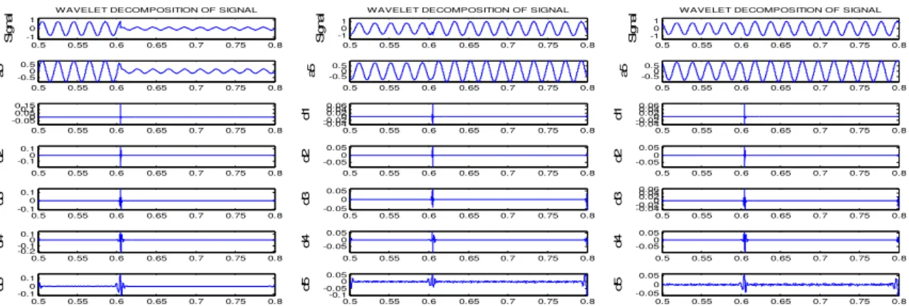
C)

Sudden load applied (50 MW)

Here Sudden load will be applied at 9

th

bus on phase A. Fig. 19-26 clearly shows that the sag appears in

(11)

0.5 0.55 0.6 0.65 0.7 0.75 0.8 -1 0 1

S

ignal

0.5 0.55 0.6 0.65 0.7 0.75 0.8 -0.50

0.5

a5

0.5 0.55 0.6 0.65 0.7 0.75 0.8 -0.1

-0.050 0.05

d1

0.5 0.55 0.6 0.65 0.7 0.75 0.8 -0.1

-0.050 0.05

d2

0.5 0.55 0.6 0.65 0.7 0.75 0.8 -0.05

0 0.05

d3

0.5 0.55 0.6 0.65 0.7 0.75 0.8 -0.04

-0.020 0.02 0.04

d4

0.5 0.55 0.6 0.65 0.7 0.75 0.8 -0.050

0.05

d5

0.5 0.55 0.6 0.65 0.7 0.75 0.8 -1

0 1

S

ignal

0.5 0.55 0.6 0.65 0.7 0.75 0.8 -0.50

0.5

a5

0.5 0.55 0.6 0.65 0.7 0.75 0.8 -0.10

0.1 0.2

d1

0.5 0.55 0.6 0.65 0.7 0.75 0.8 -0.10

0.1

d2

0.5 0.55 0.6 0.65 0.7 0.75 0.8 -0.050

0.050.1

d3

0.5 0.55 0.6 0.65 0.7 0.75 0.8 -0.050

0.05

d4

0.5 0.55 0.6 0.65 0.7 0.75 0.8 -0.050

0.05

d5

0.5 0.55 0.6 0.65 0.7 0.75 0.8 -1

0 1

S

ignal

0.5 0.55 0.6 0.65 0.7 0.75 0.8 -0.50

0.5

a5

0.5 0.55 0.6 0.65 0.7 0.75 0.8 -0.1

-0.050 0.05

d1

0.5 0.55 0.6 0.65 0.7 0.75 0.8 -0.050

0.05

d2

0.5 0.55 0.6 0.65 0.7 0.75 0.8 -0.06

-0.04 -0.020.020 0.04

d3

0.5 0.55 0.6 0.65 0.7 0.75 0.8 -0.020

0.02 0.04

d4

0.5 0.55 0.6 0.65 0.7 0.75 0.8 -0.04

-0.020 0.02

d5

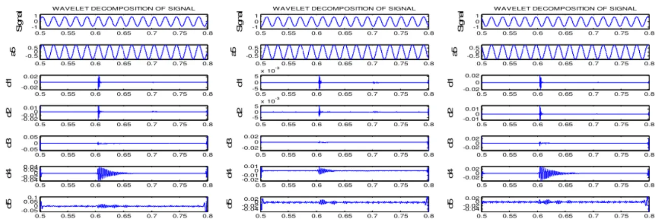
Fig. 19. Voltages of phase a, b, and c, respectively of Bus No. 9. At bus No. 9 sudden load applied of 50 MW.

0.5 0.55 0.6 0.65 0.7 0.75 0.8 -1

0 1

S

ign

al

0.5 0.55 0.6 0.65 0.7 0.75 0.8 -0.50

0.5

a5

0.5 0.55 0.6 0.65 0.7 0.75 0.8 -0.02

0 0.02

d1

0.5 0.55 0.6 0.65 0.7 0.75 0.8 -0.02

-0.010 0.01

d2

0.5 0.55 0.6 0.65 0.7 0.75 0.8 -0.05

0 0.05

d3

0.5 0.55 0.6 0.65 0.7 0.75 0.8 -0.020

0.02

d4

0.5 0.55 0.6 0.65 0.7 0.75 0.8 -0.050

0.050.1

d5

0.5 0.55 0.6 0.65 0.7 0.75 0.8 -10

1

S

ign

al

0.5 0.55 0.6 0.65 0.7 0.75 0.8 -0.50

0.5

a5

0.5 0.55 0.6 0.65 0.7 0.75 0.8 -4

-20 2 4

x 10-3

d1

0.5 0.55 0.6 0.65 0.7 0.75 0.8 -50

5x 10

-3

d2

0.5 0.55 0.6 0.65 0.7 0.75 0.8 -0.02

0 0.02

d3

0.5 0.55 0.6 0.65 0.7 0.75 0.8 -20

-100 x 10-3

d4

0.5 0.55 0.6 0.65 0.7 0.75 0.8 -0.04

-0.020 0.02

d5

0.5 0.55 0.6 0.65 0.7 0.75 0.8 -1

0 1

S

ign

al

0.5 0.55 0.6 0.65 0.7 0.75 0.8 -0.50

0.5

a5

0.5 0.55 0.6 0.65 0.7 0.75 0.8 -2

-10 1

x 10-3

d1

0.5 0.55 0.6 0.65 0.7 0.75 0.8 -8

-6 -4 -202

4x 10

-3

d2

0.5 0.55 0.6 0.65 0.7 0.75 0.8 -0.020

0.02

d3

0.5 0.55 0.6 0.65 0.7 0.75 0.8 -0.010

0.01

d4

0.5 0.55 0.6 0.65 0.7 0.75 0.8 -0.04

-0.020 0.02

d5

Fig. 20. Voltages of phase a, b , and c, respectively of Bus No. 4. At bus No. 9 sudden load applied of 50 MW.

0.5 0.55 0.6 0.65 0.7 0.75 0.8 -1 0 1

S

ign

al

0.5 0.55 0.6 0.65 0.7 0.75 0.8 -0.50

0.5

a5

0.5 0.55 0.6 0.65 0.7 0.75 0.8 -0.04

-0.020.020.040 0.06 0.08

d1

0.5 0.55 0.6 0.65 0.7 0.75 0.8 -0.1

-0.050 0.05

d2

0.5 0.55 0.6 0.65 0.7 0.75 0.8 -0.05

0 0.05

d3

0.5 0.55 0.6 0.65 0.7 0.75 0.8 -0.06

-0.04 -0.020.020 0.04

d4

0.5 0.55 0.6 0.65 0.7 0.75 0.8 -0.050

0.05

d5

0.5 0.55 0.6 0.65 0.7 0.75 0.8 -1 0 1

S

ign

al

0.5 0.55 0.6 0.65 0.7 0.75 0.8 -0.50

0.5

a5

0.5 0.55 0.6 0.65 0.7 0.75 0.8 -0.04

-0.020 0.02

d1

0.5 0.55 0.6 0.65 0.7 0.75 0.8 -0.050

0.05

d2

0.5 0.55 0.6 0.65 0.7 0.75 0.8 -0.020

0.02

d3

0.5 0.55 0.6 0.65 0.7 0.75 0.8 -0.020

0.02 0.04

d4

0.5 0.55 0.6 0.65 0.7 0.75 0.8 -0.06

-0.04 -0.020.020 0.04

d5

0.5 0.55 0.6 0.65 0.7 0.75 0.8 -1 0 1

S

ign

al

0.5 0.55 0.6 0.65 0.7 0.75 0.8 -0.50

0.5

a5

0.5 0.55 0.6 0.65 0.7 0.75 0.8 -0.02

-0.010 0.01

d1

0.5 0.55 0.6 0.65 0.7 0.75 0.8 -0.020

0.02

d2

0.5 0.55 0.6 0.65 0.7 0.75 0.8 -0.010

0.01

d3

0.5 0.55 0.6 0.65 0.7 0.75 0.8 -0.02

0 0.02

d4

0.5 0.55 0.6 0.65 0.7 0.75 0.8 -0.02

-0.010 0.01

d5

Fig. 21. Voltages of phase a, b, and c, respectively of Bus No. 7. At bus No. 9 sudden load applied of 50 MW.

0.5 0.55 0.6 0.65 0.7 0.75 0.8 -1

0 1

S

ign

al

0.5 0.55 0.6 0.65 0.7 0.75 0.8 -0.50

0.5

a5

0.5 0.55 0.6 0.65 0.7 0.75 0.8 -0.050

0.050.1

d1

0.5 0.55 0.6 0.65 0.7 0.75 0.8 -0.2

-0.10 0.1

d2

0.5 0.55 0.6 0.65 0.7 0.75 0.8 -0.050

0.05

d3

0.5 0.55 0.6 0.65 0.7 0.75 0.8 -0.1

-0.050 0.05

d4

0.5 0.55 0.6 0.65 0.7 0.75 0.8 -0.050

0.05

d5

0.5 0.55 0.6 0.65 0.7 0.75 0.8 -1

0 1

S

ign

al

0.5 0.55 0.6 0.65 0.7 0.75 0.8 -0.50

0.5

a5

0.5 0.55 0.6 0.65 0.7 0.75 0.8 -0.050

0.05

d1

0.5 0.55 0.6 0.65 0.7 0.75 0.8 -0.1

0 0.1

d2

0.5 0.55 0.6 0.65 0.7 0.75 0.8 -0.06 -0.04 -0.020 0.02 0.04

d3

0.5 0.55 0.6 0.65 0.7 0.75 0.8 -0.04

-0.020.020 0.04 0.06 0.08

d4

0.5 0.55 0.6 0.65 0.7 0.75 0.8 -0.06 -0.04 -0.020 0.02 0.04

d5

0.5 0.55 0.6 0.65 0.7 0.75 0.8 -1

0 1

S

ign

al

0.5 0.55 0.6 0.65 0.7 0.75 0.8 -0.50

0.5

a5

0.5 0.55 0.6 0.65 0.7 0.75 0.8 -0.04

-0.020 0.02

d1

0.5 0.55 0.6 0.65 0.7 0.75 0.8 -0.04

-0.020.020 0.04 0.06

d2

0.5 0.55 0.6 0.65 0.7 0.75 0.8 -0.02

0 0.02

d3

0.5 0.55 0.6 0.65 0.7 0.75 0.8 -0.020

0.02 0.04

d4

0.5 0.55 0.6 0.65 0.7 0.75 0.8 -0.03

-0.02 -0.010 0.01

d5

(12)

0.5 0.55 0.6 0.65 0.7 0.75 0.8 -1 0 1

S

ig

nal

0.5 0.55 0.6 0.65 0.7 0.75 0.8 -0.50

0.5

a5

0.5 0.55 0.6 0.65 0.7 0.75 0.8 -0.04

-0.020 0.02

d1

0.5 0.55 0.6 0.65 0.7 0.75 0.8 -0.04

-0.020 0.02

d2

0.5 0.55 0.6 0.65 0.7 0.75 0.8 -0.05

0 0.05

d3

0.5 0.55 0.6 0.65 0.7 0.75 0.8 -0.020

0.02

d4

0.5 0.55 0.6 0.65 0.7 0.75 0.8 -0.050

0.050.1

d5

0.5 0.55 0.6 0.65 0.7 0.75 0.8 -1 0 1

S

ig

nal

0.5 0.55 0.6 0.65 0.7 0.75 0.8 -0.50

0.5

a5

0.5 0.55 0.6 0.65 0.7 0.75 0.8 -0.050

0.050.1

d1

0.5 0.55 0.6 0.65 0.7 0.75 0.8 -0.050

0.05

d2

0.5 0.55 0.6 0.65 0.7 0.75 0.8 -0.020

0.02 0.04

d3

0.5 0.55 0.6 0.65 0.7 0.75 0.8 -0.020

0.02

d4

0.5 0.55 0.6 0.65 0.7 0.75 0.8 -0.06

-0.04 -0.020 0.02

d5

0.5 0.55 0.6 0.65 0.7 0.75 0.8 -1 0 1

S

ig

nal

0.5 0.55 0.6 0.65 0.7 0.75 0.8 -0.50

0.5

a5

0.5 0.55 0.6 0.65 0.7 0.75 0.8 -0.04

-0.020 0.02

d1

0.5 0.55 0.6 0.65 0.7 0.75 0.8 -0.020

0.02

d2

0.5 0.55 0.6 0.65 0.7 0.75 0.8 -0.020

0.02

d3

0.5 0.55 0.6 0.65 0.7 0.75 0.8 -0.010

0.01

d4

0.5 0.55 0.6 0.65 0.7 0.75 0.8 -0.020

0.02

d5

Fig. 23. Voltages of phase a, b, and c, respectively of Bus No. 11. At bus No. 9 sudden load applied of 50 MW.

0.5 0.55 0.6 0.65 0.7 0.75 0.8 -10

1

S

igna

l

0.5 0.55 0.6 0.65 0.7 0.75 0.8 -0.50

0.5

a5

0.5 0.55 0.6 0.65 0.7 0.75 0.8 -50

5 10

x 10-3

d1

0.5 0.55 0.6 0.65 0.7 0.75 0.8 -0.010

0.01

d2

0.5 0.55 0.6 0.65 0.7 0.75 0.8 -0.05

0 0.05

d3

0.5 0.55 0.6 0.65 0.7 0.75 0.8 -0.020

0.02

d4

0.5 0.55 0.6 0.65 0.7 0.75 0.8 -0.050

0.050.1

d5

0.5 0.55 0.6 0.65 0.7 0.75 0.8 -1

0 1

S

igna

l

0.5 0.55 0.6 0.65 0.7 0.75 0.8 -0.50

0.5

a5

0.5 0.55 0.6 0.65 0.7 0.75 0.8 -50

5x 10

-3

d1

0.5 0.55 0.6 0.65 0.7 0.75 0.8 -50

5 10

x 10-3

d2

0.5 0.55 0.6 0.65 0.7 0.75 0.8 -0.020

0.02

d3

0.5 0.55 0.6 0.65 0.7 0.75 0.8 -20

-100 x 10-3

d4

0.5 0.55 0.6 0.65 0.7 0.75 0.8 -0.06

-0.04 -0.020 0.02

d5

0.5 0.55 0.6 0.65 0.7 0.75 0.8 -1

0 1

S

igna

l

0.5 0.55 0.6 0.65 0.7 0.75 0.8 -0.50

0.5

a5

0.5 0.55 0.6 0.65 0.7 0.75 0.8 -4

-20 2

x 10-3

d1

0.5 0.55 0.6 0.65 0.7 0.75 0.8 -50

5x 10

-3

d2

0.5 0.55 0.6 0.65 0.7 0.75 0.8 -0.020

0.02

d3

0.5 0.55 0.6 0.65 0.7 0.75 0.8 -0.010

0.01

d4

0.5 0.55 0.6 0.65 0.7 0.75 0.8 -0.04

-0.020 0.02

d5

Fig. 24. Voltages of phase a, b, and c, respectively of Bus No. 12. At bus No. 9 sudden load applied of 50 MW.

0.5 0.55 0.6 0.65 0.7 0.75 0.8 -10

1

S

ign

al

0.5 0.55 0.6 0.65 0.7 0.75 0.8 -0.50

0.5

a5

0.5 0.55 0.6 0.65 0.7 0.75 0.8 -0.010

0.01

d1

0.5 0.55 0.6 0.65 0.7 0.75 0.8 -0.010

0.01

d2

0.5 0.55 0.6 0.65 0.7 0.75 0.8 -0.05

0 0.05

d3

0.5 0.55 0.6 0.65 0.7 0.75 0.8 -0.020

0.02

d4

0.5 0.55 0.6 0.65 0.7 0.75 0.8 -0.050

0.050.1

d5

0.5 0.55 0.6 0.65 0.7 0.75 0.8 -1

0 1

S

ign

al

0.5 0.55 0.6 0.65 0.7 0.75 0.8 -0.50

0.5

a5

0.5 0.55 0.6 0.65 0.7 0.75 0.8 -0.020

0.02

d1

0.5 0.55 0.6 0.65 0.7 0.75 0.8 -0.010

0.01 0.02

d2

0.5 0.55 0.6 0.65 0.7 0.75 0.8 -0.020

0.02

d3

0.5 0.55 0.6 0.65 0.7 0.75 0.8 -0.02

-0.010 0.01

d4

0.5 0.55 0.6 0.65 0.7 0.75 0.8 -0.06

-0.04 -0.020 0.02

d5

0.5 0.55 0.6 0.65 0.7 0.75 0.8 -1

0 1

S

ign

al

0.5 0.55 0.6 0.65 0.7 0.75 0.8 -0.50

0.5

a5

0.5 0.55 0.6 0.65 0.7 0.75 0.8 -0.010

0.01

d1

0.5 0.55 0.6 0.65 0.7 0.75 0.8 -10-5

0 5

x 10-3

d2

0.5 0.55 0.6 0.65 0.7 0.75 0.8 -0.02

0 0.02

d3

0.5 0.55 0.6 0.65 0.7 0.75 0.8 -0.010

0.01

d4

0.5 0.55 0.6 0.65 0.7 0.75 0.8 -0.04

-0.020 0.02

d5

Fig. 25. Voltages of phase a, b, and c, respectively of Bus No. 13. At bus No. 9 sudden load applied of 50 MW.

0.5 0.55 0.6 0.65 0.7 0.75 0.8 -1

0 1

S

ign

al

0.5 0.55 0.6 0.65 0.7 0.75 0.8 -0.50

0.5

a5

0.5 0.55 0.6 0.65 0.7 0.75 0.8 -0.050

0.050.1

d1

0.5 0.55 0.6 0.65 0.7 0.75 0.8 -0.10

0.1

d2

0.5 0.55 0.6 0.65 0.7 0.75 0.8 -0.05

0 0.05

d3

0.5 0.55 0.6 0.65 0.7 0.75 0.8 -0.050

0.05

d4

0.5 0.55 0.6 0.65 0.7 0.75 0.8 -0.050

0.05

d5

0.5 0.55 0.6 0.65 0.7 0.75 0.8 -1

0 1

S

ign

al

0.5 0.55 0.6 0.65 0.7 0.75 0.8 -0.50

0.5

a5

0.5 0.55 0.6 0.65 0.7 0.75 0.8 -0.06

-0.04 -0.020.020.040

d1

0.5 0.55 0.6 0.65 0.7 0.75 0.8 -0.050

0.050.1

d2

0.5 0.55 0.6 0.65 0.7 0.75 0.8 -0.04

-0.020 0.02

d3

0.5 0.55 0.6 0.65 0.7 0.75 0.8 -0.020.020

0.04 0.06

d4

0.5 0.55 0.6 0.65 0.7 0.75 0.8 -0.06 -0.04 -0.020 0.02 0.04

d5

0.5 0.55 0.6 0.65 0.7 0.75 0.8 -1

0 1

S

ign

al

0.5 0.55 0.6 0.65 0.7 0.75 0.8 -0.50

0.5

a5

0.5 0.55 0.6 0.65 0.7 0.75 0.8 -0.02

0 0.02

d1

0.5 0.55 0.6 0.65 0.7 0.75 0.8 -0.020

0.02 0.04

d2

0.5 0.55 0.6 0.65 0.7 0.75 0.8 -0.02

0 0.02

d3

0.5 0.55 0.6 0.65 0.7 0.75 0.8 -0.02

0 0.02

d4

0.5 0.55 0.6 0.65 0.7 0.75 0.8 -0.02

0 0.02