ISSN 0104-6632 Printed in Brazil
Brazilian Journal
of Chemical
Engineering
Vol. 20, No. 04, pp. 445 - 453, October - December 2003
THE MODELLING OF A TEXTILE DYEING
PROCESS UTILIZING THE METHOD
OF VOLUME AVERAGING
A.A.Ulson de Souza
1and S.Whitaker
21
Departamento de Engenharia Química e Engenharia de Alimentos, Universidade Federal de Santa Catarina,
Phone: (+55) (48) 331-9448, Fax: (+55) (48) 331-9687, Cx. P. 476, 88040-900, Florianópolis - SC, Brazil
E-mail: [email protected]
2Department of Chemical Engineering and Material Science,
Phone (+1) (916) 752-8775, Fax (+1) (916) 752-1031 University of California at Davis, CA 95616, U.S.A.
E-mail: [email protected]
(Received: October 25, 2001 ; Accepted: July 3, 2003)
Abstract - In this work the modelling of a process of textile dyeing of a single cotton thread is presented. This thread moves at a constant velocity within a homogeneous dye solution under steady state conditions. The method of volume averaging is applied to obtain the mass transfer equations related to the diffusion and adsorption process inside the cotton thread on a small scale. The one-equation model is developed for the fiber and dye solution system, assuming the principle of local mass equilibrium to be valid. On a large scale, the governing equations for the cotton thread, including the expression for effective diffusivity tensor, are obtained. Solution of these equations permits the dye concentration profile for inside the cotton thread and in the dyeing batch to be obtained and the best conditions for the dyeing process to be chosen.
Keywords: textile, dyeing, modeling.
INTRODUCTION
The problem under study is illustrated in Figure 1, which shows a uniform cotton thread (ω-region), moving at a constant velocity, uo, within a homogeneous
dye solution. The ω-region is composed of fibers (σ -region) and the dye solution inside the thread (β -phase). The concentration of dye in the thread at x = 0 is CAωo, and the concentration in the η-region
at y ~ ∞ is a constant value, CA∞.
A small scale can be identified inside the σ -region as shown in Figure 1. On this small scale, two phases can be characterized: liquid in the microfibers, γ-phase, and solid, κ-phase (Plumb and Whitaker, 1988a, b, 1990). The κ-phase refers to the
cotton microfibers (Trotman, 1975; Holme, 1986), where the adsorption process occurs.
γ - κ SYSTEM AVERAGING
The governing differential equations and boundary conditions for the mass transfer process in both the γ-phase and the κ-phase, illustrated in Figure 1, are given by
(
AA
C
. D C t
γ
)
γ γ
∂ = ∇ ∇
∂ in the γ-phase (1)
As
A C
B.C.1: n .D C
t
γκ γ γ ∂
− ∇ =
A key aspect of the process of spatial smoothing is that the boundary condition given by Eq. (2) is combined with the governing equation. The area average concentration can be replaced by the intrinsic average concentration,
A
A
1
C C
A
γκ γ
γ
γκ
≈
∫
l
Aγ dA
σ
when the
following length-scale constraints, γ << r and
2
r
1 l
σ σ
<<
, are satisfied (Ochoa-Tapia et al.,
1993; Whitaker, 1999).
A
B.C.2 : C γ=f (r, t) at Aγe (3) A
I.C.: C γ=g(r) at t = 0 (4)
It is assumed that in the interface the diffusive flux from the γ-phase to the κ-phase is equal to the adsorption rate.
The κ-phase is assumed to be a rigid phase and the adsorption isotherm is a linear function expressed as
As A
C =KeqC γ at Aγκ (5)
Here CAγ represents the molar concentration of
chemical species under study (mol/m3), CAs
represents the surface concentration (mol/m2), and Dγ is the γ-phase molecular diffusivity of species A (Whitaker, 1992). The entrances and exits of the γ -phase at the boundary of the σ-region are represented by variable Aγe. Variable Aγκis used to represent
the entire interfacial area within that region. The γ -phase and the κ-phase and the σ−β system move at the same velocity in relation to the coordinate system; these two scales are confined to within the cotton fibers.
Here avγκ represents the surface area per unit volume, given by
Aγκ
γκ σ
=
V
av (9)
and the spatial deviation concentration can be expressed as
A A A
C γ=C γ − C γ γ (10) The intrinsic average concentration is defined by
The Closure Problem
A
V
1
C C
V
γ γ
γ γ
=
∫
AγdV (6)At this point a representation for the spatial deviation concentration needs to be developed. The spatial averaging theorem (Howes and
Whitaker, 1985) for volume Vσ can be expressed as
Subtracting Eq. (8) divided by εγ from Eq. (1), one can obtain
A
1
n d
γ γ γκ γ
σ γκ
∇ψ = ∇ ψ +
∫
ψV A (7)
in which Aγκ represents the interfacial area γ-κ contained within averaging volumeVσ .
The integration of Eqs. (1) through (4) in volume
Vσ,using the spatial averaging theorem as presented
by Ochoa-Tapia et al. (1993) and Whitaker (1999), results in the volume-averaged form of Eq. (1), given by
A
A A
A
A A
C t
1
. D C n C dA
C av Keq
t γκ
γ γ γ
γ
γ γ γ
γ γκ
γ
γκ
γ γ γκ
∂
ε =
∂
= ∇ ε ∇ + −
∂ −
∂
∫
V (8)
(
)
A
A
1
A
1
A A
A 1
C
. D C .
t
diffusion accumulation
.D C
diffusive source
D
. n C dA
nonlocal term
C av Keq
t adsorptivesource
γκ
γ
γ γ
γ
− γ
γ γ γ
γ
− γ
γ γκ
σ
γ γ −
γ γκ
∂ = ∇ ∇ ∂
−ε ∇ε ∇ −
−
−ε ∇ +
∂ +ε
∂
∫
V
(11)
A A
A A
C B.C.1: n .D C Keq
t
C
n .D C Keq
t
γ γκ γ γ −
γ γ γ
γκ γ γ
∂ − ∇
∂ ∂
= ∇ +
∂ =
at Aγκ (12)
A
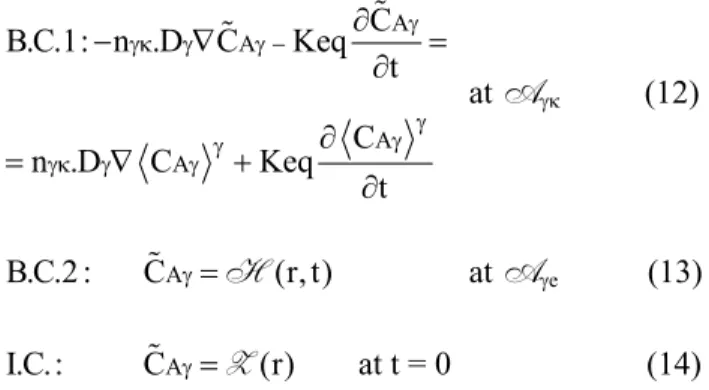
B.C.2 : C γ=H(r, t) at Aγe (13)
A
I.C.: C γ=Z(r) at t = 0 (14)
Since the source H only influences the field over a distance on the order of l
(r, t) CA
A
C
y, we can
generally replace the boundary condition imposed at
Aγe with a spatially periodic condition for
(Whitaker, 1999). So, when the spatially periodic
model is used and
* 2
D t
l
γ γ
is much greater than one,
the boundary value problem can be rewritten as
A A
av Keq C
. C x
D t
γ γ γκ
γ
γ γ
∂ ∇ ∇ = − ε ∂
(15)
A
A
A
B.C.1: n .D C
n .D C
x
C
Keq x
t
γκ γ γ
γ γκ γ γ
γ γ
− ∇ = = ∇
∂ +
∂
+ at Aγκ (16)
A A
B.C.2 : C (rγ + =li) C (r), i 1, 2, 3γ = (17)
Closure Variables where the effective diffusivity tensor is defined by
The boundary value problem for deviation concentration is solved by the method of superposition, where a proposed solution is given by
A
1
D I n bdA
V γκ
γ
γ γκ
∫
+
eff
D = (26)
A
A A C
C b. C
t
γ γ γ
γ= ∇ γ + ∂ + ψ
∂
s (18) and vector u is defined by
A
1
u n D
V
γκ γ
γ γκ
=
∫
s dA (27)Whitaker (1999) proves that ψ = constant is the only solution. Since this additive constant will not pass through the filter, the value of ψ plays no role in the closed form of the volume averaged diffusion equation.
Here the diffusive tensor, Deff, depends only on
the geometry of the porous medium (Whitaker, 1999).
Here b and the scalar s are the closure variables and ψ is an arbitrary function (Whitaker, 1999). The two closure variables can be determined according to the following two boundary value problems:
One can use Eq. (23) and Eq. (27) for estimating the order of s and u. Using these results in Eq. (25), Whitaker (1999) demonstrated that the advective term can be neglected for the case of diffusion in porous solids. The final form of the local average diffusion and transport equation is given by
Problem I
2
b 0
∇ = (19) A
A
av Keq C
1 .
t
γ γ
C γ
γκ γ
γ γ
γ
∂
ε + ε ∂ = ∇ ε ∇
Deff. (28)
B.C.1: − ∇ =n . bγκ nγκ at Aγκ (20)
B.C.2 : b(r+ =li) b(r), i 1, 2, 3= (21)
σ−β SYSTEM AVERAGING
Problem II
In this section we will develop the spatially smoothed equations associated with volume Vω, shown in Figure 1. The length scales related to this averaging volume are identified in Figure 1. The boundary value problem associated with the local volume averaging procedure is given by
2s av Keq
D
γκ γ γ
∇ = − ε
(22)
B.C.1: n . sγκ γ
− ∇ = Keq
D at Aγκ (23)
A
A
av Keq C
1 .
t
γ γ
C γ
γκ γ
γ γ
γ
∂
ε + ε ∂ = ∇ ε ∇
Deff.
B.C.2 : s(r+ =li) s(r), i 1, 2, 3= (24)
(29) Closed Form
in the σ-region
The closed form of the governing equation for the intrinsic average concentration, <CAγ >γ, can be
obtained by substitution of Eq. (18) into Eq. (8). The resulting equation can be expressed as
A
A
B.C.1: n . C
n .D C
γ
σβ γ γ
σβ β β
− ε ∇
− ∇
eff.
D =
at Aσβ (30)
( )
A
A A
av Keq C
1
t
C
. C . u
t
γ γ γκ
γ
γ
γ γ γ
γ
γ γ
∂
ε + ε ∂ =
∂
= ∇ ε ∇ + ∇ ε
∂
eff.
D
(25)
A
B.C.2 : C γ γ =CAβ at Aσβ (31)
A
B.C.3 : C β=G1(r, t) at Aβe (32a)
A
The spatial deviation concentration equation can be obtained by subtracting Eq. (36) divided by ϕσ from Eq. (29), and the resulting equation can be simplified when the following restrictions are satisfied:
r 1 l
ϖ ϖ <<
and
(
l)
1l
ϖ γ σ σ
ε ϕ
>> . Under these
circumstances Eq. (36) can be rewritten as
(
AA
C
. D C
t
β
β
∂ = ∇ ∇
∂ β
)
in the β-phase (33)The σ-Region
Integration of Eq. (29) over V , illustrated in Figure 1, results in
ϖ
av Keq C
1 . t σ γκ σ γ γ γ ∂
ε + ε ∂ = ∇ ε ∇
Deff. C (34)
(
)
1
A
av Keq C
1
t
. . C
n . C dA
σβ σ γκ γ γ σ γ − σ σ σβ γ ϖ ∂
ε + ε ∂ =
= ∇ ε ∇ −
ϕ
−
∫
ε ∇V eff eff D D . (38)
in which the nomenclature for the σ-region has been simplified by using the relationship CAγ γ =Cσ,
where
Cσ = ϕσ Cσ σand
A
B.C.1: n . C
n .D C n . C
σβ γ σ
σ
σβ β β σβ γ
− ε ∇ =
− ∇ + ε ∇
eff.
eff.
D
D σ
at Aσβ (39)
V
1
Cσ Cσ
ϖ σ =
∫
V dV rϖ (35) AB.C.2 : Cσ=C β− Cσ σ at Aσβ (40) By using the averaging theorem and following the
same procedure as that adopted previously and assuming that the restriction l is satisfied, Eq. (34) can be expressed as
σ<< The β-Phase
The volume averaging form of Eq. (33) in volume
Vω, using the averaging theorem, is given by
A
A
av Keq C
1
t
1
. C n C d
1
n . C dA
σβ σβ σ σ γκ σ γ γ σ
σ σ
γ σ σβ
ϖ
σ σβ γ
ϖ
∂
ϕ ε + ε ∂ =
= ∇ ε ϕ ∇ + +
+ ε ∇
∫
∫
. eff. eff D D V VA (36)
A A A A . A A C t accumulation 1
. D C n C dA
V
diffusive transport
1
n D C dA
boundary flux βσ βσ β β β
β
β β βσ β
β
β
βσ β β ω
∂
ϕ ∂ =
= ∇ ϕ ∇ + +
+ ∇
∫
∫
V (41)Here ϕσ represents the volume fraction of the
σ-region contained in the volume Vω .
The Closure Problem
The deviation concentration for the β-phase is given by CAβ = CAβ − CAβ β.
Analogously to the previous procedure, here a representation for the spatial deviation concentration is required. The use of the spatial deviation concentration defined by Gray (1975) and applied to the σ-region results in
The Closure Problem
One can see that the subtraction of Eq. (41) divided by ϕβ from Eq. (33) results in the governing Cσ= Cσ σ+Cσ (37)
One-Equation Model equation for the deviation concentration, which is
given by
Making the assumption that the principle of local mass equilibrium (Quintard and Whitaker, 1993; Whitaker, 1986 a, b) is valid, we can write
(
)
(
)
A
A
1
A A
1
A
1
. A
A
C
. D C
t
diffusive term accumulation
D
. n C dA
nonlocal term
. D C
diffusive source 1
n D C dA
boundary flux βσ
βσ
β
β β
β
− βσ β
β
ω
β
− β β
β β
− βσ β β
β ω
∂ = ∇ ∇ − ∂
−ϕ ∇ −
−ϕ ∇ϕ ∇ −
−ϕ ∇
∫
∫
V
V
(42)
*
A A
C ββ= Cσ σ= C (44)
Here <CΑ>∗ is the spatial average concentration defined as
*
A A
V
A V
1 1
C C dV C
1
C dV
ω σ
β
σ
ω ω
β ω
dV
= = +
+
∫
∫
∫
V
V V
V
(45)
The following definitions
β σ γ
ϕ + ϕ ε = ε (46) By analysis of the order of the terms in Eq. (42), and
assuming the length-scale constraints given by
and lβ << rϖ
*
2
D t
1 l
β β >>
, one can conclude that
the nonlocal term can be considered negligible compared to the diffusion term and the closure process can be considered quasi-steady. Under these circumstances, Eq. (42) can be rewritten as
av Keq K
σ γκ
ϕ = (47)
can be used with Eqs. (36) and (41) to give
(
)
A * *A
C
K . .
t β
∂
ε + = ∇ ϕ ∇
∂ Deff C (48)
(
)
1A .
A
1
. D C n D C dA
βσ
−
β βσ β
β β
ω
∇ ∇ = ϕ
∫
∇V Aβ (43)
Here we have defined the overall effective diffusivity as
(
*)
(
)
*A A
A A
D 1
. . C . D I . C . n C dA n C dA
σβ βσ
β
σ β
β γ σ β β γ σβ β
ω ω
A
σ
∇ ϕ ∇ = ∇ ε ϕ + ϕ ∇ +ε +
Deff Deff
∫
∫
eff
D
V V (49)
Closure Variables The following boundary value problem needs to
be solved: Considering that the local closure problem has a
unique nonhomogeneous term proportional to the gradient of the spatial average concentration evaluated on the centroid, one can write
2b 0
β
∇ = (52)
B.C.1:
(
)
n .D b n . . b
n . D I at A
σβ β β σβ γ σ
σβ β γ σβ
− ∇ = − ε ∇ +
+ − ε
eff
eff
D
D
(53)
*
A A
C β= ∇b .β C + ψ (50)
* A
Cσ=b .σ∇ C + ξ (51)
2b 0
σ
∇ = (55)
Periodicity:
b (r) b (r ) , b (r)
b (r ) , 1, 2,3
σ σ β
β
= +
= + =
li
li i
=
(56)
One can show that ψ = ξ = constant. This constant will not pass through the filter represented by area integrals in Eq. (49), as suggested by Whitaker (1999). So the value of this constant plays no role in the closed-form equation.
The Closed Form
Substituting the expressions given by Eq. (50) and Eq. (51) for the spatial deviation concentrations in Eq. (49), taking into consideration solution of the boundary value problem, one can obtain
(
)
A *(
*)
A
C
K . .
t β
∂
ε + = ∇ ϕ ∇
∂ Deff C (57)
where
(
)
A A
D 1
. n b dA n b
I
σβ βσ
β γ σ β β
β
γ σβ σ βσ
ω ω
ϕ = ε ϕ + ϕ +
+ε f
∫
+∫
eff
ef
D D
D
eff
D
V V β dA
(58)
THE ω -η SYSTEM
The ω-Region
At this point we need to consider the ω-region motion related to the η-phase and for this circumstance the time derivative of average concentration of species A in the ω-region can be expressed as
* *
A A *
A 0 0
d C d C
u . C
u v 0
dt = dt = + ∇ (59)
By simplification Eq. (59), we can write
* *
A A *
A 0 0
d C C
u . C u
dt t
∂
= + ∇
∂ (60)
The subscript on the left side of Eq. (60) does not indicate what is being held constant, but instead
indicates the velocity of the observer who is measuring the concentration. On the basis of Eq. (60) the governing equation for the ω-region can be written as
(
)
(
)
*
A *
A 0
* A
C
K u . C
t
. β . C
∂
ε + + ∇
∂ =
= ∇ ϕ Deff ∇
(61)
The η-Phase
The governing equation for the η-phase is given by
(
A
A
C
. C . D C
t
η
)
A
η η
η η
∂ + ∇ = ∇ ∇
∂ v (62)
One can assume that the boundary layer solution for the hydrodynamic problem in the η-phase is acceptable, and in this circumstance the velocity profiles obtained by Sakiadis (1961a, b, c) can be used in Eq. (62).
CONCLUSIONS
The model of a single cylinder cotton thread, developed using the method of volume averaging for the adsorption dyeing process, represents a fundamental approach in this area. Two scales were considered in order to formulate this problem. The κ -phase, inside the σ-region, is composed of microfibers where the adsorption process occurs. The ω-region, containing the σ-β system, moves at a constant velocity. The method of volume averaging is applied to obtain the mass transfer equations related to the adsorption process on the small and the large scale. The one-equation model is developed for the β- σ system, assuming the local mass equilibrium. The simulation results and validation of this model as well as the effective mass diffusivity obtained by solution of closure problems will be presented in a subsequent paper.
ACKNOWLEGEMENTS
Brazilian Journal of Chemical Engineering,Vol. 20, No. 04, pp. 445 - 453, October - December 2003
Dγ The γ−phase molecular diffusivity, m2/s Aperfeiçoamento de Pessoal de Nível Superior,
CAPES, Brazil. Deff The γ−phase effective diffusivity tensor,
m2/s
Dβ The β−phase molecular diffusivity, m2/s NOMENCLATURE
Dη The η−region molecular diffusivity,
Aγκ Interfacial area of the γ−κ system, m2 m2/s
Deff Effective diffusivity tensor for the σ−β
Aγe Area of entrances and exits for the
γ−phase, m2 system , m2/s
I Unit tensor
Aσβ Interfacial area of the σ−β system, m2
<K> The averaged adsorption equilibrium
Aσe Area of entrances and exits for the
σ−region, m2 constant, Keq Adsorption equilibrium constant, m m
Aβe Area of entrances and exits for the
β−phase, m2 l ω Characteristic length of the ω−region, m
l σ Characteristic length of the σ−region, m Aγκ The γ−κ interfacial area contained
within the averaging volume, Vσ, m2 l β Characteristic length of the β−phase, m
l γ Characteristic length of the γ−phase, m Aγe Area of entrances and exits for the
γ−phase contained within the averaging volume, Vσ, m2
li Lattice vectors describing a spatially
periodic porous medium, m
L Long length for volume averaged Aσβ The σ−β interfacial area contained
within the averaging volume, Vω, m2 quantities associated with the system, m ω−η avγκ The γ−κ interfacial area per unit
volume, m-1 nγκ Outwardly directed unit normal vector pointing from the γ−phase toward the
κ−phase CA∞ Concentration in the η−phase outside
the boundary layer, kgmol/ m3
nσβ Outwardly directed unit normal vector pointing from the σ−region toward the
β−phase CAγ Point concentration in the γ−phase,
kgmol/ m3
<CAγ>γ=Cσ Intrinsic averaged concentration in the
γ−phase, kgmol/ m3 rσ Radius of the γ−κ system averaging volume, Vσ, m
A
C γ Spatial deviation concentration in the
γ−phase, kgmol/ m3
rω Radius of the σ−β system averaging volume, Vω, m
CAβ Point concentration in the β−phase, t Time, s
kgmol/ m3 t* Characteristic time, s
CAη Point concentration in the η−phase, Vσ Small-scale averaging volume, m3
kgmol/ m3 Vω Large-scale averaging volume, m3
<CAβ>β Intrinsic regional averaged uο The ω−region velocity vector, m/s
concentration for the β−phase, kgmol/
m3 vVη The η−phase velocity vector, m/s
γ Volume of the γ−phase contained <Cσ> Superficial regional averaged
concentration for the σ−region, kgmol/ m3
within Vσ, m3
Vσ Volume of the σ−region contained within Vω, m3
<Cσ>σ Intrinsic regional averaged
concentration for the σ−region, kgmol/ m3
δC Mass boundary layer
δH Hydrodynamic boundary layer εγ The γ−phase volume fraction in the Cσ Spatial deviation concentration in the
σ−region, kgmol/ m3 ϕ γ−κ system
σ The σ−region volume fraction in the
A
C β Spatial deviation concentration in the
β−phase, kgmol/ m3
σ−β system
ϕβ The β−phase volume fraction in the <CA>* Intrinsic spatial averaged concentration
for the σ−β system, kgmol/ m3
σ−β system
REFERENCES New York (1993).
Sakiadis, B. C., Boundary-layer Behavior on Continuous Solid Surfaces: I. Boundary-layer Equations for Two-dimensional and Axisymmetric Flow, A.I.Ch.E. Journal, 7, 26-28 (1961a).
Gray, W.G., A Deviation of the Equations for Multiphase Transport, Chemical Engineering Science, 30, 229-233 (1975).
Holme, I., The Effects of Chemical and Physical Properties on Dyeing and Finishing, in C. Preston (ed.), The Dyeing of Cellulosic Fibres, Chap. 3, Dyers’ Company Publications Trust (1986).
Sakiadis, B.C., Boundary-layer Behavior on Continuous Solid Surfaces: II. The Boundary-layer on a Continuous Flat Surface, A.I.Ch.E. Journal, 7, 221-225 (1961b).
Howes, F.A. and Whitaker, S., The Spatial Averaging Theorem Revisited, Chemical Engineering Science, vol. 40, pp. 1387-1392 (1985).
Sakiadis, B.C., Boundary-layer Behavior on Continuous Solid Surfaces: III. The Boundary-layer on a Continuous Cylindrical Surface, A.I.Ch.E. Journal, 7, 467-472 (1961c).
Ochoa-Tapia, Chem. Engng. Sci., c.48 (1993).
Plumb, O.A. and Whitaker, S., Dispersion in Heterogeneous Porous Media I. Local Volume Averaging and Large Scale Averaging, Water Resources Research, 24, 913-926 (1988a).
Trotman E. R., Dyeing and Chemical Technology of Textile Fibres, Charles Griffin & Co. LTD, London (1975).
Whitaker, S., Transient Diffusion Adsorption and Reaction in Porous Catalysts: The Reaction Controlled, Quasi-steady Catalytic Surface, Chemical Engineering Science, 41, 3015-3022 (1986a).
Plumb, O.A. and Whitaker, S., Dispersion in Heterogeneous Porous Media II. Predictions for Stratified and Two-dimensional Spatially Periodic Systems, Water Resources Research, 24,
927-938 (1988b). Whitaker, S., Local Thermal Equilibrium: An
Application to Packed Bed Catalytic Reactor Design, Chemical Engineering Science, 41, 2029-2039 (1986b).
Plumb, O.A. and Whitaker, S., Diffusion, Adsorption and Dispersion in Porous Media: Small-scale Averaging and Local Volume Averaging, in J. H. Cushman (ed.), Dynamics of Fluids in Hierarchical Porous Media, Chap. 5, Academic Press, New York (1990).
Whitaker, S., The Species Mass Jump Condition at a Singular Surface, Chemical Engineering Science, 47, 1677-1685 (1992).
Quintard, M. and Whitaker, S., One and two-equation Models for Transient Diffusion Processes in Two-phase Systems, in Advances in Heat Transfer, 23, 369-465, Academic Press,
Whitaker, S., Theory and Application of Transport in Porous Media: The Method of Volume Averaging, London, Kluwer Academic, 219p (1999).