*e-mail: [email protected]
Feed Forward Neural Network for Prediction of
end Blow Oxygen in LD Converter Steel Making
Narra Rajesha*, Malaya Ranjan Khareb, Shyamal Kumar Pabia
a
Department of Metallurgical and Materials Engineering,
Indian Institute of Technology, Kharagpur, 721302
b
RDCIS- SAIL, Bhilai Steel Plant, Bhilai, 490001
Received: October 23, 2008; Revised: January 14, 2010
A multi layered feed forward neural network model is being developed for the prediction of end blow oxygen in the LD converter using a two step process. In the first step intermediate stopping temperature is being predicted and using this as an input the end blow oxygen is predicted. In both the cases two hidden layers had given the best results compared to the single layer neural network. Intermediate and end blow temperatures played a vital role in end blow oxygen and intermediate stopping temperature predictions. The model acts a guide for the operator and thereby enhances the yield of the converter steel making process.
Keywords: LD converter steel making, feed forward neural networks, end blow oxygen, sensitivity analysis
1. Introduction
LD converter steel making also known as Basic Oxygen Steel making (BOS) or Basic Oxygen Furnace (BOF) process converts hot metal, from blast furnace, and scrap into steel by exothermic oxida-tion of metalloids dissolved in the iron. Oxygen also combines with carbon, eliminating the impurities by gas collection. The main purpose of this process is to decrease carbon percentage from approximately 4.5% to less than 0.08% in liquid steel.
The LD Converter process is a very complex chemical batch process1. The amount and quality of scrap iron change from batch to
batch, the grades of steel produced can change frequently.
A first principles model – called charge balance or static model- which is a complete heat and mass balance of the steel making process is used to predict total oxygen blow necessary to each batch2. However, model mismatches and the unsteady-state nature of
decarburization rate lead to a poor control in end-point temperature and carbon percentage. One procedure to overcome this problem is to take measurements of carbon percentage and temperature during the process and then decarburization rate is determined. Oxygen blown correction is carried out through the ‘end-blow model’3. This model
aims to correlate measurements taken during the process and the end-point conditions of the BOS process. One of the efficient tools, which enable one to obtain a numerical description of this kind of complex process, is the artificial neural networks.
Artificial Neural Networks (ANN), or commonly known as neural networks, have been attractive for applications in complex function modeling and classifications due to the fact that neural networks have very different computing approaches from traditional computing machines4,5. The neural network system has an ability to construct
the rules of input-output mapping by itself. Thus, the designer of the system does not need to know the internal structure and instructions of the system, or the functional rules like traditional systems. Instead, the neural network system requires the feed-in’s of input-output patterns to “learn” before the system can function correctly. Due this flexibility neural networks have gained increasing interest in different fields of material science and other ferrous metallurgical areas6-9.
Several researchers have tried to predict the conditions of the LD converter in the past with varied success10-12. The conditions of
the converter from one plant to the other and from one converter to another in the same plant may vary. Taking these into consideration in this paper, an attempt has been made to predict the end blow oxygen required by using Feed Forward Back Propagation algorithm using the previous heats data of an integrated Steel Plant.
2. Process Description
The integrated steel plant’s steel melting shop (which had chosen for our study) consists of three LD Converters. Each converter pro-duces approximately 120 t of liquid steel from 135 t of charge (Scrap and blast furnace hot metal) in about 45 minutes. Approximately 72 heats are carried out every day.
During the process, hot metal at about 1400°C is converted into steel at 1700 °C by exothermic oxidation of metalloids dissolved in the iron. The converter is a cylindrical steel shell lined with basic refractory materials, such as dolomite and magnesite. The vessel can be rotated 180° on its axis. Oxygen is blown into the vessel with the help of water cooled lance.
manganese and silicon within the melt. Phosphorous is removed by inducing early slag formation by adding powder lime with oxygen. The blow is continued upto a predetermined point (about 88% of the total blow time) and the converter is tilted and temperature is meas-ured by a thermocouple and a sample is taken out for the estimation of carbon. By this time Silicon, Manganese, Phosphorus is almost eliminated. The converter is again kept in vertical position and further blowing is continued. From now onwards oxidation of carbon and iron are predominant. After completion of blowing the converter is tilted and liquid steel is tapped via tap hole and the slag is tapped into the ladles by tilting the converter exactly opposite to the steel tapping side. The time between the sample point and the end of the process is known as the end blow period. The amount of oxygen blown during this period is known as end blow oxygen.
Our aim is to design a model to predict this end blow oxygen so that the desired end point temperature of the steel is reached at the end of the blow without any excessive oxidation of the liquid steel.
3. Design Methodology
For predicting end blow oxygen a two step process is followed. Step I: Predicting the intermediate stopping temperature (Predic-tion model).
Step II: Using this data finding out the required end blow oxygen (Inverse model).
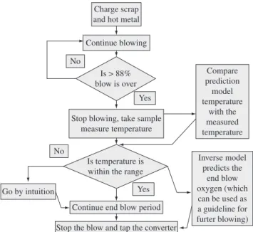
The proposed model’s flow sheet is given in Figure 1.
3.1 Method of analysis
3.1.1. Parameter selection
The selection of process parameters that affect the end blow oxygen is an important step in carrying out the analysis. A survey was conducted in the Integrated Steel Plant’s (ISP) steel melting shop and based on the heuristic knowledge provided by the plant personnel, a total of 6 process parameters viz. Weight of hot metal (tonnes), Weight of scrap (tonnes), End blow oxygen (Nm3), Intermediate
stoppage temperature (°C), Intermediate stoppage Carbon (%), End Blow temperature (°C) are considered. LD converter heat data is taken from the same ISP’s historical data base. Table 1 gives the input and output variables used for the two neural networks.
3.1.2. Data pre-processing
The entire data set contains 1524 records (heat analysis) for a particular converter. In order to design an accurate model the data used is to be distributed evenly and should be in line with the manufacturing process. So certain pre-processing steps are carried out on the raw data and a range has been decided for each parameter. Of 1524 heats 936 heats are remained within the decided range. Table 2 shows the process parameters with their descriptive statistics.
3.1.3. Artificial Neural Network (ANN) modeling
Artificial neural networks are interconnected networks of system of neurons or nodes. A neuron is called a small processing unit which takes input and gives output. A Multi-Layer Perceptron (MLP) is a Feed-Forward neural network having one input layer, one output layer and one or more hidden layers in between them. Each layer is composed of a series of neurons. The output of neurons of one layer becomes input to the neurons of succeeding layer. After selecting the network architecture, the network is trained using learning rate and momentum factor. During the training process the network adjusts its weights to minimize the error between the actual and predicted outputs. The back propagation algorithm13 is
used to adjust the weights. The model is developed using the com-mercial software Statistica14.
The data set is divided in the ratio of 2:1:1 for training, selec-tion and testing respectively. The training data set is used to train the neural network where are all the input variables are fed to the ANN model along with the output variables. The selection data set is used for the selection of the ANN model during training to keep track of over learning of the model14. Test data set is used to
test the developed ANN model for prediction of unknown records. In the test data set input data variables are fed to the developed ANN model without the output variables. Since there are 5 input variables and 1 output variable, the input layer of the network contains 5 neurons and the output layer contains 1 neuron and one hidden layer with 13 neurons. A total of 3 ANN models are trained keeping same values of learning rate and momentum factor6 and number of epochs (iteration) by varying only number
of hidden neurons. The synaptic function is dot product and the output function is sigmoid logistic activation function. The ANN model reports the Root Mean Square Error (RMSE) of the actual and predicted output variables.
Figure1. Proposed model’s flow sheet.
Table 1. Input and output variables for the proposed models.
Prediction model
Inputs Outputs
Weight of hot metal Intermediate stoppage temperature Weight of scrap
End blow oxygen End blow temperature Intermediate stoppage carbon
Inverse model
Inputs Outputs
Weight of hot metal End blow oxygen
Weight of scrap End blow temperature
3.2. Sensitivity analysis
Sensitivity analysis of the developed ANN model with all the process parameters is performed. To check sensitivity of the model with a parameter, that parameter is varied form minimum to maxi-mum including the mean and all other parameters are kept at their corresponding mean levels. The same procedure is repeated for all other process parameters. Then the variation of the end blow oxygen values is observed and the effect of particular parameter is evaluated. This analysis is performed on the best developed network model.
4. Results and Discussion
Descriptive statistics for all input and output variables of the ANN model are shown in Table 2, which includes mean, minimum, maximum and standard deviation.
Three ANN models have been developed separately for both Prediction and Inverse model keeping same learning rate, momentum factor and iteration by only varying the number of neurons in the hidden layers and can be seen in Table 3. The learning rate of 0.05 and momentum Factor of 0.2 are used. The number of iterations for all the topologies is predefined as 5000. All the network models are run for 5000 iterations of back-propagation algorithm during which the inter connecting weights are expected to reach global minimum6.
The error reported is the Root Mean Square Error (RMSE) of the output variable. The training and selection errors first drop sharply
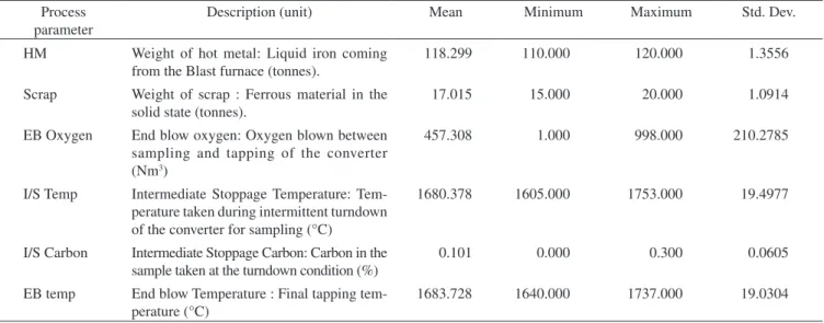
Table 2. Descriptive statistics of the process parameters.
Process parameter
Description (unit) Mean Minimum Maximum Std. Dev.
HM Weight of hot metal: Liquid iron coming from the Blast furnace (tonnes).
118.299 110.000 120.000 1.3556
Scrap Weight of scrap : Ferrous material in the solid state (tonnes).
17.015 15.000 20.000 1.0914
EB Oxygen End blow oxygen: Oxygen blown between sampling and tapping of the converter (Nm3)
457.308 1.000 998.000 210.2785
I/S Temp Intermediate Stoppage Temperature: Tem-perature taken during intermittent turndown of the converter for sampling (°C)
1680.378 1605.000 1753.000 19.4977
I/S Carbon Intermediate Stoppage Carbon: Carbon in the sample taken at the turndown condition (%)
0.101 0.000 0.300 0.0605
EB temp End blow Temperature : Final tapping tem-perature (°C)
1683.728 1640.000 1737.000 19.0304
Table 3. Best three networks.
For prediction model
Network No Network topology Training error Selection error Test error
1 MLP 5-10-6-1 0.049401 0.050971 0.057783
2 MLP 5-25-16-1 0.057511 0.070563 0.069296
3 MLP 5-10-7-1 0.052465 0.057143 0.059974
For Inverse model
Network No Network topology Training error Selection error Test error
1 MLP 5-25-13-1 0.133284 0.134837 0.143504
2 MLP 5-25-19-1 0.134200 0.136889 0.149771
3 MLP 5-25-23-1 0.135179 0.136779 0.147021
Table 4. Error mean and correlation coefficient.
Prediction model Inverse model
Data Mean 1680.378 457.3077
Data S.D 19.487 210.1661
Error Mean 0.160 5.3224
Error S.D 9.695 169.1998
Abs. E mean 4.747 135.9859
S.D Ratio 0.498 0.8051
Correlation 0.867 0.5933
Data Mean is the Average value of the target output variable. Data S.D. is the Standard deviation of the target output variable.
Error Mean is the Average error (residual between target and actual output values) of the output variable.
Abs. E. Mean is the Average absolute error (difference between target and actual output values) of the output variable.
Error S.D. is the Standard deviation of errors for the output variable. S.D. Ratio is the error:data standard deviation ratio.
Correlation is the standard Pearson-R correlation coefficient between the predicted and observed output values.
Table 5. Sensitivity analysis.
Sensitivity analysis for the best Network ( 5-10-6-1) Prediction model
HM Scrap EB temp I/S carbon EB oxygen
Ratio 0.995949 0.996381 1.936454 0.998879 1.348758
Rank 5.000000 4.000000 1.000000 3.000000 2.000000
Sensitivity analysis for the best network ( 5-25-13-1) Inverse model
HM Scrap I/S temp EB temp I/S carbon
Ratio 0.999583 0.996859 1.431237 1.193511 1.034326
Rank 4.000000 5.000000 1.000000 2.000000 3.000000
Figure 2. Prediction model. Figure 3. Inverse model.
Thus the best model is selected where the selection error reaches a minimum value.
The training, selection and test error for all three models along with the best network code is shown in Table 3. It can be observed that the training error for Prediction model network topology 5-10-6-1 is 0.049405-10-6-1 and for Inverse model network topology 5-25-5-10-6-13-5-10-6-1 is 0.133284, which is lower compared to that in the other two topologies. As well the selection error and test error are also lower compared to error in other topologies. The best network topology achieved are 5-10-6-1 (Prediction model) and 5-25-13-1 (Inverse model).
The error mean and correlation coefficient (R) are indicated for the output in Table 4. For a perfect fit of data R = 1. Thus a good network, a high value of R and a low value of mean square error are desirable. Good correlation is achieved for most of the outputs. This suggests that the model is capable of predicting the end blow oxygen effectively.
The observed (actual) versus predicted output values are shown in Figure 2 and 3 for prediction model and inverse models respectively. As can be observed from the figure, most of the predictions are very close to the actual values. However, the predictions are uncertain especially in very low values. The uncertainty can be resulted from the inadequate training for very low values.
Sensitivity analysis indicates which input variables are consid-ered most important by that particular neural network. Sensitivity analysis can be used purely for informative purposes, or to perform input pruning. Sensitivity analysis can give important insights into the usefulness of individual variables. It often identifies variables that can be safely ignored in subsequent analysis, and key variables
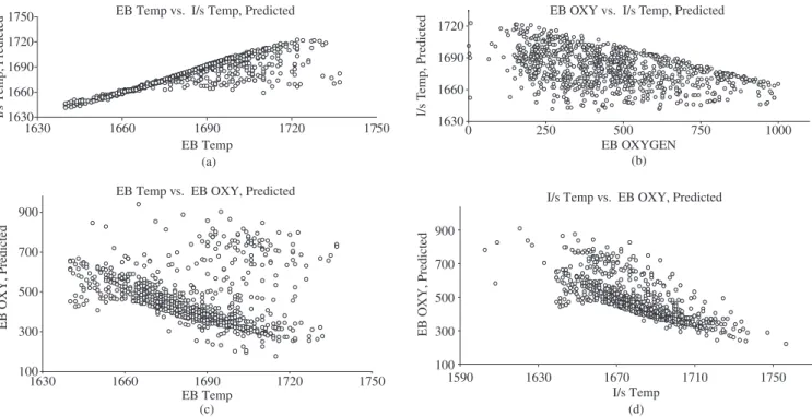
that must always be retained. Sensitivity analysis is performed and is shown in Table 5. The sensitivity graphs of the Prediction model and Inverse model network for the process parameters are shown in Figure 4a-d.
Based on sensitivity analysis the following observations are derived:
• EffectofWeightofHotMetal:Duringthemodeldesignthe
quantity of hot metal is taken as one parameter, but in sensi-tivity analysis it got least importance. So in the models to be considered instead of tonnage its analysis may be taken into the consideration;
• EffectofWeightofScrap:WeightofScrapalsogotthesame
treatment as of hot metal. Scrap as a parameter in tonnage is of less use in modeling;
• EffectofEndBlowTemperature:EndBlowtemperatureof
the previous heats got maximum importance in the prediction model which is used for finding the Intermediate stoppage temperature of the present heat. In case of inverse model which is used for predicting the end blow oxygen it is the second im-portant parameter after intermediate stoppage temperature;
• EffectofIntermediatestoppagetemperature:TheIntermediate
stoppage temperature is having very high impact in predicting the end blow oxygen of the inverse model;
• EffectofIntermediatestoppagecarbon:Asperthesensitivity
Figure 4. a) Sensitivity analysis between EB Temp vs. I/s Temp Predicted; b) Sensitivity analysis between EB OxygenVs I/s Temp Predicted; c) Sensitivity analysis between EB Temp vs. EB Oxygen predicted. and d) Sensitivity analysis between I/s Temp vs. EB Oxygen predicted.
5. Conclusions
Feed forward network using back propagation algorithm is used for the prediction of end blow oxygen in the LD Converter steel making.
5-10-6-1 and 5-25-13-1 architectures with sigmoidal functions are best suited networks for predicting intermediate stopping temperature and end blow oxygen of the LD converter.
Weight of hot metal and Scrap became the secondary parameter while model predictions.
Intermediate stoppage temperature and end blow temperatures stood as the most important parameters in deciding end blow oxygen and intermediate stoppage temperature respectively.
References
1. Turkdogan ET. Fundamentals of Steelmaking. London: The Institute of Materials; 1996.
2. Pehlke RD, Porter WF, Urban RF and Gaines JM. BOF Steelmaking, Introduction, Theory and Design. Warrendale, PA: ISS; 1982. Part I 3. Cox IJ, Lewis RW, Ransing RS, Laszczewski H and Berni G. Application
of neural computing in basic oxygen steel making. Journal of materials processing technology. 2002; 120(3):310-315
4. Haykin S. Neural Networks: A Comprehensive Foundation. 2 ed. Ontario, Canada: McMaster University; 1999.
5. Bishop CM. Neural networks and their applications. Review of scientific instruments. 1994; 65(6):1803-1832.
6. Bhadeshia HKDH. Neural networks in materials science. ISIJ International. 1999; 39(10): 966-979.
7. Hong T, Li J, Bi-qiang Y, Hong-fu L, Jin Y. Evaluation of scheme design of blast furnace based on artificial neural network. Journal of iron and steel research, International. 2008; 15(3):01-05,36
8. Malinov S and Sha W. Application of artificial neural networks for modeling correlations in titanium alloys. Materials science and engineering A. 2004; 365(1):202-211.
9. Radhakrishnan VR and Mohamed AR. Neural networks for the identification and control of blast furnace hot metal quality. Journal of process control. 2000; 10(6):509-524.
10. Kubat C, Taskin H, Artir R and Yilmaz A. Bofy-fuzzy logic control for the basic oxygen furnace (BOF). Robotics and autonomous systems. 2004; 49(3-4):193-205.
11. Horváth G. Neural Networks in Systems Identification. In: Ablameyko S, Goras L, Gori M and Piuri V, editors. Neural Networks in Measurement Systems. IOS Press; 2002. p. 43-78.
12. Feliti AMF, Pacianotto TA and Cunha AP. Neural modeling helps the BOS process to achieve aimed end-point conditions in liquid steel. Engineering Applications of Artificial Intelligence. 2006; 19(1):9-17.
13. Rumelhart DE, Hinton GE and Williams RJ. Learning representations by back-propagating errors. Nature. 323(9):533-536.