processing. This proposition is still applied and accepted by publica-tions of the highest level6-9.
The nonlinear regression method is being used as an alterna-tive way of obtaining the parameters for kinetic crystallization models, such as Nakamura’s10,11, Kamal and Chu’s12, and Dietz13 and Malkin’s14, directly from the non-isothermal crystallization data obtained by DSC. In most cases, the results obtained through this method are considered good. The literature contains reports of unsatisfactory results related to nonlinear regression; however, these unsatisfactory results are more likely to be justified by the limitations of the model of crystallization kinetics in describing the non-isothermal crystallization of the polymer than by the nonlinear regression method itself13,15.
One advantage of nonlinear regression is that it requires less work than the master curve approach. However, in order to perform non-linear regression, which is usually based on the Leven-Marquardt12,13 method, sophisticated software is indispensable. The master curve approach has the advantage that it can be applied through any electronic spreadsheet. These two methods are usually employed after previous correction of the temperature lag between the DSC oven and the polymeric sample; in this aspect, they are both equally work-intensive.
The master curve approach requires the kinetic crystallization model to be in the form of Equation 1[1]. Other equations, such as Malkin’s1,16, also fit this model; however, the method is applied
1. Introduction
Some of the most important industrial polymers are semi-crystalline. This causes them to crystallize during the cooling phase of processing, affecting both properties and processing conditions. Therefore, it is important to incorporate the crystallization phenom-enon in polymer processing simulation programs. However, one of the difficulties in incorporating the crystallization process in com-mercial software is the need for easy, fast and reliable methods for determining the parameters of the kinetic model chosen to describe the crystallization process.
In three previous works of the present authors, the Master Curve Approach proposed by Isayev et al.1 was applied to calculate the non-isothermal crystallization rate constant K(T) for modified polypropylenes2,3 (maleic anhydride and acrylic acid grafted poly-propylenes) and for a heterophasic polypropylene sample (Polypro-pylene/Ethylene-propylene rubber PP/EPR)4,5. The non-isothermal crystallization rate constant obtained by this method was used to calculate the curves of relative crystallinity as a function of tempera-ture at different cooling rates. These simulated curves were highly consistent with the experimental data obtained by DSC. One of the major advantages of the Master Curve Approach is the possibility of using non-isothermal experiments, which allow for the determination of kinetic data at lower temperatures than if only isothermal experi-ments were used. Therefore, these data are more representative of the conditions in which crystallization takes place during polymer
Determination of Non-Isothermal Crystallization Rate
Constant for
Pseudo-Experimental
Calorimetric Data
Viviane Verona Galeraa, Alessandra Lucas Marinellib, Benjamim de Melo Carvalhoa*
a
Department of Materials Engineering, Universidade Estadual de Ponta Grossa – UEPG,
84030-900 Ponta Grossa - PR, Brazil
b
Centro de Caracterização e Desenvolvimento de Materiais – CCDM,
Universidade Federal de São Carlos – UFSCar, 13560-905 São Carlos - SP, Brazil
Received: October 19, 2008; Revised: March 22, 2009
In the present work, non-isothermal crystallization data in the form of heat flow vs. temperature curves were generated using the Nakamura Model and its typical parameters reported in the literature for polypropylene. The values obtained for these curves were added to experimental baselines of a DSC to introduce typical noises in the calorimetric traces generated. The Master Curve Approach was applied by one of the authors to retrieve the non-isothermal crystallization rate constant for these simulated curves without information about the conditions used to generate these pseudo-experimental curves. Thus, the applicability of the Master Curve Approach was tested for data perfectly described by the Nakamura Model. With this procedure, the authors were able to check the sensitivity of the method to uncertainties in the determination of the induction time. The results showed good agreement between the pseudo-experimental curves and the curves simulated using the retrieved non-isothermal crystallization rate constant. However, this good agreement was only possible due to a compensation effect, because some of the parameters showed significant differences between the pseudo-experimental and retrieved values. Among these parameters are the pre-exponential factor of the non-isothermal crystallization rate constant, the temperature of the onset of the crystallization process, and the initial degree of crystallinity of the differential form of the Nakamura Model. These problems were not caused by the Master Curve Approach, but by inherent difficulties in the DSC analysis.
Keywords: Master Curve Approach, non-isothermal crystallization, pseudo-experimental
aT(Tij) is being calculated. So, for a constant degree of crystallinity j at each cooling rate (for example θ = 0.1), the shift factor aT(Tij) relates to the non-isothermal rate constant at the corresponding temperatures at which θ = 0.1 is reached. Trj is the temperature at which θ = 0.1 for the cooling rate taken as reference. For example, if 10 °C/min is chosen as the reference cooling condition, for θ = 0.1 Trj will be equal to T10 °C/min; θ =0.1, and K(Trj) = K(T10 °C/min; θ = 0.1) will be the denomina-tor in Equation 2 for this degree of crystallinity. Obviously, the shift factor aT(Tij) will be equal to one for 10 °C/min, because this is the reference condition. However, each i-th degree of crystallinity will have its own reference temperature Trj, as for example, for θ = 0.5, Trj = T10 °C/min; θ = 0.5. If a temperature Tr is chosen among the Trj temperatures as the overall reference temperature (e.g., Tr = T10 °C/min; θ = 0.1), the plots of aT (Tij) vs. Tij at a constant degree of crystallinity, j, can be shifted to obtain a single plot of the shift factor as a function of temperature, aT (T) vs. T.
From the aT (T) vs. T curve, Isayev et al.1 defined the reduced time for non-isothermal crystallization, ξ, with respect to the refer-ence temperature, Tr, as follows:
ξ = ∫a (T(t’))dtT
t
0
(3)
where
aT( ) ( ) ( )
T K T
K TR
= (4)
The θ vs. ξ curves for the different cooling rates should fall on an isothermal master curve at the general reference temperature Tr. This means that the reduced time transforms the non-isothermal crystallization data into isothermal crystallization data at this refer-ence temperature. Thus, the half-time of crystallization (t1/2)Tr at the reference temperature can be evaluated from the isothermal master curve.
The non-isothermal crystallization rate constant at the reference temperature is therefore obtained from the following equation:
K T t
R
n
Tr
( ) (ln ) ( / )
= 2
1
1 2
(5)
where n is the Avrami index, which is 3 in this case. From K(Tr) and Equation 4, K(T) can be calculated for the whole range of tempera-tures in which the shift factor aT vs. T was calculated. The K(T) vs. T data can then be fitted by the Hoffman & Lauritzen equation18:
K T t U R T T K T Tf n o g
( ) (ln ) exp exp
/ = − − ∞ − 2 1 1
1 2 ∆
(6)
where (1/t1/2)0 is a pre-exponential factor that includes all terms independent of temperature; U is the activation energy for the transport of crystallizing units across the phase boundary; Kg is the nucleation exponent; T∞ = Tg – 30 K is the temperature below which molecular transport ceases; R is the universal gas constant; ∆T T= m0−T is the degree of supercooling, f = 2T / (T + T)m0 is a correction factor accounting for the reduction in the latent heat of
fusion as the temperature is decreased, and Tm0 is the equilibrium melting temperature.
Using the calculated K(T) and assuming n equal to 3, the differ-ential form of the Nakamura equation10, given by Equation 7, can be used to simulate the dθ/dt vs. T curves, which are integrated to obtain almost exclusively to the Nakamura equation, mostly in Isayev’s
various scientific works6-9. In this respect, nonlinear regression is more flexible; moreover, it can be applied to other types of equa-tion, not only to those that fit into the form of Equation 1. Nonlinear regression is being used by different researchers in various research groups11-15. Difficulty in identifying the temperature at the beginning of the crystallization process is inherent to DSC experiments; thus, it occurs in both methods2,17.
In the analysis and manipulation of the data to apply the Master Curve Approach, the present authors2-5, found that one of the main problems was the difficulty in determining the experimental induc-tion time, which is a problem inherent to DSC analysis. It would be very useful to have experimental crystallization data for a polymer sample that: a) is perfectly described by a kinetics model such as the Nakamura equation; b) whose exact non-isothermal rate constant and corresponding induction time are known; and c) whose temperature lag between the DSC furnace and the sample are known exactly. In this case, some kind of validation could be made of the available procedures for calculating the kinetic parameters. Unfortunately, these ideal conditions do not exist.
Therefore, this work presents a methodology that can meet the aforementioned ideal conditions. To this end, pseudo-experimental non-isothermal crystallization curves were generated at different cooling rates using the Nakamura Model10. Thus, for these pseudo-experimental curves, any problem in the Master Curve Approach must be attributed to errors in the process of calculating the kinetic parameters. By using the pseudo-experimental curves, it is possible to know how close the retrieved parameters are from the parameters used to build the pseudo-experimental curves.
To minimize the influence that previous knowledge of the kinetic parameters used to generate the pseudo-experimental curves would have exerted, the author who applied the Master Curve Approach did not receive previous information about the kinetic parameters of the pseudo-experimental data generated by the other author. Thus, a blind analysis was performed. This procedure will be made clearer in the Methodology section.
1.1. Theoretical background
The fundaments of the Master Curve Approach are well described in the paper of Isayev et al.1 and will be mentioned only briefly herein. The Master Curve Approach is based only on experimental crystal-lization data and on the validity of the following general equation to express the crystallization kinetics:
d
dt K T f
θ= θ
( ) ( ) (1)
where θ is the degree of crystallinity, T the temperature and t the time. Equation 1 assumes that the crystallization rate is a product of two functions: K(T), which depends only on temperature, and f(θ), which depends only on the degree of crystallinity. Hence, if there are non-isothermal crystallization data at different cooling rates for a given constant degree of crystallinity in each cooling condition, a shift factor for the non-isothermal crystallization rate constant can be defined according to Equation 2:
d dt d
dt
K T f
K T f
K T K T ij rj ij j rj j ij rj θ θ θ θ
( )
( )
= ( ) ( )= = ( ) ( ) ( )( ) a (TT ijj) (2)
employed to generate the pseudo-experimental calorimetric curves, the original values will be referred to as the “true parameters”.
An additional difficulty was incorporated to the pseudo- experimental data simulated by the Nakamura equation. In this case, the values for the simulated heat flow vs. temperature curves for each cooling rate were added to the respective experimental baseline of a Perkin-Elmer DSC7. Thus, baseline noises caused some imprecision when attributing the temperature corresponding to the beginning of the crystallization process. The pseudo-experimental data represented by heat flow vs. temperature curves were generated by the follow-ing expression:
Q m H d
dt
c
•
= .∆ θ (11)
where Q• and Q m •
are the heat flux in mW and W/g, respectively.
In summary, the following steps were carried out to generate the pseudo-experimental data:
a) Calculation of the induction time tin and the temperature at the onset of crystallization, Tic, for each cooling rate, using Equations 8 and 10, respectively;
b) Calculation of the crystallization rate, dθ/dt, as a function of temperature, using Nakamura equation given by Equation 7, using the parameters reported in the literature;
c) Calculation of the heat flow curve in mW as a function of temperature, based on Equation 11; and
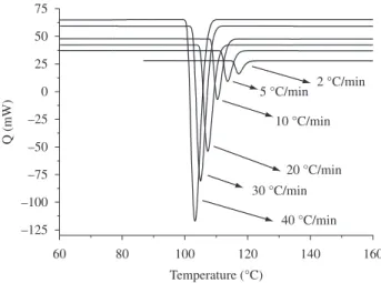
d) Addition of the curve calculated in c to an actual DSC baseline for its respective cooling rate, thereby obtaining the pseudo-experimental curves shown in Figure 1.
Figure 1 shows the pseudo-experimental data after the baseline ad-dition for all the cooling rates used in the present work. These curves correspond to the data sent to the author who applied the Master Curve Approach to retrieve the non-isothermal crystallization rate constant. It is important to point out again that the only information given to this author were the following parameters: U* = 1500 cal/mol; Tg(PP) = –18 °C; Tm° = 172 °C and m = 10 mg. A blind analysis was performed to avoid influencing the results. Thus, the applicability of the method was tested for data described perfectly by the Nakamura Model and parameters known absolutely by only one of the authors. This procedure enabled us to identify exactly what errors could oc-cur in the analysis.
the θ vs. T curves. These simulated data can then be compared with the experimental ones to check the quality of the kinetic parameters calculated by the Master Curve Approach.
d
dt nK T
n n
θ= −θ − −θ −
( )(1 )[ ln(1 )]
1
(7)
1.2. Methodology
As mentioned before, pseudo-experimental calorimetric data were generated by the Nakamura Model, given by Equation 7, using typical parameters reported in the literature. Through this procedure, it is possible to have a very clear idea of how close the retrieved ki-netic parameters calculated by the Master Curve Approach are from the originalvalues. The following parameters for polypropylene19 were used in association with the Nakamura Model to generate the pseudo-experimental data:
U* = 1500 cal/mol;
(Activation energy for molecular transport)
Tg(Polypropylene) = –18 °C; (Glass transition temperature)
Tm° = 172 °C;
(Equilibrium melting temperature)
(1/t1/2)0 = 54,95e7 s–1;
(Pre-exponential factor that includes all terms independent of temperature in the Hoffman & Lauritzen equation)
Kg = 3,99 e5 K2; (Nucleation constant) ∆Hc = –100 J.g–1;
(Latent heat of crystallization ∆Hc)
mass = 10 mg; (Sample mass)
The Nakamura equation does not take into account the induction time for the onset of crystallization. However, this parameter is neces-sary to generate the pseudo-experimental data for applying the Master Curve Approach. This non-isothermal induction time was therefore estimated using the Godovsky and Slonimsky equation20:
t t a
b
in m a
a
= +
+ ( 1)
1 1
(8)
where b is the constant cooling rate; and a and tm are material con-stants independent of temperature.
In a DSC curve, the non-isothermal induction time is calculated by Equation 9:
t T T
b
in= m ic
−
0
(9)
Thus, the initial crystallization temperature that was used in association with the Nakamura equation to generate the pseudo-experimental data was obtained by the following equation:
Tic=Tm0−bt (10)
The following parameters were used to estimate the induction time19: a = 10 and tm = 5.99e18 sK11. From this point forward, when comparing any retrieved kinetic parameters with original values
The author who analyzed the Master Curve Approach saw the pseudo-experimental data as experimental non-isothermal curves obtained for a polymer sample in a DSC. The normal procedure for obtaining the non-isothermal crystallization rate constant was therefore applied using these pseudo-experimental data. Thus, it was necessary to define the temperature of the onset of crystallization (obviously without knowing the true value) for each cooling rate. The θ vs. Temperature curve was thus determined (as well as the corresponding θ vs. time curve for each cooling rate) by applying the method of partial area calculation. Its derivative curve dθ/dt vs. Temperature was thus obtained and the Master Curve Approach was applied to calculate the “unknown” non-isothermal crystallization rate constant that describes the pseudo-experimental data.
2. Results and Discussion
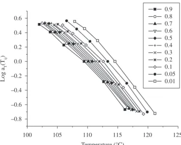
Figure 2 shows the plots of the crystallization rate as a function of sample temperature. As expected, higher cooling rates led to larger and broader peaks and lower onset and peak temperatures, as well as higher crystallization rates. The curves in Figure 2 were used in association with Equation 2 to calculate the aT(Tij) vs. Tij for several constant degrees of crystallinity j, resulting in the curves shown in Figure 3. Thus, the general reference temperature Tr = 111.09 °C was chosen, and the curves of Figure 3 were shifted to obtain the master curve for the shift factor. As can be seen in Figure 4, an excellent superposition of the kinetic data was obtained, even for degrees of crystallinity as low as θ = 0.01 and θ = 0.05. When the Master Curve Approach is applied to experimental data, deviations are usually observed for such low degrees of crystallinity.
Using the shift factor, the reduced time ξ was evaluated for each cooling rate based on Equation 3. Figure 5 shows that a highly defined master curve was obtained for θ vs. time at the reference temperature, Tr =111.09 °C. The parameter (t1/2)Tr was obtained from the master curve θ vs. ξ, and K(TR) was then calculated using Equation 5. Thus, K(T) could be determined as a function of temperature by Equation 4. These values of K(T) were then fitted by Equation 6. In this way, the kinetic parameters (1/t1/2)0 and Kg were retrieved.
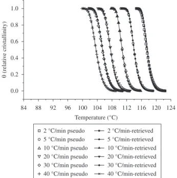
The retrieved non-isothermal crystallization rate constant was used, in association with the Nakamura Model, to build the plots of the relative crystallinity θ as a function of temperature at the various cooling rates. Figure 6 shows an excellent agreement between the pseudo-experimental curves and the simulated curves based on the retrieved parameters. Therefore, it was concluded that the Master
Figure 2. Crystallization rate as a function of sample temperature.
Figure 3. aT(Tij) vs. Tij for several constant degrees of crystallinity j.
Figure 4. Master curve for the shift factor for the non-isothermal crystalliza-tion rate constant as a funccrystalliza-tion of temperature.
Tic value, the crystallization rate predicted by the Nakamura Model in Equation 11 is extremely slow in the initial stages of crystallization. Therefore, the corresponding heat release is insufficient to cause a vis-ible deviation from the baseline. For the author who applied the Master Curve Approach, at the true Tic value in the heat flux vs. temperature curve, there was no evidence that crystallization had begun, so any attempt to attribute a Tic value close to the true temperature would be mere speculation. Therefore, although the retrieved Tic values are not the true ones, they are more plausible because they represent the starting point of a visible deviation from the baselines.
It is now interesting to ascertain if this difference between the true Tic values and the retrieved ones influence the kinetic parameters Kg and (1/t1/2)0 in any way. Table 2 presents a comparison between the true Kg value and (1/t1/2)0 and the corresponding parameters calculated by the Master Curve Approach. This table also compares the retrieved a and tm parameters obtained through the Godovsky and Slonimsky equation using the attributed Tic value and the true ones. As expected, the difference in Tic values leads to differences in the parameters a and tm of the induction time model given by Equation 8.
Table 2 indicates that the calculated Kg is almost identical to the true value. However, the retrieved (1/t1/2)0 is about 4% lower than the true one. Figure 8 shows the non-isothermal rate constant K(T) calculated by Equation 6 for the two sets of parameters. Apparently, the difference between the true K(T) and the retrieved K(T) is not significant. Therefore, it does not explain why the use of different Tic values did not insert errors in the replication of the trueθ vs. T curves, as shown in Figure 6.
To understand the influence of different Tic values and the various parameters of the Nakamura Model on the θ vs. T curves, Figure 9 presents simulated data using a variety of combinations of true and Curve Approach allowed for the determination of the non-isothermal
crystallization rate constant of the Nakamura equation with very high accuracy. It was also concluded that the noises in the baseline did not affect the definition of the induction time (temperature of the onset of crystallization). A third conclusion that should be noted is that the problems in reproducing actual non-isothermal experimental data of polymers by the Nakamura equation using parameters obtained by the Master Curve Approach result from the fact that this model does not provide a perfect description of crystallization kinetics.
If the pseudo-experimental curves in Figure 6 were actual experi-mental data, the analysis would be concluded. It can also be assumed that the kinetic parameters calculated by the Master Curve Approach are very close to the true values because an almost perfect reproduc-tion of the pseudo-experimental data was obtained. However, due to the methodology employed here, this analysis could be taken further to answer the question of how close the retrieved kinetic parameters are from the true values. As mentioned earlier, one of the authors knew the exact true induction times and the true kinetic parameters which were used to build the pseudo-experimental curves. Therefore, it is possible to determine if errors occurred in the blind analysis performed by the other author.
The initial point of the Master Curve Approach is the attribution of the temperature corresponding to the onset of crystallization, Tic, in the DSC curves. Figure 7 shows the Tic values assigned to some cooling rates and the true values initially used to build the pseudo-experimental curves.
As can be seen, the Tic values are approximately 2 °C lower than the true values. Table 1 presents this comparison for all the cooling rates. It also shows the heat of crystallization retrieved from the Master Curve Approach by integrating the partial area between the DSC curve and its baseline. Note that the maximum error obtained in this param-eter is negligible, i.e., about 1% for a cooling rate of 30 °C/min.
The criterion used in attributing values to the temperature corre-sponding to the onset of crystallization is the deviation of DSC trace from its baseline. This deviation corresponds to a minimum heat release that can be detected by the DSC and that can be distinguished from the noises in the baseline. However, Figure 7 indicates that, at the true
Figure 6. Plots of relative crystallinity θ as a function of temperature generated by the Nakamura Model using the true and retrieved (1/t1/2)0 and Kg values.
Figure 7. Attributed Tic values for some cooling rates and true values initially used in the generation of the pseudo-experimental curves.
Table 1. True and retrieved Tic and ∆Hc values.
Cooling rate
True Tic (°C)
Retrieved Tic (°C)
True ∆Hc (J.g–1)
Retrieved ∆Hc (J.g–1)
(2 °C/min) 125.50 122.44 –100 –100.2
(5 °C/min) 121.46 119.17 –100 –100.1
(10 °C/min) 118.18 115.77 –100 –100.1
(20 °C/min) 114.68 112.87 –100 –100.7
(30 °C/min) 112.52 110.9 –100 –101.0
However, because a blind analysis was carried out, the author who applied the Master Curve Approach assumed θt = 0 = 10–3, while the condition used in the generation of the pseudo-experimental data was θt = 0 = 10–14, as proposed by Isayev and Catignani19.
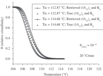
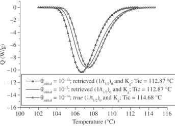
As mentioned earlier, the Nakamura Model presents an extremely slow initial crystallization rate. Thus, in the initial stages of crystal-lization, it takes a considerable amount of time to go from θ = 10–14 to θ = 10–3. To show this significant effect, Figure 10 presents the curves of θ vs. T for these two initial θ, but using only the retrieved set of parameters Tic, (1/t1/2)o and Kg determined by the author who applied the Master Curve Approach. As can be seen, the use of θinitial = 10–3 causes a considerable shift of the θ vs. T curve to higher temperatures compared with the corresponding θ vs. T curve calculated by θinitial = 10–14.
Therefore, the discrepancy between the data in Figures 6 and 9 can be explained based on the fact that, in the former, the retrieved set of parameters Tic, (1/t1/2)0 and Kg were used with θintial equal to 10–3, while in the latter, the true set of parameters was used with θinitial equal to 10–14.
However, in Figure 9 the two sets of parameters were compared using only θinitial equal to 10–14. Thus, the difference in θ
initial compensated for the difference in other parameters, allowing for the excellent con-gruence between the pseudo-experimental data and the retrieved data shown in Figure 6. In Figure 9, due to the use of the same θinitial = 10–14, the difference between the curves obtained by the true and retrieved set of parameters (1/t1/2)0 , Kg and Tic is clearly visible.
Figure 11 presents the heat flow vs. temperature curves gener-ated with different θinitial. Note that there is a significant difference between the true heat flow curve (pseudo-experimental data) and the curve generated using θinitial = 10–14 with the retrieved set of parameters Tic, (1/t1/2)0 and Kg. However, if the retrieved set of pa-rameters is used with θinitial = 10–3, the heat flow curve shifts toward the pseudo-experimental data.
For technological purposes, the description of the crystallization process given by the retrieved values suffices for the simulation of polymer processing. As Figure 6 indicates, the retrieving process allowed for a very good description of the true crystallization kinet-ics. Hence, the crystallinity, the heat release and its influence on the temperature profile would be correctly predicted using this retrieved set of parameters. In this case, the use of θinitial equal to 10–3 is very convenient because it can be used with a Tic that is much easier to define than the true one. As shown in Figure 7, trying to define Tic retrieved parameters for the cooling rate of 20 °C/min. Note that when
the same Tic is used, the crystallization kinetics predicted by the true (1/t1/2)0 and Kg is faster than the one predicted based on the retrieved parameters. This was expected, because true (1/t1/2)0 is 4% higher than the one calculated by the Master Curve Approach. Note, also, that when the same set of parameters (1/t1/2)0 and Kg is used, the θ vs. T curves calculated by the true Tic value are higher than the ones calculated with the retrieved Tic. This was expected, since the Tic value attributed by the author who applied the Master Curve Approach was approximately 2 °C lower than the true one, as shown in Figure 7 and Table 1.
Another comparison that can be made in Figure 9 is between the curves predicted by the true set of parameters (Tic, (1/t1/2)0 and Kg) and the retrieved set of parameters. As can be seen, there is a very significant difference. In this case, the crystallization predicted by the true parameters begins and ends much earlier than that predicted by the retrieved parameters.
However, this latter result seems inconsistent compared with the result presented in Figure 6, which shows an excellent agreement between the pseudo-experimental data and the predicted curves (simulated with the retrieved parameters). After a detailed analysis, it was found that the reason for the difference between Figures 6 and 9 is a peculiarity of the differential form of the Nakamura Model. Equation 7 shows that for θ equal to zero, the rate of crystallization dθ/dt is zero. Therefore, according to the numerical procedure for calculating the progress of the crystallization process, a negligible θt = 0 must be used in Equation 12, albeit different from zero. Otherwise, (dθ/dt)t = 0 will be zero and θt + ∆t will always be zero.
θt t θt θ t
d
dt t
+∆ = + ∆ (12)
Table 2. True and retrieved (1/t1/2)o and Kgvaluesof the non-isothermal crys-tallization rate constant of the Nakamura Model and true and retrieved values of the Godovsky and Sloninsky equation of the induction time.
Parameter True value Retrieved value
(1/t1/2)0 54.95e7 s–1 52.72e7 s–1
Kg 3.990 e5 K2 3.996e5 K2
a 10 11.59
tm 5.99e + 18 sK10 4.99e + 21 s.K11.59
Figure 9. Influence of different Tic values and different (1/t1/2)0 and Kg values of the non-isothermal rate constant on θ vs. T curve for the cooling rate of 20 °C/min.
Figure 8. Non-isothermal rate constant K(T) calculated by Equation 6 for
2. Carvalho BM, Bretas RES. Determinação da constante cinética de cristalização não isotérmica de polipropilenos modificados com ácido acrílico e anidrido maleico. Polímeros 2006; 16(4):305-311.
3. Carvalho BM, Bretas RES. Quiescent crystallization kinetics and morphology of isotatic polypropylene resins of injection molding. III. Non-isothermal crystallization of the heterophasic and graphted polymers.
J Appl Polymer Sci 1999; 72(13): 1741-1753.
4. Marinelli, AL, Carvalho BM, Bretas RES. Evaluation of the master curve approach for the non-isothermal crystallization of PP/EPR. Publicatio UEPG Ciências Exatas e da Terra, Ciências Agrárias e Engenharia 2004; 10(3):13-17.
5. Marinelli AL, Carvalho BM, Bretas RES. Determination of the kinetic crystallization constant for a heterophasic PP using the master curve approach. In: SPE ANTEC Technical Papers. Dallas: Society of Plastics Engineers; 2001. p. 3650-3653.
6. Kim KH, Isayev AI, Kwon K, Sweden CV. Modeling and experimental study of birefringence in injection molding of semicrystalline polymers.
Polymer 2005; 46(12):4183-4203.
7. Kim KH, Isayev AI, Kwon K. Crystallization kinetics for simulation of processing of various polyesters. Journal of Applied Polymer Science
2006; 102(3):2847-2855.
8. Kwon K, Isayev AI, Kim KH. Theoretical and experimental studies of anisotropic shrinkage in injection moldings of various polyesters. Journal of Applied Polymer Science 2006; 102(4):3526-3544.
9. Kim KH, Isayev AI, Kwon K. Flow-induced crystallization in injection molding of polymers: thermodynamic approach. Journal of Applied Polymer Science 2005; 95(3):502-523.
10. Nakamura K, Katayama K, Amano T. Some aspects of nonisothermal crystallization of polymers. II. Consideration of the isokinetic condition.
Journal of Applied Polymer Science 1973; 17(4):1031-1041.
11. Patel RM, Spruiell LJE. Crystallization kinetics during polymer processing: analysis of available approaches for process modeling.
PolymerEngineering and Science 1991; 31(10):730-738.
12. Pérez CJ, Alvarez VA, Stefani PM, Vázquez A. Non-isothermal crystallization of materbi-z/clay nanocomposites. Journal of Thermal Analysis 2007; 88(3)825-832.
13. Alvarez VA, Stefani PM, Vázquez A. Non-isothermal crystallization of polyvinylalcohol-co-ethylene. Journal of Thermal Analysis 2005; 79(1):187-193.
14. Friedl CF, McCafferey NJ. Crystallization prediction in injection molding. In: SPE ANTEC Technical Papers. Montreal: Society of Plastics Engineers; 1991. p. 330-332.
15. Mubarak Y, Harkin-Jones EMA, Martin PJ, Ahmad M. Modeling of non-isothermal crystallization kinetics of isotactic polypropylene. Polymer
2001; 42(7):3171-3182.
16. Ya Malkin A, Beghishev VP, Keapin IA, Bolgov SA. General treatment of polymer crystallization kinetics - Part 1. A new macrokinetic equation and its experimental verification. Polymer Engineering and Science 1984; 24(18):1396-1401.
17. Galera VV, Carvalho BM. Determination of the non isothermal crystallization rate constant of the Nakamura model by non linear regression for using in polymer processing simulation. In: Procedings of Americas Regional Meeting of The Polymer Processing Society. Florianópolis: The Polymer Processing Society/Associaçâo Brasileira de Polímeros; 2004. p.1-2.
18. Hoffman JD, Davis GT, Lauritzen JI. The Rate of Crystallization of Linear Polymers With Chain Folding. In: Hannay NB, editor. Treatise on Solid State Chemistry. New York: Ed. Plenum; 1976. Vol. 3, Chap.7. 19. Isayev AI, Catignani BF. Crystallization and Microstructure in Quenched
Slabs of Various Molecular-Weight Polypropylenes. Polymer Engineering and Science 1997; 37(9):1526-1539.
20. Godovsky YUK, Sloninsky GL. Kinetcs of polymer crystallization from the melt (calorimetric approach). Journal of Polymer Science: Part B: Polymers Physics Edition 1974; 12:1053-1080.
at the true position would be mere speculation, since there is no evidence of any deviation from the baseline.
3. Conclusions
As expected, the Master Curve Approach proved to be completely compatible with non-isothermal crystallization data perfectly described by the Nakamura Model. The imprecision in the determination of the temperature corresponding to the onset of crystallization caused no problems in the description of the pseudo-experimental crystallization data. However, this congruence was possible due to a compensation effect, since there were some differences between the true and retrieved set of parameters (1/t1/2)0 , Tic and θinitial. These problems were not caused by the Master Curve Approach, but by difficulties inherent to the DSC analysis. The use of θinitial equal to 10–3 for the differential form of the Nakamura Model proved to be more convenient than 10–14, because it allowed for the use of a more easily defined Tic.
References
1. Chan TV, Shyu GD, Isayev AI. Master curve approach to polymer crystallization kinetics. Polymer Engineering and Science 1995; 35(9):733-740.
Figure 10. θ vs. T curves for two different initial degrees of crystallinity, but using only the retrieved set of parameters Tic, (1/t1/2)o and Kg.