Comparing CFSR and conventional weather data for discharge and soil loss modelling with SWAT in small catchments in the Ethiopian Highlands

(1)

www.hydrol-earth-syst-sci.net/20/921/2016/ doi:10.5194/hess-20-921-2016

Comparing CFSR and conventional weather data

for discharge and soil loss modelling with SWAT

in small catchments in the Ethiopian Highlands

Vincent Roth1,2,3and Tatenda Lemann1,2,3

1_{Centre for Development and Environment (CDE), University of Bern, Bern, Switzerland} 2_{Sustainable Land Management Research Group, University of Bern, Bern, Switzerland} 3_{Water and Land Resource Centre (WLRC), Addis Abeba, Ethiopia}

Correspondence to:Vincent Roth (vincent.roth@cde.unibe.ch)

Received: 7 August 2015 – Published in Hydrol. Earth Syst. Sci. Discuss.: 27 October 2015 Revised: 6 February 2016 – Accepted: 10 February 2016 – Published: 1 March 2016

Abstract. Accurate rainfall data are the key input parame-ter for modelling river discharge and soil loss. Remote areas of Ethiopia often lack adequate precipitation data and where these data are available, there might be substantial temporal or spatial gaps. To counter this challenge, the Climate Fore-cast System Reanalysis (CFSR) of the National Centers for Environmental Prediction (NCEP) readily provides weather data for any geographic location on earth between 1979 and 2014. This study assesses the applicability of CFSR weather data to three watersheds in the Blue Nile Basin in Ethiopia. To this end, the Soil and Water Assessment Tool (SWAT) was set up to simulate discharge and soil loss, using CFSR and conventional weather data, in three small-scale watersheds ranging from 112 to 477 ha. Calibrated simulation results were compared to observed river discharge and observed soil loss over a period of 32 years. The conventional weather data resulted in very good discharge outputs for all three water-sheds, while the CFSR weather data resulted in unsatisfac-tory discharge outputs for all of the three gauging stations. Soil loss simulation with conventional weather inputs yielded satisfactory outputs for two of three watersheds, while the CFSR weather input resulted in three unsatisfactory results. Overall, the simulations with the conventional data resulted in far better results for discharge and soil loss than simula-tions with CFSR data. The simulasimula-tions with CFSR data were unable to adequately represent the specific regional climate for the three watersheds, performing even worse in climatic areas with two rainy seasons. Hence, CFSR data should not

be used lightly in remote areas with no conventional weather data where no prior analysis is possible.

1 Introduction

(2)

However, the applicability of the CFSR data for small-scale catchments in the Ethiopian Highlands has not been adequately investigated yet. Aforementioned studies did fo-cus on large basins with numerous CFSR stations, which tend to balance errors in rainfall patterns. So far, few stud-ies have been conducted in the Ethiopian context on the im-pact of rainfall data on streamflow simulations. Fuka et al. (2014) used CFSR data in a 1200 km2watershed in Ethiopia with SWAT suggesting CFSR data perform as well or even better than conventional precipitation. Worqlul et al. (2014) correlated conventionally recorded rainfall with CFSR data over the Lake Tana basin (15 000 km2). They suggested that seasonal patterns could adequately be captured although the CFSR data did uniformly overestimate and underestimate measured rainfall. A recent study from Dile and Srinivasan (2014) evaluated the use of CFSR data for hydrological pre-diction using SWAT in the Lake Tana basin, Ethiopia. The study achieved satisfactory results in its simulations for both CFSR and conventional data. While the outcome was bet-ter with conventional weather data, the study concludes that CFSR could be a valuable option in data-scarce regions. Other studies using CFSR data not in the Ethiopian con-text (De Almeida Bressiani et al., 2015; Alemayehu et al., 2015) and with large to very large catchments (13 750 to 73 000 km2) concluded that CFSR data yielded good to very good results and the SWAT model responded reasonably to the data set. One CFSR application in China (Yang et al., 2014) with meso-scale watersheds (366 to 1098 km2) con-cluded that CFSR data were significantly different and that the CFSR data spatial distribution might be the cause for the weak performance.

The impact of spatial variability of precipitation on model run-off showed that standard uniform rainfall assumptions can lead to large uncertainties in run-off estimation (Faurès et al., 2000). Several studies evaluating the CFSR data set have suggested that climatic models tended to overestimate interannual variability but underestimate spatial and seasonal variability (Diro et al., 2009). In another study, Cavazos and Hewitson (2005) performed statistical downscaling of daily CFSR data with Artificial Neural Networks, and their predic-tions showed low performance in near-equatorial and tropical locations, which led them to conclude that the CFSR data are most deficient in locations where convective processes domi-nate. Another study found the CFSR data set performed well on a continental scale but that it failed to adequately repro-duce some regional features (Poccard et al., 2000). A study in China performed streamflow simulations by SWAT using different precipitation sources in a large arid basin using rain gauge data combined with Tropical Rainfall Measuring Mis-sion (TRMM) data (Yu et al., 2011). The study established that streamflow modelling performed better using a combina-tion of TRMM and rain gauge data, as opposed to data from rain gauges only. Different interpolation schemes with the use of univariate and covariate methods showed that

Krig-ing and inverse distance weightKrig-ing performed similarly well when used with the SWAT model (Wagner et al., 2012).

In this paper, WLRC (Water and Land Resource Centre) and SCRP (Soil Conservation Research Programme) rainfall data (hereafter called WLRC data) are compared to CFSR data over a maximum period of 34 years from 1981 to 2014 (Maybar, 33 years for Andit Tid and 32 years for Anjeni). The main objective of this paper is to compare the two data sets for annual, interannual, and seasonal cycles and sub-sequently to compare the effects on discharge and soil loss modelling when using these data sets in three locations in the Ethiopian Highlands (see Fig. 1). Calibrated CFSR modelled discharge and soil loss is then compared to calibrated WLRC modelled discharge and soil loss, and the applicability of the CFSR data in small-scale catchments for hydrological pre-dictions is statistically evaluated and compared.

2 Methods and materials

The effects of spatial and temporal variability in the CFSR rainfall data set for the study area were examined in sev-eral steps. First the CFSR data were statistically compared to measured WLRC rainfall data for accurate representation of annual, interannual, and seasonal cycles. This is important because temporal occurrence of rainfall has a great impact not only on discharge, but moreover on sediment yield gen-eration. Many crop types are sown at the beginning of the rainy season(s), which implies extensive ploughing before-hand, which leaves fields unprotected for the first few rainfall events. Hence, it is clear that temporal occurrences of annual, interannual and seasonal cycles play a crucial role for the val-idation of a data set like the CFSR climatic data. Second, the impact of spatial and temporal variability of rainfall on hy-drology and soil loss was assessed by modelling discharge and soil loss with the SWAT model. The SWAT model was calibrated for discharge once using WLRC climatic data and once using the CFSR climatic data set. Afterwards soil loss was calibrated for each catchment. In a last step, discharge and soil loss on a monthly basis were statistically and visu-ally compared using performance ratings established by Mo-riasi et al. (2007). Each model was calibrated with one to five iterations using 500 simulations each.

2.1 Study area

(3)

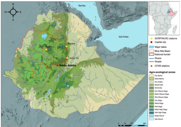
Figure 1.Map overview of Blue Nile (Abbay) Basin with the WLRC research stations, agro-ecological zones according to Hurni (1998), and emplacements of CFSR stations.

with an annual temperature ranging from 12 to 16◦C and a mean annual rainfall ranging from 1211 to 1690 mm. An-jeni has a unimodal rainfall pattern with a main rainy season from June to September, while Andit Tid and Maybar have a bimodal rainfall regime with a small rainy season from April to May (belg) and a main rainy season from June to Septem-ber (kremt) followed by a long dry season from OctoSeptem-ber to March. Land use is dominated by smallholder rain-fed ing systems with grain-oriented production, ox-plough farm-ing, and uncontrolled grazing practises.

2.2 Hydrometeorological data

The hydrometeorological data consist of two sets. The con-ventional or measured data contain daily rainfall and max-imum and minmax-imum temperature from one climatic station for each watershed (Lambrecht Rain Gauge Hellman type with chart recorder, and thermometers). These climatic sta-tions were installed in the early 1980s and span the pe-riod until 2014 with some larger gaps (see Table 1 for de-tails) mainly from 2000 to 2010. The CFSR data (from the Texas A&M University Spatial Sciences website, global-weather.tamu.edu) were obtained for the entire Blue Nile Basin (bounding box: latitude 8.60–12.27◦N and longitude 33.94–40.40◦E) before choosing the four closest stations for each watershed. It includes daily rainfall, maximum and min-imum temperature as well as wind speed, relative humidity,

and solar radiation for 12 locations, 4 for each watershed (see Fig. 1 for details).

2.3 Hydrologic model

(4)

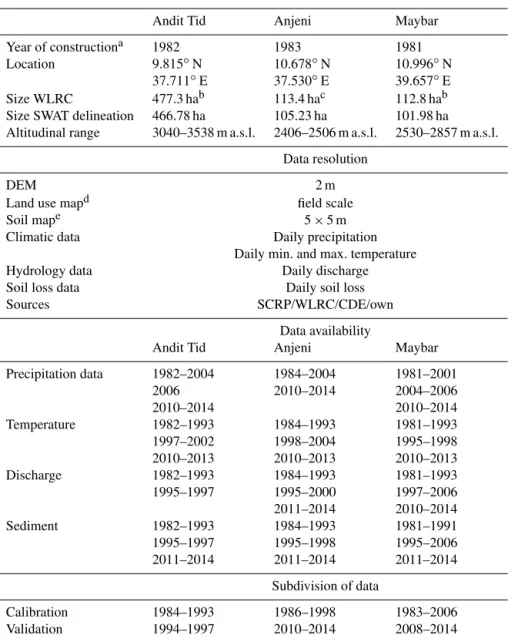
Con-Table 1.Description of study sites, data sources, and time series and gaps. The subdivision of data relates to calibration and validation periods.

Andit Tid Anjeni Maybar

Year of constructiona 1982 1983 1981

Location 9.815◦N 10.678◦N 10.996◦N

37.711◦E 37.530◦E 39.657◦E

Size WLRC 477.3 hab 113.4 hac 112.8 hab

Size SWAT delineation 466.78 ha 105.23 ha 101.98 ha Altitudinal range 3040–3538 m a.s.l. 2406–2506 m a.s.l. 2530–2857 m a.s.l.

Data resolution

DEM 2 m

Land use mapd field scale

Soil mape 5×5 m

Climatic data Daily precipitation

Daily min. and max. temperature

Hydrology data Daily discharge

Soil loss data Daily soil loss

Sources SCRP/WLRC/CDE/own

Data availability

Precipitation data 1982–2004 1984–2004 1981–2001

2006 2010–2014 2004–2006

2010–2014 2010–2014

Temperature 1982–1993 1984–1993 1981–1993

1997–2002 1998–2004 1995–1998

2010–2013 2010–2013 2010–2013

Discharge 1982–1993 1984–1993 1981–1993

1995–1997 1995–2000 1997–2006

2011–2014 2010–2014

Sediment 1982–1993 1984–1993 1981–1991

1995–1997 1995–1998 1995–2006

2011–2014 2011–2014 2011–2014

Subdivision of data

Calibration 1984–1993 1986–1998 1983–2006

Validation 1994–1997 2010–2014 2008–2014

a_{Year of construction is the year the station was built and monitoring started.}b_{Source: Bosshardt (1999).}c_Source:

Bosshardt (1997).dEvery field in the watershed was attributed a land use type on the map.eSource: Belay (2014).

servation Service Curve Number (SCS-CN) method (USDA-SCS, 1972). The flow routing is estimated using the variable storage coefficient method (Williams, 1969) or the Musk-ingum method (Chow, 1959). Soil loss for each HRU is calculated through the Modified Universal Soil Loss Equa-tion. Sediment routing in channels is estimated using stream power (Williams, 1980), and deposition in channels is cal-culated through fall velocity (Arnold et al., 2012; Gassman et al., 2007).

2.4 Spatial data

The spatial data used in ArcSWAT for the present study in-cluded the digital elevation model (DEM), land use data,

(5)

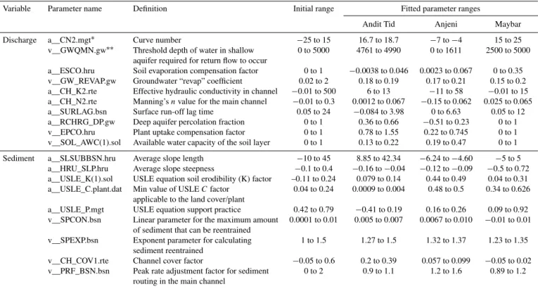
sur-Table 2.SWAT parameters used for discharge and soil loss calibration with initial ranges and fitted final parameter ranges.

Variable Parameter name Definition Initial range Fitted parameter ranges

Discharge a__CN2.mgt∗ _{Curve number} ₋_{25 to 15} _{16.7 to 18.7} ₋_{7 to}₋₄ _{15 to 25}

v__GWQMN.gw∗∗ Threshold depth of water in shallow 0 to 5000 4761 to 4990 0 to 1611 2500 to 5000 aquifer required for return flow to occur

a__ESCO.hru Soil evaporation compensation factor 0 to 1 −0.0038 to 0.046 0.0023 to 0.067 0 to 0.35 v__GW_REVAP.gw Groundwater “revap” coefficient 0.02 to 2 0.18 to 0.19 0.17 to 0.21 0.15 to 0.2 a__CH_K2.rte Effective hydraulic conductivity in channel −0.01 to 500 6 to 13 −11 to 58 −0.01 to 15 a__CH_N2.rte Manning’snvalue for the main channel −0.01 to 0.3 0.0012 to 0.067 −0.15 to 0.062 0.025 to 0.065

a__SURLAG.bsn Surface run-off lag time 0.05 to 24 −0.084 to 3.98 0 to 6.63 0.05 to 12

a__RCHRG_DP.gw Deep aquifer percolation fraction 0 to 1 0.36 to 0.66 −0.51 to 0.23 0 to 1

v__EPCO.hru Plant uptake compensation factor 0 to 1 0.78 to 1.55 0.22 to 0.745 0 to 1

v__SOL_AWC(1).sol Available water capacity of the soil layer 0 to 1 0.13 to 0.22 0.19 to 0.47 0 to 1 Sediment a__SLSUBBSN.hru Average slope length −10 to 45 8.85 to 42.34 −6.24 to−4.60 −5 to 5

a__HRU_SLP.hru Average slope steepness −0.1 to 0.4 −0.16 to−0.04 −0.12 to−0.09 −0.5 to 0.72 a__USLE_K(1).sol USLE equation soil erodibility (K) factor –0.11 to 0.24 0.079 to 0.14 0.44 to 0.49 0.04 to 0.31 a__USLE_C.plant.dat Min value of USLECfactor 0.04 to 0.24 0.0009 to 0.004 0.48 to 0.5 0.34 to 0.626

applicable to the land cover/plant

a__USLE_P.mgt USLE equation support practice 0.42 to 0.79 −0.41 to 0.19 0.16 to 0.26 0.09 to 0.92 v__SPCON.bsn Linear parameter for the maximum amount 0.0001 to 0.01 0.005 to 0.007 0.0067 to 0.010 −0.01 to 0.01

of sediment that can be reentrained

v__SPEXP.bsn Exponent parameter for calculating 1 to 1.5 1.27 to 1.5 1.32 to 1.37 1.23 to 1.35 sediment reentrained

v__CH_COV1.rte Channel cover factor −0.05 to 0.6 0.2 to 0.39 0.057 to 0.099 −0.05 to 0.02 v__PRF_BSN.bsn Peak rate adjustment factor for sediment 0 to 2 0.9 to 1.1 1.2 to 1.6 0.89 to 1.2

routing in the main channel

∗_{a__ means a given value is added to the existing parameter value.}∗∗_{v__ means the existing parameter value is to be replaced by a given value.}

veys carried out by SCRP and WLRC through land use map-ping and interviews and by own surveys in 2008 and 2012. To adapt to annually changing land use patterns, a generic map was adapted from the WLRC land use maps of 2008, 2012, 2014 (Anjeni), and 2010, 2012, 2014 (Andit Tid, Maybar).

2.5 SWAT model setup

The watersheds were delineated using the ArcSWAT delin-eation tool and its stream network compatibility was checked against the stream network from satellite images (one satel-lite image for each watershed). SWAT compiled 1038 HRUs for Anjeni, 1139 HRUs for Maybar, and 728 HRUs for Andit Tid respectively. Using a threshold with this kind of com-bination of small catchments in comcom-bination with highly detailed land use maps would have decreased the avail-able level of information and increased uncertainty for mod-elling. Therefore HRUs were defined using a zero percentage threshold area, which means that all land use, soil, and slope classes were used in the process.

The CFSR time series were complete from 1979 to 2014. The WLRC data had substantial gaps in the time series, mostly in the early 1990s and after 2000 (see Table 1 for de-tails). The SWAT weather generator was used to fill the gaps in the WLRC data set for rainfall and temperature. Otherwise daily precipitation and minimum and maximum temperature data were used to run the model. Potential evapotranspiration was estimated using the Hargreaves method (Hargreaves and

Samani, 1985). Daily river flow and sediment concentration data were measured at the outlet of the three WLRC water-sheds. The flow observations are available throughout the en-tire year, while calculated sediment concentrations from grab samples are only available during rainstorm events and are extrapolated over the whole time period. Personnel at the re-search station are instructed to take grab samples only dur-ing rainfall events, when the river is turndur-ing brown. Grab samples are taken by hand with 1 L bottles which are then filtered through ashless filter papers (retention capacity 12– 25 µm). The filtered sediment samples are later transported to their respective research centres which oven-dry and weight them. Sampling frequency is every 10 min at rising water lev-els and every 30 min after peak water level. The planting and harvesting times were averaged over the entire period and planted at similar dates for the entire simulation. To simulate crop growth, we used the heat unit function in ArcSWAT. Teff (Eragrostis tef), a widely cultivated and highly nutri-tional crop native to Ethiopia, was planted in the beginning of July and harvested in the beginning of December with sev-eral tillage operations preceding planting. Tillage operations were adapted to the usage of the traditional Ethiopian plough called Maresha according to Temesgen et al. (2008), with a tillage depth of 20 cm and a mixing efficiency of 0.3.

(6)

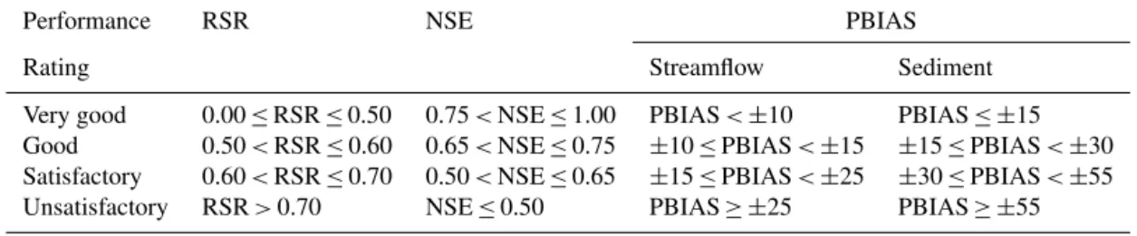
Table 3.General performance ratings recommended by Moriasi et al. (2007).

Performance RSR NSE PBIAS

Rating Streamflow Sediment

Very good 0.00≤RSR≤0.50 0.75<NSE≤1.00 PBIAS<±10 PBIAS≤ ±15 Good 0.50<RSR≤0.60 0.65<NSE≤0.75 ±10≤PBIAS<±15 ±15≤PBIAS<±30 Satisfactory 0.60<RSR≤0.70 0.50<NSE≤0.65 ±15≤PBIAS<±25 ±30≤PBIAS<±55 Unsatisfactory RSR>0.70 NSE≤0.50 PBIAS≥ ±25 PBIAS≥ ±55

validation periods were chosen equally balanced regarding high-flow and low-flow years in all three catchments. The model was first calibrated and validated for discharge and then calibrated and validated for soil loss (see Table 1 for details).

2.6 Calibration setup, validation, and sensitivity analysis

The SUFI-2 algorithm in SWAT-Cup (Abbaspour et al., 2004, 2007) was used for the calibration and validation procedure and for sensitivity, and uncertainty analysis. SWAT-Cup cal-culates the 95 % prediction uncertainty band (95 PPU) in a iterative process. For the goodness of fit, two indices called p factor and r factor are used. Thep factor is the fraction of measured data inside the 95 PPU band, and varies from 0 to 1 where 1 indicates perfect model simulation. Ther fac-tor is the ratio of the average width of the 95 PPU band and the standard deviation of the measured variable. There are different approaches regarding the balance of the p factor andrfactor. Thepfactor should preferably be above 0.7 for discharge and ther factor value should be below 1.5 (Ab-baspour, 2015), but when measured data are of lower quality, other values apply. Once an acceptablepfactor andrfactor are reached, statistical parameters for time series analysis are compared.

For this study we used the Nash–Sutcliffe efficiency (NSE), the Root Mean Square Error-observations standard deviation ratio (RSR), and the percent bias (PBIAS). These are well-known statistical parameters, which are often used for comparison of time series, especially in hydrological modelling (Starks and Moriasi, 2009; Gebremicael et al., 2013; Dile and Srinivasan, 2014; Abbaspour, 2015; De Almeida Bressiani et al., 2015), and therefore help others to compare our modelling results to previous studies. This study refers to the model evaluation techniques described by Mori-asi et al. (2007), who established guidelines for the proposed statistical parameters (see Table 3 for details). The NSE is a normalized statistic that indicates how well a plot of ob-served versus simulated data fits the 1 : 1 line and determines the relative magnitude of the residual variance compared to the measured data variance (Nash and Sutcliffe, 1970). NSE ranges from−∞(negative infinity) to 1, with a perfect con-cordance of modelled to observed data at 1, a balanced

ac-curacy at 0 and a better acac-curacy of observations below zero. The RSR is a standardized root mean square error (RMSE, standard deviation of the model prediction error), which is calculated from the ratio of the RMSE and the standard devi-ation of measured data. RSR incorporates the benefits of er-ror index statistics and includes a scaling factor. RSR varies from the optimal value of 0, which indicates zero RMSE or residual variation, to a large positive value, which indicates a large residual value and therefore worse model simulation performance (Moriasi et al., 2007).

The PBIAS measures the average tendency of the simu-lated values to be larger or smaller than their observed coun-terparts. The optimal value of PBIAS is zero. PBIAS is the deviation of data being evaluated, expressed as a percent-age. A positive PBIAS value indicates the model is under-predicting measured values, whereas negative values indicate over-predicting.

For this article, the recommendations for reported values were strictly applied for discharge calibration and lowered for soil loss calibration.

The model performance was also evaluated using the hy-drograph visual technique, which allows a visual model eval-uation overview to be made. As suggested by Legates and McCabe (1999) this should typically be one of the first steps in model evaluation. Adequate visual agreement between ob-served and simulated data was compared on discharge and soil loss plots on a monthly basis.

3 Results and discussion

3.1 General comparison of CFSR and WLRC rainfall data

(7)

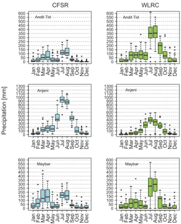
show a main rainy season from July to September and a light rainy season from March to May, while the CFSR data only show mildly increased rainfall in March, April, July, and Au-gust but no distinct rainy season (see Fig. 2 for comparison). The CFSR data for Anjeni highly overestimated rainfall in the region. While WLRC data showed a clear trend towards only one main rainy season from May/June to September with average monthly rainfall ranging from 100 mm (May) to 380 mm (July), the CFSR data showed a pronounced main rainy season with monthly averages ranging from 400 to 1000 mm from June to September and a distinct small rainy season from March to May with monthly averages 3 times as high as the WLRC rainfall data. The total annual CFSR rainfall was 3 times the WLRC annual rainfall.

WLRC Maybar data showed a clear seasonality, with two rainy seasons, one in March and April, and one from July to August. The belg rainy season showed only mild increase of average rainfall to around 75 mm month−1_{and the kremt}

rainy season showed a distinct increase of rainfall to an av-erage of 270 mm month−1. From the CFSR rainfall data, no clear distinction could be made between the belg and the kremt rainy season – both showed a rainfall increase to around 150 mm month−1 and the total annual rainfall was strongly underestimated.

In general, all CFSR rainfall patterns showed a similar composition; data variability was more uniformly distributed and the distinct seasonality of the WLRC data were not well represented. CFSR data underestimated the bimodal rainfall climates and strongly overestimated the unimodal rainfall cli-mate. The WLRC data have a highly variable rainfall range in the bimodal rainfall locations, which is not reflected by the CFSR data. In general, the CFSR rainfall data do not repre-sent the high variability of rainfall measured by WLRC data.

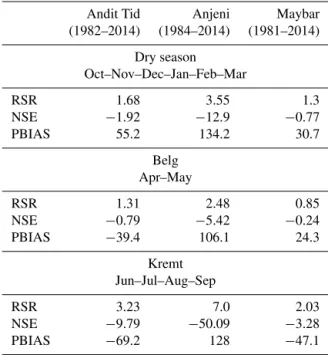
3.1.1 Seasonal comparison of rainfall data

The seasonal components of the CFSR rainfall were as-sessed for the three stations by breaking the monthly data into seasons (dry season from October to March, small rainy season (belg) from April to May, and large rainy season (kremt) from June to September) and by comparing these only. The comparison of measured rainfall to modelled rain-fall for the dry season from October to March was unsatis-factory (NSE<0.50) with negative NSEs for three stations (AT:−1.92, AJ:−12.19, MA:−0.77). The PBIAS indicated model underestimation for Anjeni and Maybar (AJ: 134.2, MA: 30.7) and an overestimation of the rainfall for An-dit Tid (AT: –55.2). The RSR showed large positive values (AT: 1.68, AJ: 3.55, MA: 1.3), indicating a low model sim-ulation performance and again an unsatisfactory rating (see table).

For the belg rainy season from April to May, the model performed badly. Surprisingly, the model performed worst in Anjeni, where no small rainy season occurs. The CFSR model performance for Anjeni was unsatisfactory, with an

Precipitation distribution (1979-2014)

Figure 2.Monthly CFSR and WLRC rainfall distribution of all

sta-tion as box plots with monthly rainfall distribusta-tion. CFSR data from 1979 to 2014 and WLRC data from 1981/1982/1984 to 2014 are shown. See Table 1 for details.

NSE of−5.42, a PBIAS of 106.1, and an RSR of 2.48. The CFSR model overestimated the monthly rainfall in all but 5 out of 22 years. Andit Tid and Maybar were slightly more adequate but still unsatisfactory. NSE was−0.79 and−0.24 respectively, indicating unsatisfactory performance. PBIAS was−39.4 and 24.3, respectively. RSR was 1.31 and 0.85, which again indicates an unsatisfactory result.

The kremt rainy season from June to September is the sea-son with the heaviest rainfall throughout the year. On average some 77 % of the yearly rain falls within this time period. This is also the time period where the heaviest soil erosion occurs induced by rainfall. For Anjeni, Andit Tid, and May-bar, the CFSR model performed unsatisfactorily (see Table 4) with NSEs below 0.50 (AT:−9.79, AJ:−50.09, MA:−3.28), RSRs above 0.70 (AT: 3.23, AJ: 7.0, MA: 2.03), and PBIAS values ranging from−69.2 (AT) and−47.1 (MA) to+128 (AJ).

(8)

Table 4.Seasonal comparison of rainfall time series of daily rainfall amounts. Satisfactory performance ratings are highlighted in bold. Details for duration and gaps can be found in Table 1.

(1982–2014) (1984–2014) (1981–2014)

Dry season Oct–Nov–Dec–Jan–Feb–Mar

RSR 1.68 3.55 1.3

NSE −1.92 −12.9 −0.77

PBIAS 55.2 134.2 30.7

Belg Apr–May

RSR 1.31 2.48 0.85

NSE −0.79 −5.42 −0.24

PBIAS −39.4 106.1 24.3

Kremt Jun–Jul–Aug–Sep

RSR 3.23 7.0 2.03

NSE −9.79 −50.09 −3.28

PBIAS −69.2 128 −47.1

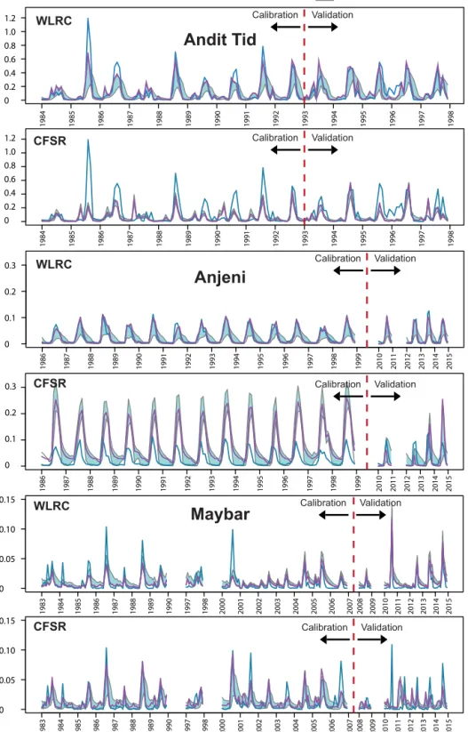
3.2 Discharge modelling with WLRC and CFSR data The performance ratings for each of the three catchments in-cluding SWAT-Cuppfactor andrfactor are summarized in Table 5. The table is divided into discharge comparison and soil loss comparison. Final parameter ranges are presented in Table 2.

3.2.1 Andit Tid

Calibration of Andit Tid with WLRC rainfall data yielded

very good results. With a p factor of 0.71 and an r factor

of 0.53 (see Sect. 2.6 for performance rating) the statistical parameters RSR, NSE, and PBIAS yielded very good results (0.46, 0.79, 3.1 respectively). The CFSR rainfall data, which underestimated the WLRC rainfall pattern, yielded

unsatis-factory results with RSR, NSE, and PBIAS of 0.80, 0.36,

and 31.4. The hydrograph shows that the underestimation of rainfall amounts for Andit Tid did result in a constant under-estimation of peak flows and of base flows throughout the whole time period.

Validation of discharge for Andit Tid with WRLC data showed very good results with RSR: 0.46, NSE: 0.79, and PBIAS 9.6 and marginally unsatisfactory results for the CFSR data set (RSR: 0.74, NSE: 0.45, PBIAS: 37.9).

3.2.2 Anjeni

Anjeni showed very good results for calibration with WLRC rainfall data. RSR, NSE, and PBIAS were well inside the

op-timal performance ratings (0.39, 0.85, and 3.7 respectively); see Table 3 and Fig. 3 for comparison.

Satisfactory calibration could not be reached with CFSR data and neither baseflow, nor peaks could be adequately rep-resented. With ap factor of 0.49 and an r factor of 1.91 the statistical parameters were unsatisfactory (RSR: 2.70, NSE:−6.27, and PBIAS:−226.0). The hydrograph (Fig. 3) shows that the strong overestimation of CFSR rainfall data during belg led to a modelled discharge with extreme peaks during kremt, which do not correspond to the discharge regime of measured WLRC data.

Validation of discharge for Anjeni with WRLC data showed very good results with RSR: 0.41, NSE: 0.83, and PBIAS−6.7 and unsatisfactory results for the CFSR data set with RSR: 1.24, NSE:−0.53, and very good PBIAS: 8.1.

3.2.3 Maybar

Calibration of Maybar with WLRC rainfall data proved to be less straightforward than Anjeni and Andit Tid. The rugged topography of Maybar combined with a inadequate cross section proved challenging to model. Nonetheless, satisfac-toryresults were achieved for discharge with RSR, NSE, and PBIAS of 0.63, 0.60, and−23.4 respectively.

The CFSR rainfall data yielded an unsatisfactory discharge simulation result with RSR, NSE, and PBIAS. As the CFSR-modelled rainfall shows two similar rainy seasons where WLRC rainfall data have distinct belg and kremt rainy sea-sons, SWAT modelled discharge showed similar trends. Fig-ure 3 shows regular discharge peaks from February to March, in accordance to rainfall pattern deviation as seen in Fig. 2, when no increase of discharge was measured at the research station. The SWAT model reflected input rainfall pattern ade-quately, which led to discharge peaks during belg, when there are none in the measured data. At the same time it leads to reduced discharge peaks during kremt, when the measured WLRC data are clearly pronounced.

Validation of discharge for Maybar with WRLC data showed good results with RSR: 0.56, NSE: 0.74, and PBIAS 17.3 and unsatisfactory results for the CFSR data set with RSR: 0.98, NSE: 0.04, and very good PBIAS:−1.9.

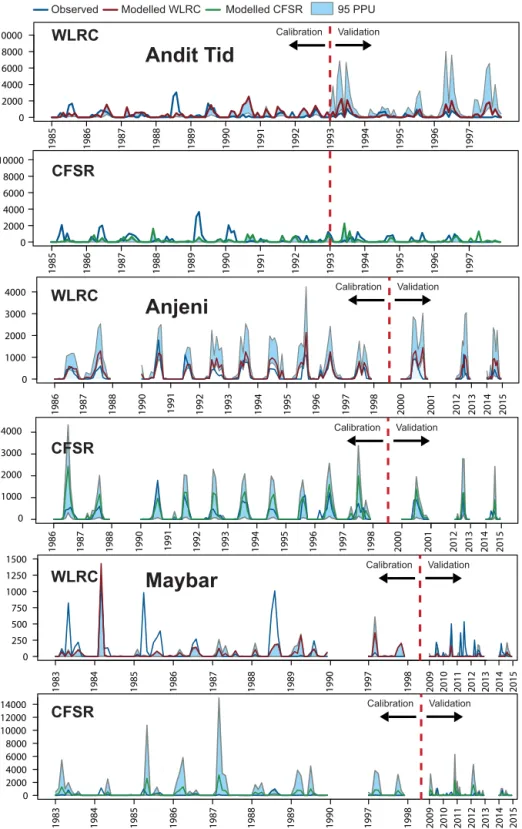
3.3 Soil loss modelling with WLRC and CFSR data

(9)

be-1984 1985 1986 1987 1988 1989 1990 1991 1992 1993 1994 1995 1996 1997 1998

1984 1985 1986 1987 1988 1989 1990 1991 1992 1993 1994 1995 1996 1997 1998 0

0.2 0.4 0.6 0.8 1.0 1.2

0 0.2 0.4 0.6 0.8 1.0 1.2

1986 1987 1988 1989 1990 1991 1992 1993 1994 1995 1996 1997 1998 1999

2010 2011 2012 2013 2014

2010 2011 2012 2013 2014 0

0.1 0.2 0.3

0 0.1 0.2 0.3

2015

1983 1984 1985 1986 1987 1988 1989 1990 1997 1998 2000 2001 2002 2003 2004 2005 2006 2007 2008 2009 2010 2011 2012 2013 2014 2015

1983 1984 1985 1986 1987 1988 1989 1990 1997 1998 2000 2001 2002 2003 2004 2005 2006 2007 2008 2009 2010 2011 2012 2013 2014 2015 0

0.05 0.10 0.15

0 0.05 0.10 0.15

Calibration Validation

Calibration Validation WLRC

CFSR

WLRC

CFSR

WLRC

CFSR

Observed discharge Modelled WLRC Modelled CFSR 95 PPU

Maybar

Anjeni

Andit Tid

Figure 3.Modelled SWAT discharge compared to measured discharge (blue) for WLRC (violet) and CFSR (pink) input data and 95 %

prediction uncertainty (light blue). Each sub-figure contains the calibration and the validation period. Results are given in m3s−1.

low 1.80 and standard performance ratings for RSR, NSE, and PBIAS.

3.3.1 Andit Tid

(10)

perfor-1985 1986 1987 1988 1989 1990 1991 1992 1993 1994 1995 1996 1997

1985 1986 1987 1988 1989 1990 1991 1992 1993 1994 1995 1996 1997 0

2000 4000 6000 8000 10000

0 2000 4000 6000 8000 10000

1986 1987 1988 1990 1991 1992 1993 1994 1995 1996 1997 1998 2000 2001 2012 2013 2014 2015

0 1000 2000 3000 4000

1983 1984 1985 1986 1987 1988 1989 1990 1997 1998 2009 2010 2011 2012 2013 2014

0 250 500 750 1000 1250 1500

2015

0 2000 4000 6000 8000 10000 12000 14000

Calibration Validation

WLRC

CFSR

Andit Tid

Anjeni

Maybar

WLRC

CFSR

WLRC

CFSR

Observed Modelled WLRC Modelled CFSR 95 PPU

Figure 4.Modelled SWAT soil loss compared to measured soil loss (blue) for WLRC (red) and CFSR (green) input data and 95 % prediction

uncertainty (light blue). Each sub-figure contains the calibration and the validation period. Results are given in tons per month (t month−1).

mance ratings for RSR and NSE (0.69, 0.65), and an unsat-isfactory PBIAS, which was slightly below the threshold at −56.3. The graphic representation showed good visual re-sults (see Fig. 4) in general, but also showed constant

overes-timation of the modelled data except for the 3 years of 1988, 1989, and 1994.

(11)

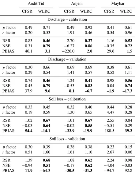
Table 5.Calibration and validation results of monthly CFSR- and WLRC-modelled discharge and soil loss. Values that meet at least the satisfactory criteria are highlighted in bold.

CFSR WLRC CFSR WLRC CFSR WLRC

Discharge – calibration

pfactor 0.49 0.71 0.49 0.92 0.41 0.61

rfactor 0.20 0.53 1.91 0.46 0.54 0.96

RSR 0.83 0.46 2.70 0.37 1.16 0.53

NSE 0.31 0.79 −6.27 0.86 −0.35 0.72

PBIAS 46.1 3.1 −226.0 2.0 29.6 1.5

Discharge – validation

pfactor 0.30 0.66 0.69 0.69 0.38 0.61

rfactor 0.29 0.54 1.41 0.57 0.52 1.11

RSR 0.74 0.46 1.24 0.41 0.98 0.56

NSE 0.45 0.79 −0.53 0.83 0.04 0.74

PBIAS 37.9 9.6 8.1 –6.7 –1.9 –17.3

Soil loss – calibration

pfactor 0.33 0.45 0.32 0.40 0.44 0.28

rfactor 0.19 0.59 1.30 0.65 4.47 0.28

RSR 1.02 0.67 1.01 0.67 2.55 0.84

NSE −0.03 0.64 −0.02 0.55 −5.51 0.29

PBIAS 54.4 –14.1 –33.9 –19.9 180.5 39.2

Soil loss – validation

pfactor 0.30 0.39 0.38 0.38 0.23 0.15

rfactor 0.51 1.60 1.61 1.10 2.67 0.06

RSR 1.39 0.68 1.08 0.62 2.24 0.98

NSE −0.94 0.51 −0.17 0.62 −4.04 −0.03

PBIAS 11.9 −64.3 –30.5 –31.3 −94.7 92.8

a general overestimation and unsatisfactory results for the CFSR data set with RSR: 1.39, NSE:−0.94, and satisfactory PBIAS:−11.9, indicating underestimation.

3.3.2 Anjeni

Soil loss modelling with WLRC rainfall data and calibrated discharge yielded satisfactory results. With apfactor of 0.40 and anrfactor of 0.65, and statistical parameters RSR: 0.67, NSE: 0.55, and PBIAS: −19.9, the model was just satis-factory. The graphic showed adequate results with a con-stant overestimation of the model except for 2 years in the early nineties. Modelling with CFSR data resulted in strongly unsatisfactory results (RSR: 1.01, NSE:−0.02, and PBIAS: −33.9), which can easily be explained with the strong model overestimation of rainfall and subsequently, discharge. Parameters could not be adapted further to achieve better results as they were already set to the edge of the pos-sible ranges.

Validation of sediment yield for Anjeni with WRLC data showed satisfactory results with RSR: 0.67, NSE: 0.64, and PBIAS:−14.1, indicating a general overestimation and un-satisfactory results for the CFSR data set with RSR: 1.02, NSE:−0.03, and satisfactory PBIAS:−1.9, indicating un-derestimation.

3.3.3 Maybar

Soil loss calibration with WLRC rainfall data and cali-brated discharge resulted in unsatisfactory statistical results (RSR: 1.24, NSE:−0.54, PBIAS:−34.1).pfactor andr fac-tor were 0.42 and 0.60, respectively.

(12)

dis-charge during belg and underestimation during kremt. This trend was redrawn with sediment calibration, resulting in small but distinct peaks during belg and smaller peaks than measured during kremt. There was no satisfactory calibration possible with CFSR rainfall data.

Validation of sediment yield for Maybar with WRLC data showed satisfactory results for both data sets with a very strong overestimation from the CFSR data set and an equally strong overestimation from the WLRC data set.

4 Conclusions

In this paper we studied the applicability of CFSR weather data to three small-scale watersheds in the Ethiopian High-lands with the goal of assessing the usability for future mod-elling in data-scarce regions. First, we compared CFSR and WLRC rainfall data at three stations in the Ethiopian High-lands and therefore rainfall data were compared on a monthly basis with box plots. Second, we modelled discharge with the SWAT model, once with WLRC data and once with CFSR rainfall data. Third, we modelled soil loss for the three sta-tions with the SWAT model and compared calibrated results to measured data. The WLRC rainfall data set resulted in three calibrated and validated discharge models, while the CFSR data resulted in none. For the soil loss modelling the WLRC rainfall data resulted in two out of three cali-brated and validated models while none could be adequately calibrated or validated for the CFSR data set. The SWAT modelling showed that CFSR rainfall pattern and rainfall yearly total amount variations were so significant that SWAT model calibration could not adequately represent measured discharge and sediment yield.

Our results clearly show that adequate discharge and soil loss modelling was not possible in the present case with the CFSR data. This suggests that SWAT simulations in small-scale watersheds in the Ethiopian Highlands do not perform well with CFSR data in every case, and that sometimes there is no substitute for high-quality conventional weather data. Such weather data – with high spatial and temporal climatic data resolution – were available for the three small-scale catchments used in the study but are not in many other cases. In these other cases, one should carefully check CFSR data against similar climatic stations with conventionally mea-sured data. In addition, discharge and soil loss modelling showed that usage of CFSR weather data not only resulted in substantial deviation in both total discharge and total soil loss, but also in the seasonal rainfall pattern. The seasonal weather pattern is one of the major drivers of soil loss and is especially pronounced in the Blue Nile Basin, with one long rainy season occurring as fields are ploughed and sown. Thus, contrary to previous studies for the Ethiopian High-lands, this study suggests that CFSR data may not be appli-cable in any case for small-scale modelling in data-scarce regions; the authors even suggest that outcomes of SWAT

modelling with CFSR data for small-scale catchments may yield erroneous results which cannot be verified and may lead to wrong conclusions. Nonetheless, the advantage of CFSR data is their completeness over time, which would al-low for comprehensive watershed modelling in regions with no conventional weather data or with longer gaps in conven-tionally recorded rainfall records.

Acknowledgements. The authors would like to thank the Centre for Development and Environment (CDE) of the University of Bern, Switzerland and the Water and Land Resource Centre in Addid Abeba, Ethiopia for providing data for this research and for their kind help in the field work in Ethiopia and the writing of this article.

Edited by: A. Guadagnini

References

Abbaspour, K. C.: SWAT-CUP 2012: SWAT calibration and uncer-tainty programs-A user manual, Tech. rep., Swiss Federal In-stitute of Aquatic Science and Technology, Eawag, Dübendorf, Switzerland, 2015.

Abbaspour, K. C., Johnson, C. A., and van Genuchten, M. T.: Es-timating Uncertain Flow and Transport Parameters Using a Se-quential Uncertainty Fitting Procedure, Vadose Zone J., 3, 1340– 1352, doi:10.2113/3.4.1340, 2004.

Abbaspour, K. C., Vejdani, M., Haghighat, S., and Yang, J.: SWAT-CUP Calibration and Uncertainty Programs for SWAT, in: The fourth International SWAT conference, Delft, the Netherlands, 1596–1602, 2007.

Alemayehu, T., Griensven, A., and Bauwens, W.: Evaluat-ing CFSR and WATCH Data as Input to SWAT for the Estimation of the Potential Evapotranspiration in a Data-Scarce Eastern-African Catchment, J. Hydrol. Eng., 05015028, doi:10.1061/(ASCE)HE.1943-5584.0001305, 2015.

Arnold, J. G., Srinivasan, R., Muttiah, R. S., and Williams, J. R.: Large area hydrologic modeling and assessment Part 1: model development, J. Am. Water Resour. Assoc., 34, 73–89, 1998. Arnold, J. G., Moriasi, D. N., Gassman, P. W., Abbaspour, K. C.,

White, M. J., Srinivasan, R., Santhi, C., Harmel, R. D., Van Griensven, A., Van Liew, M. W., Kannan, N., and Jha, M. K.: SWAT: Model use, calibration and validation, T. ASABE, 55, 1491–1508, 2012.

Belay, G.: Gerda Watershed Soil Report, Tech. Rep. February, Wa-ter and Land Resource Centre (WLRC), Addis Abeba, 2014. Betrie, G. D., Mohamed, Y. A., Van Griensven, A., Srinivasan, R.,

and Mynett, A.: Sediment management modelling in the Blue Nile Basin using SWAT model, Hydrol. Earth Syst. Sci., 15, 807– 818, doi:10.5194/hess-15-807-2011, 2011.

Bono, R. and Seiler, W.: The Soils of the Andit-Tid Research Unit (Ethiopia) Classification, Morphology and Ecology, with soil map 1 : 10’000, University of Bern, Bern, Switzerland, 1984. Bosshardt, U.: Catchment Discharge and Suspended Sediment

(13)

Bosshardt, U.: Hydro-sedimentological Characterisation of Kori Sheleko and Hulet Wenz Catchments, Maybar and Andit Tid Research Units, Soil Conservation Research Programme, Bern, Switzerland, 1999.

Cavazos, T. and Hewitson, B. C.: Performance of NCEP-NCAR re-analysis variables in statistical downscaling of daily precipita-tion, Clim. Res., 28, 95–107, 2005.

CFSR: Global Weather Data for SWAT, http://globalweather.tamu. edu/ (last access: 10 September 2014, 2016.

Chow, V. T.: Open-channel hydraulics, McGraw-Hill, Boston, MA, 1959.

De Almeida Bressiani, D., Srinivasan, R., Jones, C. A., and Mendiondo, E. M.: Effects of different spatial and temporal weather data resolutions on the stream flow modeling of a semi-arid basin, Northeast Brazil, Int. J. Agr. Biol. Eng., 8, 1–16, doi:10.3965/j.ijabe.20150803.970, 2015.

Dile, Y. T. and Srinivasan, R.: Evaluation of CFSR climate data for hydrologic prediction in data-scarce watersheds: an application in the Blue Nile River Basin, J. Am. Water Resour. Assoc., 50, 1226–1241, doi:10.1111/jawr.12182, 2014.

Diro, G. T., Grimes, D. I. F., Black, E., O’Neill, A., and Pardo-Iguzquiza, E.: Evaluation of reanalysis rainfall estimates over Ethiopia, Int. J. Climatol., 29, 67–78,doi:10.1002/joc.1699, 2009.

Douglas-Mankin, K., Srinivasan, R., and Arnold, J. G.: Soil and Wa-ter Assessment Tool (SWAT) Model: Current development and applications, Am. Soc. Agr. Biol. Eng., 53, 1423–1431, 2010. Faurès, J.-M., Goodrich, D. C., Woolhiser, D. A., and Sorooshian,

S.: Impact of small-scale spatial rainfall variability on runoff modeling, J. Hydrol., 173, 309–326, 2000.

Fuka, D. R., Walter, M. T., MacAlister, C., Degaetano, A. T., Steen-huis, T. S., and Easton, Z. M.: Using the Climate Forecast System Reanalysis as weather input data for watershed models, Hydrol. Process., 28, 5613–5623, doi:10.1002/hyp.10073, 2014. Gassman, P. W., Reyes, M. R., Green, C. H., and Arnold, J. G.:

The Soil and Water Assessment Tool: Historical development, applications, and future research directions, Am. Soc. Agr. Biol. Eng., 50, 1211–1250, 2007.

Gebremicael, T. G., Mohamed, Y. A., Betrie, G. D., van der Zaag, P., and Teferi, E.: Trend analysis of runoff and sediment fluxes in the Upper Blue Nile basin: A combined analysis of statistical tests, physically-based models and landuse maps, J. Hydrol., 482, 57–68, doi:10.1016/j.jhydrol.2012.12.023, 2013.

Gessesse, B., Bewket, W., and Bräuning, A.: Model-based charac-terization and monitoring of runoff and soil erosion in response to land use/land cover changes in the Modjo watershed, Ethiopia, Land Degrad. Dev., 26, 711–724, doi:10.1002/ldr.2276, 2014. Green, W. A. and Ampt, G. A.: Studies on Soil Phyics, J. Agricult.

Sci., 4, 1–24, doi:10.1017/S0021859600001441, 1911.

Hargreaves, G. H. and Samani, Z. A.: Reference crop evap-otranspiration from temperature, Appl. Eng. Agr., 2, 96–99, doi:10.13031/2013.26773, 1985.

Hurni, H.: Agroecologial belts of Ethiopia: Explanatory notes on three maps at a scale of 1 : 1,000,000, Soil Conservation Re-search Programme (SCRP), Centre for Development and Envi-ronment (CDE), Bern, Switzerland, 1998.

Kalnay, E., Kanamitsu, M., Kistler, R., Collins, W., Deaven, D., Gandin, L., Iredell, M., Saha, S., White, G., Woollen, J., Zhu, Y., Chelliah, M., Ebisuzaki, W., Higgins, W., Janowiak, J. E.,

Mo, K. C., Ropelewski, C., Wang, J., Leetmaa, A., Reynalds, R., Jenne, R., and Joseph, D.: The NCEP/NCAR 40-Year Reanalysis Project, B. Am. Meteorol. Soc., 77, 437–471, 1996.

Kejela, K.: The soils of the Anjeni Area – Gojam Research Unit, Ethiopia, University of Bern, Bern, Switzerland, 1995.

Kistler, R., Kalnay, E., Collins, W., Saha, S., White, G., Woollen, J., Chelliah, M., Ebisuzaki, W., Kanamitsu, M., Kousky, V., Dool, H. V. D., Jenne, R., and Fiorino, M.: The NCEP-NCAR 50-Year Reanalysis: Monthly Means CD-ROM and Documentation, B. Am. Meteorol. Soc., 82, 247–268, 2001.

Legates, D. R. and McCabe, G. J.: Evaluating the use of ’goodness-of-fit’ measures in hydrologic and hydrocli-matic model validation, Water Resour. Res., 35, 233–241, doi:10.1029/1998WR900018, 1999.

Lin, S., Jing, C., Chaplot, V., Yu, X., Zhang, Z., Moore, N., and Wu, J.: Effect of DEM resolution on SWAT outputs of runoff, sedi-ment and nutrients, Hydrol. Earth Syst. Sci. Discuss., 7, 4411– 4435, doi:10.5194/hessd-7-4411-2010, 2010.

Mbonimpa, E. G.: SWAT Model Application to Assess the Impact of Intensive Corn-farming on Runoff, Sediments and Phospho-rous loss from an Agricultural Watershed in Wisconsin, J. Water Resour. Protect., 04, 423–431, doi:10.4236/jwarp.2012.47049, 2012.

Moriasi, D. N., Arnold, J. G., Liew, M. W. V., Bingner, R. L., Harmel, R. D., and Veith, T. L.: Model evaluation guidelines for systematic quantification of accuracy in watershed simulations, Am. Soc. Agr. Biol. Eng., 50, 885–900, 2007.

Nash, J. E. and Sutcliffe, J. V.: River Flow Forecasting through Con-ceptual Models: Part 1. – A Discussion of Principles, J. Hydrol., 10, 282–290, 1970.

Neitsch, S. L., Arnold, J. G., Kiniry, J. R., and Williams, J. R.: Soil & Water Assessment Tool Theoretical Documentation Version 2009 Texas Water Resources Institute, SWAT, Technical Report No. 406, 1–647, 2011.

Poccard, I., Janicot, S., and Camberlin, P.: Comparison of rainfall structures between NCEP/NCAR reanalyses and ob-served data over tropical Africa, Clim. Dynam., 16, 897–915, doi:10.1007/s003820000087, 2000.

Saha, S., Moorthi, S., Pan, H.-L., Wu, X., Wang, J., Nadiga, S., Tripp, P., Kistler, R., Woollen, J., Behringer, D., Liu, H., Stokes, D., Grumbine, R., Gayno, G., Wang, J., Hou, Y.-T., Chuang, H.-Y., Juang, H.-M. H., Sela, J., Iredell, M., Treadon, R., Kleist, D., Van Delst, P., Keyser, D., Derber, J., Ek, M., Meng, J., Wei, H., Yang, R., Lord, S., Van Den Dool, H., Kumar, A., Wang, W., Long, C., Chelliah, M., Xue, Y., Huang, B., Schemm, J.-K., Ebisuzaki, W., Lin, R., Xie, P., Chen, M., Zhou, S., Higgins, W., Zou, C.-Z., Liu, Q., Chen, Y., Han, Y., Cucurull, L., Reynolds, R. W., Rutledge, G., and Goldberg, M.: The NCEP Climate Fore-cast System Reanalysis, B. Am. Meteorol. Soc., 91, 1015–1057, doi:10.1175/2010BAMS3001.1, 2010.

Schuol, J. and Abbaspour, K. C.: Using monthly weather statistics to generate daily data in a SWAT model ap-plication to West Africa, Ecol. Model., 201, 301–311, doi:10.1016/j.ecolmodel.2006.09.028, 2007.

SCRP and CDE: Digital Elevation Model (DEM) of Anjeni, Gojam, 2000a.

(14)

SCRP and CDE: Digital Elevation Model (DEM) of Maybar water-shed, Wello, 2000c.

Starks, P. J. and Moriasi, D. N.: Spatial resolution effect of precip-itation data on SWAT calibration and performance: implications for CEAP, Am. Soc. Agr. Biol. Eng., 52, 1171–1180, 2009. Stehr, A., Debels, P., and Romero, F.: Hydrological modelling with

SWAT under conditions of limited data availability: evaluation of results from a Chilean case study, Hydrolog. Sci. J., 53, 588–601, 2008.

Temesgen, M., Rockström, J., Savenije, H. H. G., Hoogmoed, W. B., and Alemu, D.: Determinants of tillage frequency among smallholder farmers in two semi-arid areas in Ethiopia, Phys. Chem. Earth, 33, 183–191, doi:10.1016/j.pce.2007.04.012, 2008. Tibebe, D. and Bewket, W.: Surface runoff and soil erosion estima-tion using the SWAT model in the Keleta Watershed, Ethiopia, Land Degrad. Dev., 22, 551–564, doi:10.1002/ldr.1034, 2011. USDA-SCS: Design Hydrographs, in: National Engineering

Hand-book, chap. 1–22, USDA Soil Conservation Service, Wash-ington, D.C., p. 824, http://www.nrcs.usda.gov/wps/portal/nrcs/ detailfull/national/water/?cid=stelprdb1043063 (ast access: 25 May 2015), 1972.

Wagner, P. D., Fiener, P., Wilken, F., Kumar, S., and Schneider, K.: Comparison and evaluation of spatial interpolation schemes for daily rainfall in data scarce regions, J. Hydrol., 464–465, 388– 400, doi:10.1016/j.jhydrol.2012.07.026, 2012.

Weigel, G.: The Soils of the Maybar Area, Wello Research Unit, Ethiopia, University of Bern, Bern, Switzerland, 1986.

Williams, J. R.: Flood routing with variable travel time or variable storage coefficients, T. ASABE, 12, 100–103, 1969.

Williams, J. R.: SPNM, a model for predicting sediment, phospho-rus, and nitrogen yields from agricultural basins, Water Resour. Bull., 16, 843–848, 1980.

Worqlul, A. W., Maathuis, B., Adem, A. A., Demissie, S. S., Lan-gan, S., and Steenhuis, T. S.: Comparison of rainfall estimations by TRMM 3B42, MPEG and CFSR with ground-observed data for the Lake Tana basin in Ethiopia, Hydrol. Earth Syst. Sci., 18, 4871–4881, doi:10.5194/hess-18-4871-2014, 2014.

Yang, Y., Wang, G., Wang, L., Yu, J., and Xu, Z.: Evaluation of Gridded Precipitation Data for Driving SWAT Model in Area Upstream of Three Gorges Reservoir, PLoS ONE, 9, e112725, doi:10.1371/journal.pone.0112725, 2014.

Yu, M., Chen, X., Li, L., Bao, A., and Paix, M. J. D. L.: Streamflow Simulation by SWAT Using Different Precipitation Sources in Large Arid Basins with Scarce Raingauges, Water Resour. Man-age., 25, 2669–2681, doi:10.1007/s11269-011-9832-z, 2011. Zeleke, G.: Landscape Dynamics and Soil Erosion Process