HESSD
12, 10651–10700, 2015The WACMOS-ET project – Part 2
D. G. Miralles et al.
Title Page
Abstract Introduction
Conclusions References
Tables Figures
◭ ◮
◭ ◮
Back Close
Full Screen / Esc
Printer-friendly Version Interactive Discussion
Discussion
P
a
per
|
Discussion
P
a
per
|
Discussion
P
a
per
|
Discussion
P
a
per
Hydrol. Earth Syst. Sci. Discuss., 12, 10651–10700, 2015 www.hydrol-earth-syst-sci-discuss.net/12/10651/2015/ doi:10.5194/hessd-12-10651-2015
© Author(s) 2015. CC Attribution 3.0 License.
This discussion paper is/has been under review for the journal Hydrology and Earth System Sciences (HESS). Please refer to the corresponding final paper in HESS if available.
The WACMOS-ET project – Part 2:
Evaluation of global terrestrial
evaporation data sets
D. G. Miralles1,2, C. Jiménez3, M. Jung4, D. Michel5, A. Ershadi6, M. F. McCabe6, M. Hirschi5, B. Martens2, A. J. Dolman1, J. B. Fisher7, Q. Mu8, S. I. Seneviratne5, E. F. Wood9, and D. Fernaìndez-Prieto10
1
Department of Earth Sciences, VU University Amsterdam, Amsterdam, the Netherlands
2
Laboratory of Hydrology and Water Management, Ghent University, Ghent, Belgium
3
Estellus, Paris, France
4
Max Planck Institute for Biogeochemistry, Jena, Germany
5
Institute for Atmospheric and Climate Science, ETH Zürich, Zürich, Switzerland
6
Division of Biological and Environmental Sciences and Engineering, King Abdullah University of Science and Technology, Thuwal, Saudi Arabia
7
Jet Propulsion Laboratory, California Institute of Technology, Pasadena, California, USA
8
Department of Ecosystem and Conservation Sciences, University of Montana, Missoula, Montana, USA
9
HESSD
12, 10651–10700, 2015The WACMOS-ET project – Part 2
D. G. Miralles et al.
Title Page
Abstract Introduction
Conclusions References
Tables Figures
◭ ◮
◭ ◮
Back Close
Full Screen / Esc
Printer-friendly Version Interactive Discussion
Discussion
P
a
per
|
Discussion
P
a
per
|
Discussion
P
a
per
|
Discussion
P
a
per
|
10
ESRIN, European Space Agency, Frascati, Italy
Received: 1 October 2015 – Accepted: 5 October 2015 – Published: 19 October 2015
Correspondence to: D. G. Miralles ([email protected])
HESSD
12, 10651–10700, 2015The WACMOS-ET project – Part 2
D. G. Miralles et al.
Title Page
Abstract Introduction
Conclusions References
Tables Figures
◭ ◮
◭ ◮
Back Close
Full Screen / Esc
Printer-friendly Version Interactive Discussion
Discussion
P
a
per
|
Discussion
P
a
per
|
Discussion
P
a
per
|
Discussion
P
a
per
Abstract
The WACMOS-ET project aims to advance the development of land evaporation es-timates at global and regional scales. Its main objective is the derivation, validation and inter-comparison of a group of existing evaporation retrieval algorithms driven by a common forcing data set. Three commonly used process-based evaporation
method-5
ologies are evaluated: the Penman–Monteith algorithm behind the official Moderate Resolution Imaging Spectroradiometer (MODIS) evaporation product (PM-MOD), the Global Land Evaporation Amsterdam Model (GLEAM), and the Priestley and Taylor Jet Propulsion Laboratory model (PT-JPL). The resulting global spatiotemporal variability of evaporation, the closure of regional water budgets and the discrete estimation of
10
land evaporation components or sources (i.e. transpiration, interception loss and di-rect soil evaporation) are investigated using river discharge data, independent global evaporation data sets and results from previous studies. In a companion article (Part 1), Michel et al. (2015) inspect the performance of these three models at local scales using measurements from eddy-covariance towers, and include the assessment the Surface
15
Energy Balance System (SEBS) model. In agreement with Part 1, our results here indi-cate that the Priestley and Taylor based products (PT-JPL and GLEAM) perform overall best for most ecosystems and climate regimes. While all three products adequately represent the expected average geographical patterns and seasonality, there is a ten-dency from PM-MOD to underestimate the flux in the tropics and subtropics. Overall,
20
results from GLEAM and PT-JPL appear more realistic when compared against surface water balances from 837 globally-distributed catchments, and against separate evapo-ration estimates from ERA-Interim and the Model Tree Ensemble (MTE). Nonetheless, all products manifest large dissimilarities during conditions of water stress and drought, and deficiencies in the way evaporation is partitioned into its different components. This
25
HESSD
12, 10651–10700, 2015The WACMOS-ET project – Part 2
D. G. Miralles et al.
Title Page
Abstract Introduction
Conclusions References
Tables Figures
◭ ◮
◭ ◮
Back Close
Full Screen / Esc
Printer-friendly Version Interactive Discussion
Discussion
P
a
per
|
Discussion
P
a
per
|
Discussion
P
a
per
|
Discussion
P
a
per
|
considering biome- or climate-specific composites of models. Yet, the generation of a multi-product ensemble, with weighting based on validation analyses and uncertainty assessments, is proposed as the best way forward in our long-term goal to develop a robust observational benchmark data set of continental evaporation.
1 Introduction
5
The importance of terrestrial evaporation (or “evapotranspiration”) for hydrology, agri-culture and meteorology has long been recognized. As a matter of fact, most of our understanding of the physics of evaporation originated in early experiments during the past two centuries (e.g. Dalton, 1802; Horton, 1919; Penman, 1948). However, it has been during the last decade that the interest of the scientific community towards land
10
evaporation has increased more dramatically, following the recognition of the key role it plays in climate (Wang and Dickinson, 2012; Dolman et al., 2014). Evaporation is highly sensitive to radiative forcing: changes in atmospheric chemical composition im-pact the magnitude of the flux, ensuring the propagation of anthropogenic forcing to all the components of the hydrological cycle (Wild and Liepert, 2010) and altering the
15
global availability of water resources (Hagemann et al., 2014). In addition, evaporation regulates climate through a series of feedbacks acting on air temperature, humidity and precipitation (Koster et al., 2006; Seneviratne et al., 2010), thus affecting climate trends (Douville et al., 2012; Sheffield et al., 2012) and hydro-meteorological extremes (Seneviratne et al., 2006; Teuling et al., 2013; Miralles et al., 2014a). Finally, due to the
20
link between transpiration and photosynthesis, atmospheric carbon concentrations and carbon cycle feedbacks are tightly linked to terrestrial evaporation (Reichstein et al., 2013). All together, evaporation stands as crucial nexus of processes and cycles in the climate system.
The rising interest of the climate community has coincided with an unprecedented
25
HESSD
12, 10651–10700, 2015The WACMOS-ET project – Part 2
D. G. Miralles et al.
Title Page
Abstract Introduction
Conclusions References
Tables Figures
◭ ◮
◭ ◮
Back Close
Full Screen / Esc
Printer-friendly Version Interactive Discussion
Discussion
P
a
per
|
Discussion
P
a
per
|
Discussion
P
a
per
|
Discussion
P
a
per
of direct in situ measurements, the scientific community have turned their eyes to-wards satellite remote sensing (Kalma et al., 2008; Wang and Dickinson, 2012; Dol-man et al., 2014). Consequently, different international activities now focus on the joint advancement of remote sensing technology and evaporation science, including the National Aeronautics and Space Administration (NASA) Energy and Water cycle
5
Study (NEWS, http://nasa-news.org), the European Union WATer and global CHange (WATCH, http://eu-watch.org) project, and the Global Energy and Water-cycle EXperi-ment (GEWEX) LandFlux initiative (http://wgdma.giss.nasa.gov/landflux.html). Despite continuing progress in the fields of remote sensing and computing science, up to date, the evaporative flux cannot be directly sensed from space; technology thus lags behind
10
our physical knowledge of evaporation. Nonetheless, taking advantage of this existing knowledge, different models have been proposed to combine the physical variables that are linked to the evaporation process and can be observed from space (e.g. radiation, temperature, soil moisture or vegetation dynamics). Such efforts have yielded a num-ber of global evaporation products in recent years (Mu et al., 2007; Zhang et al., 2010;
15
Fisher et al., 2008; Miralles et al., 2011b; Jung et al., 2010). These data sets are not to be interpreted as the direct result of satellite observations, but rather as model outputs generated based on satellite forcing data. The reader is directed to Su et al. (2011) or McCabe et al. (2013) for recent reviews of the state of the art.
Despite the recent initiatives dedicated to exploring these evaporation data sets –
20
LandFlux-EVAL in particular, see Jimenez et al. (2011) and Mueller et al. (2011, 2013) – the relative merits from each model at the global scale remain largely unexplored. To date, the lack of inter-model consistency in the choice of forcing data has hampered the attribution of the observed skill of each evaporation data set to differences in the models. Only recently, some efforts have been directed to homogenising the forcing
25
HESSD
12, 10651–10700, 2015The WACMOS-ET project – Part 2
D. G. Miralles et al.
Title Page
Abstract Introduction
Conclusions References
Tables Figures
◭ ◮
◭ ◮
Back Close
Full Screen / Esc
Printer-friendly Version Interactive Discussion
Discussion
P
a
per
|
Discussion
P
a
per
|
Discussion
P
a
per
|
Discussion
P
a
per
|
an consistent model inter-comparison at different spatial and temporal scales, and tar-geting the long-term goal of GEWEX LandFlux of achieving global closure of surface water and energy budgets. The project objectives strive to (a) develop a reference input data set consisting of satellite observations, reanalysis data and in situ measured me-teorology, (b) run a group of selected evaporation models forced by the reference input
5
data set, and (c) perform a cross-comparison, evaluation and validation exercise of the evaporation data sets that result from running this group of models. Four algorithms that are commonly used by the research community have been tested: the Surface En-ergy Balance Model, SEBS (Su, 2001); the Penman–Monteith approach that sets the basis for the official Moderate Resolution Imaging Spectroradiometer (MODIS)
evap-10
oration product, hereafter referred to as PM-MOD (Mu et al., 2007, 2011, 2013); the Global Land Evaporation Amsterdam Model, GLEAM (Miralles et al., 2011a, b); and the Priestley and Taylor model from the Jet Propulsion Laboratory, PT-JPL (Fisher et al., 2008).
In a companion article – henceforth referred to as Part 1 – Michel et al. (2015)
de-15
scribe the results of the local validation activities of WACMOS-ET based on in situ evaporation measurements from eddy-covariance towers. Here, we present the global-scale inter-product evaluation. After forcing the models with the reference input data set (see Sect. 2.2 for the description of the forcing data), the resulting evaporation data sets are evaluated by means of: (a) a general exploration of the global magnitude and
spa-20
tiotemporal variability of the estimates (Sects. 3.1 and 3.2), (b) a comparison to other, commonly-used, evaporation data sets (Sects. 3.1, 3.2 and 3.3), including the Model Tree Ensemble (MTE) estimates by Jung et al. (2009, 2010) and the European Cen-tre for Medium-range Weather Forecasts (ECMWF) Re-Analysis (ERA)-Interim data (Dee et al., 2011), (c) an assessment of the skill to close the surface water balance
25
HESSD
12, 10651–10700, 2015The WACMOS-ET project – Part 2
D. G. Miralles et al.
Title Page
Abstract Introduction
Conclusions References
Tables Figures
◭ ◮
◭ ◮
Back Close
Full Screen / Esc
Printer-friendly Version Interactive Discussion
Discussion
P
a
per
|
Discussion
P
a
per
|
Discussion
P
a
per
|
Discussion
P
a
per
et al., 2010), the current work concentrates on PM-MOD, GLEAM and PT-JPL, while the local-scale analysis in Part 1 also includes the SEBS model.
2 Methods and data
2.1 Models or algorithms
Here we present a brief description of the three models that are subjected to study
5
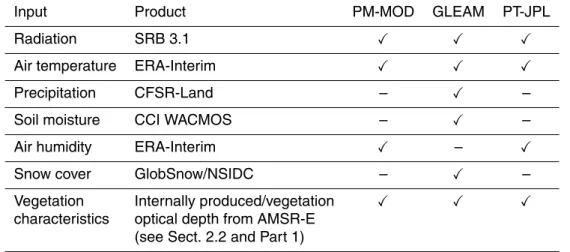
in this article. For more exhaustive descriptions the reader is directed to Part 1 and to the original articles describing the parameterizations and algorithms from PM-MOD (Mu et al., 2007, 2011), GLEAM (Miralles et al., 2011b; Martens et al., 2015) and PT-JPL (Fisher et al., 2008). A summary of the forcing requirements of PM-MOD, GLEAM and PT-JPL can be found in Table 1, together with the specific product for each input
10
variable.
2.1.1 PM-MOD
The Penman–Monteith model by Mu et al. (2007, 2011) is arguably the most widely used remote sensing-based global evaporation product and, in its latest version, it is also the algorithm behind the official MODIS (MOD16) product (Mu et al., 2013).
15
PM-MOD is based on the Monteith (1965) adaptation of Penman (1948), thus it is relatively high-demanding in terms of inputs. The parameterizations of aerodynamic and surface resistances for each component of evaporation are based on extending biome-specific conductance parameters to the canopy scale using vegetation phenol-ogy and meteorological data. The model applies the surface resistance scheme by
20
HESSD
12, 10651–10700, 2015The WACMOS-ET project – Part 2
D. G. Miralles et al.
Title Page
Abstract Introduction
Conclusions References
Tables Figures
◭ ◮
◭ ◮
Back Close
Full Screen / Esc
Printer-friendly Version Interactive Discussion
Discussion
P
a
per
|
Discussion
P
a
per
|
Discussion
P
a
per
|
Discussion
P
a
per
|
The non-consideration of wind speed appears as an advantage when aiming for a fully observation-driven product. As opposed to GLEAM and PT-JPL, which do not require calibration, the resistance parameters in PM-MOD have been calibrated with data from a set of global eddy-covariance towers (see Mu et al., 2011).
2.1.2 GLEAM
5
GLEAM is a simple land surface model fully dedicated to deriving evaporation based on satellite forcing only (Miralles et al., 2011b). It distinguishes between direct soil evaporation, transpiration from short and tall vegetation, snow sublimation, open-water evaporation, and interception loss from tall vegetation. The latter is independently cal-culated based on the Gash (1979) analytical model for interception forced by
observa-10
tions of precipitation (Miralles et al., 2010). The remaining components of evaporation are based upon the formulation by Priestley and Taylor (1972), which does not re-quire the parameterization of stomatal and aerodynamic resistances, in contrast to the Penman–Monteith equation. In the case of transpiration and soil evaporation, the po-tential evaporation estimates – resulting from the application of the Priestley and Taylor
15
approach – are constrained by a multiplicative stress factor. This dynamic stress factor is calculated based on the content of water in vegetation (microwave vegetation optical depth; Liu et al., 2011) and root-zone (multi-layer soil model driven by observations of precipitation and microwave surface soil moisture). The consideration of vegetation wa-ter content accounts for the effects of plant phenology, while the root-zone soil moisture
20
accounts for soil water stress. The model has been widely applied to look at trends in the water cycle (Miralles et al., 2014b) and land-atmospheric feedbacks (Guillod et al., 2015; Miralles et al., 2014a).
2.1.3 PT-JPL
The PT-JPL model by Fisher et al. (2008) uses the Priestley and Taylor (1972) approach
25
eco-HESSD
12, 10651–10700, 2015The WACMOS-ET project – Part 2
D. G. Miralles et al.
Title Page
Abstract Introduction
Conclusions References
Tables Figures
◭ ◮
◭ ◮
Back Close
Full Screen / Esc
Printer-friendly Version Interactive Discussion
Discussion
P
a
per
|
Discussion
P
a
per
|
Discussion
P
a
per
|
Discussion
P
a
per
physiological stress factors based on atmospheric moisture (vapour pressure deficit and relative humidity) and vegetation indices (normalized difference vegetation index, i.e. NDVI, and soil adjusted vegetation index) to constrain the atmospheric demand for water. This implies that the set of forcing requirements are in fact very comparable to those of PM-MOD (see Table 1). In order to partition land evaporation into soil
evap-5
oration, transpiration and interception loss, PT-JPL first distributes the net radiation to the soil and vegetation components, and then calculates the potential evaporation for soil, transpiration and interception separately. The partitioning between transpiration and interception loss is done using a threshold based on relative humidity. The model has been employed in a number of studies to estimate terrestrial evaporation at
re-10
gional and global scales in recent years (see e.g. Sahoo et al., 2011; Vinukollu et al., 2011a, b).
2.2 Input data
One of the objectives of the project has been to correct for a recurring issue in inter-product evaluations of global evaporation: due to inconsistencies in the forcing data
15
behind current evaporation products, it is difficult to attribute the observed inter-product disagreements to algorithm discrepancies (Jiménez et al., 2011; Mueller et al., 2013). Consequently, one of the first steps in WACMOS-ET has been to compile a reference input data set that has been used to run all models in a consistent manner. This con-sistency applies to both local-scale runs (in Part 1), and regional and global runs (in
20
the present study). On the other hand, since the required input variables are not the same for all models (see Table 1) – nor it is the models’ sensitivity to these input vari-ables and their uncertainties – it is not possible to fully attribute observed differences in performance to internal model errors. Nonetheless, our efforts to homogenize forcing data in a global evaporation inter-model comparison are unique, with the exception of
25
support-HESSD
12, 10651–10700, 2015The WACMOS-ET project – Part 2
D. G. Miralles et al.
Title Page
Abstract Introduction
Conclusions References
Tables Figures
◭ ◮
◭ ◮
Back Close
Full Screen / Esc
Printer-friendly Version Interactive Discussion
Discussion
P
a
per
|
Discussion
P
a
per
|
Discussion
P
a
per
|
Discussion
P
a
per
|
ing documents available in the project website. Nonetheless, a short summary is also provided here.
Some of the variables considered in the reference input data set have been inter-nally generated during the project, while others were selected from the existing pool of global climatic and environmental data sets. Choices regarding the spatial and
tem-5
poral resolution, period covered and study domain were made under the support of a large number of end users surveyed via internet (see project website). The targeted grid resolution of WACMOS-ET is 25 km, the domain is global and the study period spans 2005–2007. A 3 hourly temporal resolution maximizes the links to the work un-dertaken by the GEWEX LandFlux initiative to produce sub-daily evaporation estimates
10
(McCabe et al., 2015). The present Part 2 evaluates the outputs after aggregating them to daily, monthly and annual scales, while the skill of the models to resolve the diur-nal cycle of evaporation is explored in Part 1. Although the interdiur-nally generated input data sets were originally derived at a relatively fine (<5 km) resolution, critical inputs not generated within the project were only available at 75–100 km (see below).
Conse-15
quently, all input data sets have been spatially resampled to match the 25 km targeted resolution and re-projected into a common sinusoidal grid before using them to run the evaporation models.
Internally developed products include the fraction of photosynthetically active radia-tion and leaf area index, which are derived to a large extent from European satellites
20
(see Part 1). Data access, product descriptions and user guidelines for these data sets are available to interested parties upon request using the project website as gateway. Whereas PM-MOD and PT-JPL apply these internally generated data sets to charac-terize vegetation phenology, GLEAM uses observations of microwave optical depth as a proxy for vegetation water content, which is taken from the data set of Liu et al. (2011)
25
at 0.25◦ spatial resolution based on the Advanced Microwave Scanning Radiometer-Earth Observing System (AMSR)-E.
HESSD
12, 10651–10700, 2015The WACMOS-ET project – Part 2
D. G. Miralles et al.
Title Page
Abstract Introduction
Conclusions References
Tables Figures
◭ ◮
◭ ◮
Back Close
Full Screen / Esc
Printer-friendly Version Interactive Discussion
Discussion
P
a
per
|
Discussion
P
a
per
|
Discussion
P
a
per
|
Discussion
P
a
per
NASA/GEWEX Surface Radiation Budget (SRB) Release 3.1, which contains global 3 hourly averages of surface longwave and shortwave radiative fluxes on a 1◦resolution
grid. The SRB product is based on a range of satellite data, atmospheric reanalysis and data assimilation (Stackhouse et al., 2004). The meteorology (i.e. near-surface air temperature, air humidity and wind speed) comes from the ERA-Interim atmospheric
5
reanalysis, provided at 3 hourly resolution (using the forecast fields) and at a spatial resolution of ∼75 km. The reason for using atmospheric reanalysis data (based on observations assimilated into a weather forecast model), as opposed to direct satellite observations, is that some of these variables are presently difficult to observe over continents (like air temperature and humidity), if not impossible (like wind speed), and
10
are not routinely available at sub-daily time steps and over all weather conditions. Despite its relevance for plant-available water and interception loss, precipitation is not a direct input for most global satellite-based evaporation models. The same applies to surface soil moisture, which can also be observed from space. From the WACMOS-ET models, only GLEAM uses observations of precipitation and surface soil moisture
15
as input. In the reference input data set, precipitation data comes from the Climate Forecast System Reanalysis for Land (CFSR-Land, Coccia and Wood, 2015), which uses the Climate Prediction Center (CPC, Chen et al., 2008) and the Global Precip-itation Climatology Project (GPCP, Huffman et al., 2001) daily data sets and applies a temporal downscaling based on the CFSR (Saha et al., 2010). For soil moisture, we
20
use the satellite product of combined active-passive microwave surface soil moisture by Liu et al. (2012), which blends information from scatterometers and radiometers from different platforms, and was developed as part of the ESA Climate Change Initia-tive (CCI). In addition, GLEAM also uses information on snow water equivalents that is taken from the ESA GlobSnow product version 1.0 (Luojus and Pulliainen, 2010),
25
HESSD
12, 10651–10700, 2015The WACMOS-ET project – Part 2
D. G. Miralles et al.
Title Page
Abstract Introduction
Conclusions References
Tables Figures
◭ ◮
◭ ◮
Back Close
Full Screen / Esc
Printer-friendly Version Interactive Discussion
Discussion
P
a
per
|
Discussion
P
a
per
|
Discussion
P
a
per
|
Discussion
P
a
per
|
et al., 2003). Observations of soil moisture and snow water equivalents have a native resolution of 0.25◦and are imported in GLEAM at daily time steps.
2.3 Data used for evaluation
2.3.1 Other global land evaporation products
For the purpose of comparing our three WACMOS-ET products against related
evapo-5
ration data sets, we incorporate two additional data sets into the evaluation: the ERA-Interim reanalysis evaporation (Dee et al., 2011) and the MTE product (Jung et al., 2010, 2009). The latter is derived from satellite data and FLUXNET observations (Bal-docchi et al., 2001) using a machine-learning algorithm. In the model, tree ensembles are trained to predict monthly eddy-covariance fluxes based on meteorological, climate
10
and land cover data. It has a monthly temporal resolution and 0.5◦ spatial resolution.
For full details, the reader is referred to Jung et al. (2009).
2.3.2 Catchment water balance data
The mass balance of a catchment implies that the space and time integration of pre-cipitation (P) minus river runoff(Q) should equal evaporation (integrated over the same
15
space and time). This requires the consideration of a long period, so changes in stor-age within the catchment and travel time of precipitation through the landscape can be neglected (see discussion in Sect. 3.3). Given that river runoff and precipitation are more easily and extensively measured than evaporation, estimates ofP−Qbased on ground measurements of these two fluxes provide a convenient means to
evalu-20
ate evaporation over large domains and long periods (Liu et al., 2014; Miralles et al., 2011a; Vinukollu et al., 2011b; Sahoo et al., 2011). Here, we use globally-distributed multi-annual river discharge data for basins larger than 2500 km2. Discharge data and watershed boundaries are obtained from the Global RunoffData Centre (GRDC, 2013). Runoffdata have been converted from cumecs into mm yr−1 using the area of each
HESSD
12, 10651–10700, 2015The WACMOS-ET project – Part 2
D. G. Miralles et al.
Title Page
Abstract Introduction
Conclusions References
Tables Figures
◭ ◮
◭ ◮
Back Close
Full Screen / Esc
Printer-friendly Version Interactive Discussion
Discussion
P
a
per
|
Discussion
P
a
per
|
Discussion
P
a
per
|
Discussion
P
a
per
catchment as reported by the GRDC; basins where the absolute difference between the GRDC reported area and the area calculated from basin boundaries exceeded 25 % have been excluded from the analyses.
Precipitation for the target period 2005–2007 is taken from GPCP (Huffman et al., 2001) and the Global Precipitation Climatology Centre (GPCC) v6 (Schneider et al.,
5
2013). Two versions of GPCC v6 are processed by applying relative gauge correc-tion factors according to Fuchs et al. (2001) and Legates and Willmott (1990) to the native GPCC products as recommended by the producers. We further discard basins with (a priori) low-quality precipitation due to the low density of rain gauges (<0.1 per 0.5◦ latitude–longitude), frequent snowfall (>25 days per year based on CloudSat), or
10
where cumulative values of discharge exceed those of precipitation over the three-year period. Finally, net radiation data from the NASA Clouds and Earth’s Radiant Energy System (CERES) SYN1deg product (Wielicki et al., 2000) are used to exclude basins whereP−Qexceeds net radiation on average.
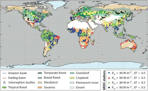
This results in a record of 837 basins from whichP−Qvalues are calculated. Figure 1
15
illustrates the location of the centroids of these catchments. Basins are then clustered in 30 classes based on log-transformed precipitation, net radiation, and evaporative fraction (i.e. evaporation over net radiation). This is done in order to reduce noise and retain clear patterns for evaluation. The clustering algorithm used is ak means with cityblock distance, with variables transformed to zero mean and unit variance. For
clar-20
HESSD
12, 10651–10700, 2015The WACMOS-ET project – Part 2
D. G. Miralles et al.
Title Page
Abstract Introduction
Conclusions References
Tables Figures
◭ ◮
◭ ◮
Back Close
Full Screen / Esc
Printer-friendly Version Interactive Discussion
Discussion
P
a
per
|
Discussion
P
a
per
|
Discussion
P
a
per
|
Discussion
P
a
per
|
3 Results and discussion
3.1 Global magnitude of terrestrial evaporation
The global mean annual volume of evaporation has been intensively debated in recent years (see e.g. Wang and Dickinson, 2012), with the range of reported global-averages in current CMIP5 models being large (Wild et al., 2014) and observational benchmark
5
data sets also differing significantly (Mueller et al., 2013). In this section, we aim to give some context to the global magnitude of evaporation that results from the WACMOS-ET analyses by contrasting the results against alternative evaporation data sets and existing literature. Unless otherwise noted, results come from aggregating the outputs from the 3 hourly global runs based on the 25 km spatial resolution of the reference
10
input data set for the period 2005–2007.
Overall, the total annual magnitude of evaporation estimated by the WACMOS-ET models amounts to 54.9×10³km3 for PM-MOD, 72.9×10³km3 for GLEAM and 72.5×10³km3 for PT-JPL. We further calculated 84.4×10³km3 for ERA-Interim and 68.3×10³km3for MTE based on the same 2005−2007 period. For comparison, values
15
typically found in literature based on a broad variety of methodologies and forcings are: 65.0×10³km3(Jung et al., 2010), 65.5×10³km3(Oki and Kanae, 2006), 65.8×10³km3 (Schlosser and Gao, 2010), 67.9×10³km3(Miralles et al., 2011a), 71×103km3 (Baum-gartner and Reichel, 1975), and 73.9×10³km3 (Wang-Erlandsson et al., 2014). We note that some of these studies considered the poles and desert regions, while
oth-20
ers did not; however, the contribution from these areas to the global means is rather marginal (<5 % of the total based on our analyses). Further, the study period consid-ered in WACMOS-ET is 2005−2007, while previously reported annual averages may be based on different periods.
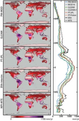
In Fig. 2 the multiannual (2005−2007) mean evaporation is displayed for the diff
er-25
HESSD
12, 10651–10700, 2015The WACMOS-ET project – Part 2
D. G. Miralles et al.
Title Page
Abstract Introduction
Conclusions References
Tables Figures
◭ ◮
◭ ◮
Back Close
Full Screen / Esc
Printer-friendly Version Interactive Discussion
Discussion
P
a
per
|
Discussion
P
a
per
|
Discussion
P
a
per
|
Discussion
P
a
per
right panel of Fig. 2. Model estimates are normally contained between the low values from PM-MOD and the high values from ERA-Interim; as an exception, PM-MOD can be comparatively high in Northern Hemisphere high latitudes (see Sect. 3.2). In Fig. 2, the latitudinal profiles from the original/official products from PM-MOD (i.e. MOD16), GLEAM (i.e. GLEAM v1) and PT-JPL (i.e. PT-Fisher) are also displayed for
compari-5
son. Note that the main differences between these official products and those devel-oped in WACMOS-ET relate to the choice of forcing – see Mu et al. (2013), Miralles et al. (2011a) and Fisher et al. (2008) for the particular forcing data used to gener-ate the official data sets. In addition, these models have been run here at sub-daily scale (three hourly) as opposed to their original daily (PM-MOD, GLEAM) or monthly
10
(PT-JPL) temporal resolutions. While for PM-MOD and PT-JPL the choice of temporal resolution and forcing in WACMOS-ET leads to overall lower values (see PM-MOD in tropics), for GLEAM, values are slightly higher than in the original version (v1).
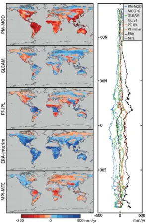
Inter-product differences in mean evaporation become more evident in Fig. 3, which presents the anomalies for each product calculated by subtracting the average of the
15
five-product ensemble. PM-MOD displays lower averages than the multi-product en-semble mean over the entire continental domain, with the exception of high-latitude regions, as discussed above. GLEAM shows higher than average values in Europe or Amazonia, and lower in North America. This pattern is somewhat shared by PT-JPL, although the two models disagree substantially in water-limited regions of Africa and
20
Australia, even if absolute mean values are low in those areas (see Fig. 2). This relates to the different model representation of evaporative stress, with GLEAM being based on observations of rainfall, surface soil moisture and vegetation optical depth, while PT-JPL is based on air humidity, maximum air temperature and NDVI. As mentioned in Sect. 2.2, it is important to note that even if we aimed to maximise consistency in
25
HESSD
12, 10651–10700, 2015The WACMOS-ET project – Part 2
D. G. Miralles et al.
Title Page
Abstract Introduction
Conclusions References
Tables Figures
◭ ◮
◭ ◮
Back Close
Full Screen / Esc
Printer-friendly Version Interactive Discussion
Discussion
P
a
per
|
Discussion
P
a
per
|
Discussion
P
a
per
|
Discussion
P
a
per
|
ERA-Interim values are often at the high end of predictions, consistent with the re-sults by Mueller et al. (2013), more than doubling the evaporation estimated by PM-MOD on some occasions (Fig. 2). MTE values, on the other hand, are lower than the inter-product average in the Himalayas and in tropical forests – which may potentially relate to the lack of a separate computation of interception loss and the long-lasting
5
question of whether interception can be measured with eddy-covariance instruments – but they agree well with the mean of the multi-product ensemble in other regions (Fig. 3). A quick overview on the range of uncertainty that can be expected may be obtained from the right panel of Fig. 3, where the latitudinal profiles of anomalies are illustrated. Data sets appear again to be confined between the low values of PM-MOD
10
and the high values of ERA-Interim. If that multi-model range is interpreted as an indi-cation of the uncertainty, it is worth noting that it may amount to 60–80 % of the mean evaporation, particularly in the subtropics. In the tropics, while the relative uncertainty is lower, the inter-product range still reaches∼500 mm yr−1according to the latitudinal profiles in Fig. 3. To put that volume into context, the mean annual evaporation is below
15
500 mm yr−1for more than 50 % of continental surfaces, according to the inter-product ensemble mean.
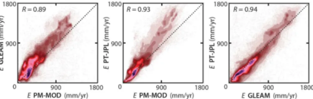
The spatial agreement among models is further explored in Fig. 4, which presents the spatial correlation for each pair of models based on their long-term global means (i.e. the maps in Fig. 2). Each land pixel is an independent point in the scatter. The lowest
20
spatial correlation occurs between PM-MOD and GLEAM (R=0.89), and the highest between GLEAM and PT-JPL (R=0.94). Although this may reflect the common choice of a Priestley and Taylor approach to calculate potential evaporation in GLEAM and PT-JPL, it occurs despite their large differences in input requirements (Table 1) and in the approach to derive evaporative stress and interception loss (Sect. 2.1). Yet, the
25
HESSD
12, 10651–10700, 2015The WACMOS-ET project – Part 2
D. G. Miralles et al.
Title Page
Abstract Introduction
Conclusions References
Tables Figures
◭ ◮
◭ ◮
Back Close
Full Screen / Esc
Printer-friendly Version Interactive Discussion
Discussion
P
a
per
|
Discussion
P
a
per
|
Discussion
P
a
per
|
Discussion
P
a
per
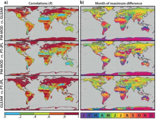
3.2 Temporal variability of terrestrial evaporation
In addition to long-term mean differences in evaporation, inter-product discrepancies in temporal dynamics are certainly expected. Temporal correlations based on the (2005– 2007) daily time series for each pair of models are illustrated in Fig. 5a. The overall agreement in temporal dynamics is larger in high latitudes and in the tropics, especially
5
between GLEAM and PT-JPL. In semiarid regions, product-to-product correlations are often below 0.5 and may drop below 0.2 (see e.g. low correlation between PM-MOD and PT-JPL in Australia), even if the large amplitude of the seasonal cycle in these transitional regimes could potentially lead to high temporal correlations. Overall, Fig. 5a corroborates that, although the agreement between GLEAM and PT-JPL is large, their
10
different approach to estimating water-availability constraints on evaporation and rain-fall interception loss leads to significant differences for semiarid regions and tropical forests.
Based on the monthly climatology of each model (calculated by averaging the esti-mates for the same month of the year considering the multi-year 2005–2007 period),
15
Fig. 5b illustrates the month in which the differences between a given pair of models are largest. In the Northern Hemisphere, the product-to-product differences are at their maximum during summertime, when the flux of evaporation is larger. This is particu-larly the case in comparisons to PM-MOD, given that the seasonal evaporation peak of PM-MOD is often less pronounced than for the other models (see also Figs. 6 and
20
7). In the tropics and the Southern Hemisphere, maximum differences between models occur at different times of the year, but often coincide with months of higher evaporative demand for water; this is the case for southern Africa, the Pampas region or Australia during the Austral summer.
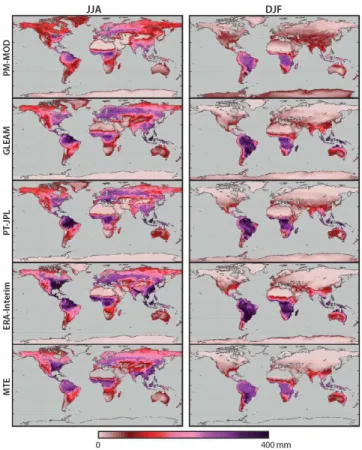
Figure 6 shows the average evaporation for boreal summer (JJA) and winter (DJF) for
25
HESSD
12, 10651–10700, 2015The WACMOS-ET project – Part 2
D. G. Miralles et al.
Title Page
Abstract Introduction
Conclusions References
Tables Figures
◭ ◮
◭ ◮
Back Close
Full Screen / Esc
Printer-friendly Version Interactive Discussion
Discussion
P
a
per
|
Discussion
P
a
per
|
Discussion
P
a
per
|
Discussion
P
a
per
|
by the availability of water. The lower values of PM-MOD are again highlighted. The underestimation of PM-MOD, with respect to the other two models, mostly occurs in times and locations for which both evaporative demand and water availability are high, thus evaporation is expected to be high as well (e.g. mid-latitude summer, tropics). However, PM-MOD is often higher than the other two models in periods and regions
5
where radiation is severely limited, potentially due to the underestimation of Priestley– Taylor type models (i.e. GLEAM and PT-JPL) when radiation is not the main supply of energy for evaporation (see e.g. Parlange and Katul, 1992), while the Penman– Monteith equation still considers adiabatic sources of energy to drive evaporation. Once more, differences in seasonal averages between GLEAM and PT-JPL may also exist
10
at the regional scale, especially in water-limited regimes, with Australia being a clear example (see also Fig. 8).
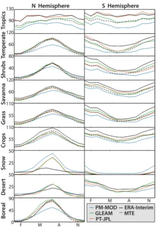
Nonetheless, Fig. 6 still shows a general agreement amongst the five models in their representation of seasonal dynamics. This agreement becomes also apparent in Fig. 7, which presents the seasonal monthly climatology of evaporation over different biome
15
types. Except for densely vegetated regions (see e.g. Southern Hemisphere tropical forests), artic regions or arid regimes (see e.g. Northern Hemisphere deserts), all mod-els capture similar monthly dynamics. This occurs despite the systematic differences in the absolute magnitudes of evaporation, which become again apparent – especially between PM-MOD and ERA-Interim – and may indicate limitations in the way that the
20
processes governing land evaporation are represented in our models. This highlights the importance of validation activities to improve and select algorithms.
Since the seasonal dynamics in evaporation are mostly dominated by the annual cy-cle of irradiance in nature (especially in energy-limited regions), the skill of these mod-els in correctly capturing these seasonal dynamics relies mostly on adequately
repre-25
HESSD
12, 10651–10700, 2015The WACMOS-ET project – Part 2
D. G. Miralles et al.
Title Page
Abstract Introduction
Conclusions References
Tables Figures
◭ ◮
◭ ◮
Back Close
Full Screen / Esc
Printer-friendly Version Interactive Discussion
Discussion
P
a
per
|
Discussion
P
a
per
|
Discussion
P
a
per
|
Discussion
P
a
per
extremes – and particularly droughts – being a target application of these models, cor-rectly reproducing the effect of surface water deficits on evaporation (and vice versa) appears crucial. One of the most remarkable hydro-meteorological extremes that coin-cide with the WACMOS-ET period is the Australian Millennium Drought, which affected (especially) southeastern Australia, and had in 2006 one of its most severe years of
5
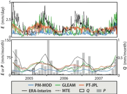
rainfall deficits (see van Dijk et al., 2013; Leblanc et al., 2012). Figure 8a shows the daily time series of evaporation for the Darling basin (area contoured in Fig. 1) from the three WACMOS-ET models during 2005–2007; ERA-Interim evaporation is also included for comparison. Figure 8b presents the monthly aggregates instead, and in-corporates the estimates of evaporation from MTE, precipitation from GPCC v6 (with
10
gauge correction factors from Fuchs et al., 2001) and river discharge data from GRDC. Given the arid conditions – especially pronounced during 2006 and 2007 – the mean annual runoff is very low, and the river in fact dries out completely for prolonged pe-riods (note also the more than two orders of magnitude difference between the right and left vertical axes in Fig. 8b). This indicates that almost the entire volume of
incom-15
ing rainfall is evaporated, thus cumulative evaporation should approximate cumulative precipitation over the multi-year period. We find, however, that in the case of all mod-els except for PM-MOD, evaporation is larger than the total rainfall for the three years: only 1 % higher for GLEAM, 10 % higher for PT-JPL, 16 % higher for MTE and 36 % higher for ERA-Interim. To some extent, this could reflect the progressive soil dry out
20
as the drought event evolves (i.e. the negative change in soil storage in time), or the accessibility of groundwater for root uptake (see e.g. Chen and Hu, 2004; Orellana et al., 2012), but in fact, there is a general tendency from all models to overestimate evaporation in drier catchments, as discussed in the following Sect. 3.3. Once more, Fig. 8 points that the estimates from the different products typically range between the
25
HESSD
12, 10651–10700, 2015The WACMOS-ET project – Part 2
D. G. Miralles et al.
Title Page
Abstract Introduction
Conclusions References
Tables Figures
◭ ◮
◭ ◮
Back Close
Full Screen / Esc
Printer-friendly Version Interactive Discussion
Discussion
P
a
per
|
Discussion
P
a
per
|
Discussion
P
a
per
|
Discussion
P
a
per
|
(see e.g. summer 2006), and the inter-product disagreement at short temporal scales (Fig. 8a) is considerably larger than the disagreement in mean seasonal cycles (Fig. 7).
3.3 Evaluation of evaporation based on the water balance closure
The skill of the different models to close the water budgets over 837 basins is inves-tigated here. As explained in Sect. 2.3.2, these analyses consist of a comparison of
5
modelled evaporation estimates from PM-MOD, GLEAM and PT-JPL (forced by the ref-erence input data set over 2005–2007) against estimates ofP−Q. Such a comparison implies the validity of a series of assumptions (see discussion below), but overall,P−Q estimates remain a valid, recursive means to evaluate long-term evaporation patterns (Liu et al., 2014; Miralles et al., 2011a; Vinukollu et al., 2011b; Sahoo et al., 2011).
10
Here, different criteria have been applied to ensure the quality of theP −Qestimates, and the remaining catchments (Fig. 1) have been clustered into 30 different classes based on average precipitation and evaporative fraction (see Sect. 2.3.2).
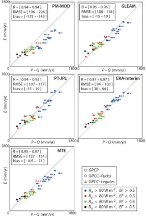
The skill of the three WACMOS-ET models to reproduce the general climatic patterns of evaporation becomes apparent from the scatterplots in Fig. 9. All three
WACMOS-15
ET products correlate well with the observations, which implies that their long-term spatial distribution of evaporation (Fig. 2) is overall realistic. The general negative bias of PM-MOD becomes again discernible when compared to theP −Qdata, which is in agreement with the results by Mu et al. (2013). In addition, there is a tendency from all models to underestimate evaporation in wet regions and overestimate in dry regions
20
– the latter was already suggested in Fig. 8. While, this pattern could potentially be explained by systematic errors inP−Q(see discussion below on the possible sources of errors when consideringP −Qas a proxy for evaporation), the same tendency has been found in Part 1 in comparisons against independent eddy-covariance towers. Once more, it is interesting to see how the independent evaporation data sets, i.e.
25
HESSD
12, 10651–10700, 2015The WACMOS-ET project – Part 2
D. G. Miralles et al.
Title Page
Abstract Introduction
Conclusions References
Tables Figures
◭ ◮
◭ ◮
Back Close
Full Screen / Esc
Printer-friendly Version Interactive Discussion
Discussion
P
a
per
|
Discussion
P
a
per
|
Discussion
P
a
per
|
Discussion
P
a
per
MTE) are again highlighted, together with the tendency to overestimate evaporation in dry catchments and underestimate in wet ones, which shared by all five data sets.
As mentioned above, the use of P −Q as a benchmark for evaporation depends on the validity of several assumptions. First, the catchment needs to be watertight (no sub-surface leakage to other catchments) and its geographical boundaries must be well
5
defined. Second, the entire volume of river water that is extracted for direct human use must return to the river, and it shall do so upstream of the staffgauge location. Third, the lag-time between rainfall events and the discharge measured at the station can be neglected when compared to the total period of study. Finally, the changes in soil water storage within the catchment should be insignificant compared to the cumulative
10
volume of the three main hydrological fluxes. Here, by considering long-term averages
of P −Q, these assumptions appear to be reasonable for most continental regions.
However, for industrialised areas with dense population, the consumption and export of water and the human regulation of the reservoir storages may compromise these as-sumptions. Nonetheless, the largest sources of uncertainty regarding the use ofP −Q
15
as estimate of catchment evaporation likely come from (a) the definition of the runoff -contributing area, and (b) errors in precipitation and discharge observations. In fact, Fig. 9 shows that the choice of precipitation product can have a significant influence in the results, even despite the existing inter-dependencies between the gauge-based precipitation data sets tested here (Sect. 2.3.2). On the other hand, uncertainties in
20
observations of river runoffcan also be significant, and come from errors in the mea-surements of river height, the discharge data used to calibrate the rating curves, or the interpolation and extrapolation due to changes in riverbed roughness, hysteresis ef-fects, etc. (see e.g. Di Baldassarre and Montanari, 2009). Finally, it is important to note that model estimates correspond to the period 2005–2007, while P−Qestimates do
25
HESSD
12, 10651–10700, 2015The WACMOS-ET project – Part 2
D. G. Miralles et al.
Title Page
Abstract Introduction
Conclusions References
Tables Figures
◭ ◮
◭ ◮
Back Close
Full Screen / Esc
Printer-friendly Version Interactive Discussion
Discussion
P
a
per
|
Discussion
P
a
per
|
Discussion
P
a
per
|
Discussion
P
a
per
|
Additionally, the fit of the models to a Budyko curve (Budyko, 1974) is explored in Fig. 10 as a general diagnostic for the robustness of mean evaporation estimates and their consistency with the input of water and energy. Potential evaporation estimates are taken from the corresponding models and precipitation from the GPCC v6 product with gauge correction factors from Fuchs et al. (2001), to be consistent with Figs. 8 and
5
9. Overall, results are in agreement with the water balance scatterplots (Fig. 9). The fraction of precipitation that is evaporated (E/P) is usually lower for PM-MOD; however, this does not happen due to an underestimation of the atmospheric demand for water, as the values of the ratio of potential evaporation over precipitation (Ep/P) are overall comparable to those from GLEAM and PT-JPL. The PM-MOD product has therefore
10
a general tendency to overestimate the surface evaporative stress (i.e. underestimate the ratio E/Ep), which may explain the overall lower estimates of evaporation found across our analyses. GLEAM and PT-JPL show a better fit to the Budyko diagram, and a transition from arid to wet climates that is consistent with the average fluxes of precipitation and net radiation. Nevertheless, it is worth noting that all three models
es-15
timate average values of evaporation that overcome average precipitation in numerous locations.
3.4 Partitioning of evaporation into separate components
The flux of land evaporation results from the summation of three main components or sources: (a) transpiration (the process that describes the movement of water from the
20
soil, through the plant xylem, to the leaf and finally to the atmosphere), (b) interception loss (the vaporization of the volume of water that is held by the surface of vegeta-tion during rainfall), and (c) soil evaporavegeta-tion (the direct vaporizavegeta-tion of water from the topsoil). These processes require separate consideration in our models due to their differences in bio-physical drivers and rates (Savenije, 2004; Dolman et al., 2014). In
25
HESSD
12, 10651–10700, 2015The WACMOS-ET project – Part 2
D. G. Miralles et al.
Title Page
Abstract Introduction
Conclusions References
Tables Figures
◭ ◮
◭ ◮
Back Close
Full Screen / Esc
Printer-friendly Version Interactive Discussion
Discussion
P
a
per
|
Discussion
P
a
per
|
Discussion
P
a
per
|
Discussion
P
a
per
Transpiration is the component that has received the most attention by the scientific community in recent years, due to its connection to different biogeochemical cycles. The global contribution of transpiration to total average evaporation has been exten-sively debated recently (Schlesinger and Jasechko, 2014; Wang et al., 2014). Studies have reported values ranging between 35–90 %, based on isotopes (Jasechko et al.,
5
2013; Coenders-Gerrits et al., 2015), sap-flow measurements (Moran et al., 2009), satellite data (Miralles et al., 2011a; Mu et al., 2011) or modelling (Wang-Erlandsson et al., 2014). Consequently, this large range of uncertainty is also expected in the rel-ative contribution from other evaporation sources. Moreover, reducing this uncertainty appears particularly challenging due to the limited amount of ground data that can be
10
used for validation and the nature of the techniques used to measure latent heat flux: most measuring techniques (e.g. lysimeters, eddy-covariance instruments, scintillome-ters) cannot distinguish amongst the different sources of evaporation.
All three WACMOS-ET models estimate the components of evaporation separately. In the case of PT-JPL and PM-MOD, the available energy is partitioned into the different
15
land covers to estimate the contribution from each of them. The approach in GLEAM is somewhat different, as the flux of interception loss is calculated using a different algorithm that the one used for transpiration and soil evaporation. Figure 11 illustrates the average contribution of each evaporation component to the total flux as estimated by the WACMOS-ET models. In the case of GLEAM (which calculates sublimation
20
separately), the flux from snow and ice has been added to the bare soil evaporation in this figure to allow comparison to the other two products.
The discrepancy amongst modelled evaporation components show in Fig. 11 is large, and calls for a thorough validation of the way the contribution from different sources is estimated, and even a revision to ensure that the conceptual definition of
25
com-HESSD
12, 10651–10700, 2015The WACMOS-ET project – Part 2
D. G. Miralles et al.
Title Page
Abstract Introduction
Conclusions References
Tables Figures
◭ ◮
◭ ◮
Back Close
Full Screen / Esc
Printer-friendly Version Interactive Discussion
Discussion
P
a
per
|
Discussion
P
a
per
|
Discussion
P
a
per
|
Discussion
P
a
per
|
ponent. In tropical forests, the direct soil evaporation can also exceed transpiration in the case of PM-MOD, while for GLEAM and PT-JPL bare-soil evaporation is almost in-existent. The mean inter-model disagreement is manifest in the pie diagrams in Fig. 11, with GLEAM estimating a large contribution from transpiration (76 %) and low from soil evaporation (14 %), PM-MOD estimating little transpiration (24 %) and a large
contri-5
bution from soil evaporation (52 %), and both PM-MOD and PT-JPL yielding a much larger flux of interception loss than GLEAM. Nevertheless, and as discussed above, recent reviews have revealed comparable levels of uncertainty based on a wide range of independent methods (Schlesinger and Jasechko, 2014; Wang et al., 2014).
While the global contribution of transpiration has received much attention in literature
10
(Jasechko et al., 2013; Coenders-Gerrits et al., 2015), the flux of interception loss has seldom been explored globally (Miralles et al., 2010; Vinukollu et al., 2011b; Wang-Erlandsson et al., 2014). The physical process of interception loss differs from that of transpiration on its sensitivity to environmental and climatic variables: the rates and magnitude of interception are dictated by the aerodynamic properties of the vegetation
15
stand, and the occurrence and characteristics of rainfall (Horton, 1919). In fact, while solar radiation is normally the main supply of energy for transpiration and soil evap-oration (Wild and Liepert, 2010), the source of energy powering interception loss is still debated (Holwerda et al., 2011). The limited process understanding, together with the scarcity of ground measurements for validation, makes interception loss
particu-20
larly challenging to model. Nonetheless, interception has often been reported in units of percentage of incoming rainfall during the restricted number of past in situ cam-paigns (see e.g. Miralles et al. (2010) for a non-exhaustive list of these camcam-paigns). This makes interception measurements easy to extrapolate in time and space, and it allows for a relatively straightforward validation of the estimates from our three models.
25
HESSD
12, 10651–10700, 2015The WACMOS-ET project – Part 2
D. G. Miralles et al.
Title Page
Abstract Introduction
Conclusions References
Tables Figures
◭ ◮
◭ ◮
Back Close
Full Screen / Esc
Printer-friendly Version Interactive Discussion
Discussion
P
a
per
|
Discussion
P
a
per
|
Discussion
P
a
per
|
Discussion
P
a
per
PM-MOD and PT-JPL there is over a two-fold overestimation of the mean flux. Tempo-ral dynamics of interception loss from the three products do not correlate well either, as GLEAM tends to follow the occurrence of rainfall, while PM-MOD and PT-JPL are more affected by net radiation variability, as expected from the algorithms (i.e. Gash’s model for GLEAM, Penman–Monteith for PM-MOD and Priestley and Taylor for PT-JPL).
5
Further analyses are needed to explore the skill of these (and other) models to sep-arately derive the different evaporation components or sources. Nevertheless, these preliminary analyses point at the need for caution when using global estimates of tran-spiration, soil evaporation or interception loss from a single model in isolation, as the disagreements can be much larger than for total land evaporation. Up to date, the lack
10
of in situ networks that measure the components of evaporation independently remains an inexorable bottleneck for the improvement of model estimates.
4 Conclusions
The ESA WACMOS-ET project started in 2012 with the goal of performing a cross-comparison and validation exercise of a group of selected global observational
evapo-15
ration algorithms driven by a consistent set of forcing data. With the project coming to an end, this article has focussed on the global and regional evaluation of the resulting evaporation products.
The three main products scrutinised here were the Penman–Monteith approach from the official MODIS evaporation product (Mu et al., 2007, 2011, 2013), GLEAM (Miralles
20
et al., 2011a, b; Martens et al., 2015) and the Priestley–Taylor JPL model (Fisher et al., 2008); the SEBS model (Su, 2001), which was analysed at the local scale in Part 1 (re-vealing good performance in terms of correlations but a systematic overestimation of evaporation), was not evaluated in this contribution. The spatiotemporal magnitude and variability of the three global evaporation products were compared to analogous
esti-25
HESSD
12, 10651–10700, 2015The WACMOS-ET project – Part 2
D. G. Miralles et al.
Title Page
Abstract Introduction
Conclusions References
Tables Figures
◭ ◮
◭ ◮
Back Close
Full Screen / Esc
Printer-friendly Version Interactive Discussion
Discussion
P
a
per
|
Discussion
P
a
per
|
Discussion
P
a
per
|
Discussion
P
a
per
|
the water balance over 837 river basins worldwide, and the model partitioning of evap-oration into different components have also been explored.
Despite our efforts to create a homogeneous forcing data set to run the evaporation models, the input requirements of each model are different, which implies that the resulting inter-product disagreements are the result of both internal differences in the
5
models, and uncertainties in forcing and ancillary data. This prevents us from making strong claims about the quality of the models. However, there is also a list of take-home messages to learn from these analyses:
– In agreement with the local-scale validation in Part 1, the PM-MOD product tends to underestimate evaporation (see e.g. Figs. 3 and 9). This underestimation is
sys-10
tematic, being larger in absolute terms in the tropics (where evaporation is larger), and larger in relative terms in drier subtropical regions (Fig. 3). As an exception, in high latitudes PM-MOD estimates are greater than those from GLEAM and PT-JPL; this may reflect known deficiencies in Priestley–Taylor-based approaches over conditions of low available energy (see e.g. Parlange and Katul, 1992).
15
– The global average magnitude of evaporation from GLEAM and PT-JPL agree well with each other and with the envelope of literature values (see Figs. 2 and 4). This agreement extends to the average latitudinal patterns, which lay between those of PM-MOD and ERA-Interim (Figs. 2 and 3). In terms of temporal dy-namics, there are differences between GLEAM and PT-JPL in dry conditions, as
20
expected from their distinctive approach at representing evaporative stress (see Sect. 2.1). These differences are pronounced in the Southern Hemisphere sub-tropics (Fig. 5a), reflect more clearly in daily anomalies than in seasonal cycles (Fig. 7), and may exacerbate during specific drought events (Fig. 8).
– The partitioning of evaporation into different components is a facet of these
mod-25
compo-HESSD
12, 10651–10700, 2015The WACMOS-ET project – Part 2
D. G. Miralles et al.
Title Page
Abstract Introduction
Conclusions References
Tables Figures
◭ ◮
◭ ◮
Back Close
Full Screen / Esc
Printer-friendly Version Interactive Discussion
Discussion
P
a
per
|
Discussion
P
a
per
|
Discussion
P
a
per
|
Discussion
P
a
per
nents may fluctuate substantially (Fig. 11). As an example, differences in intercep-tion loss amongst models (Fig. 12) may explain a large part of the disagreements in the seasonality of evaporation over tropical forests (Fig. 7). Further exploring the skill of the models at partitioning evaporation into its different sources remains a critical task for the future. This is outside the scope of WACMOS-ET and it
5
would require innovative means of validation beyond traditional comparisons to eddy-covariance and lysimeter data.
– On a more positive note, the analysis of the skill of different models to close the water balance over particular catchments reveals that the general climatic pat-terns of evaporation are well captured by all models (Fig. 9). While this
compar-10
ison has also unveiled the general underestimation by PM-MOD (and overesti-mation by ERA-Interim), all products correlate well with the cumulative values
ofP −Q. We stress however that this agreement does not indicate whether the
multi-scale temporal dynamics of evaporation are well captured. For a thorough validation of evaporation temporal variability, we direct the readers to Part 1.
15
In summary, the activities in WACMOS-ET have demonstrated that some of the exist-ing evaporation models and products require an in-depth scrutiny to correct for sys-tematic errors in their estimates. This is especially the case over semi-arid regions and tropical forests. In addition, even models that have demonstrated a more robust per-formance, like GLEAM and PT-JPL, may differ substantially from one another under
20
certain biomes and climates. Overall, our results imply the need for caution in using a single model for any large-scale application in isolation, especially in studies in which transpiration, soil evaporation or interception loss are investigated separately.
As remote sensing science continues advancing, new long-term records of physical variables to constrain these models are becoming available (e.g. chlorophyll
fluores-25
HESSD
12, 10651–10700, 2015The WACMOS-ET project – Part 2
D. G. Miralles et al.
Title Page
Abstract Introduction
Conclusions References
Tables Figures
◭ ◮
◭ ◮
Back Close
Full Screen / Esc
Printer-friendly Version Interactive Discussion
Discussion
P
a
per
|
Discussion
P
a
per
|
Discussion
P
a
per
|
Discussion
P
a
per
|
models may perform better under certain conditions (Ershadi et al., 2014; McCabe et al., 2015). For an inter-product merger to add new skill, the sensitivity of each model to its forcing should be further explored, and a robust propagation of uncertainties ap-pears essential to merge these products efficiently.
The reader is directed to additional supporting documents available form the project
5
website at http://WACMOS-ET.estellus.eu.
Author contributions. D. G. Miralles, C. Jiménez, M. Jung, D. Michel, A. Ershadi, M. F. McCabe, M. Hirschi and D. Fernaìndez-Prieto designed the content of the manuscript. D. G. Miralles, C. Jiménez and M. Jung did the analyses. D. G. Miralles wrote the paper. J. B. Fisher and Q. Mu provided the computer codes of the PT-JPL and PM-MOD models, respectively. All
10
authors contributed to the accomplishment of the project, and the discussion and interpretation of results.
Acknowledgements. This work was undertaken as part of the European Space Agency (ESA) project WACMOS-ET (Contract No. 4000106711/12/I-NB). Discharge data were provided by the Global Runoff Data Centre, 56068 Koblenz, Germany. We thank Ulrich Weber and Eric
15
Thomas for processing the catchment data. D. G. Miralles acknowledges the financial support from the Netherlands Organization for Scientific Research through grant 863.14.004, and the Belgian Science Policy Office (BELSPO) in the frame of the STEREO III programme, project SAT-EX (SR/00/306). A. Ershadi and M. F. McCabe acknowledge funding from the King Abdul-lah University of Science and Technology. J. B. Fisher acknowledges funding under the NASA
20