OPTIMIZATION STOCK PORTFOLIO WITH MEAN-VARIANCE
AND LINEAR PROGRAMMING:
CASE IN INDONESIA STOCK MARKET
Yen Sun
Accounting Department, Faculty of Economics and Business, Bina Nusantara University Jln. K.H. Syahdan No. 9, Palmerah, Jakarta Barat 11480
ABSTRACT
It is observed that the number of Indonesia’s domestic investor who involved in the stock exchange is very less compare to its total number of population (only about 0.1%). As a result, Indonesia Stock Exchange (IDX) is highly affected by foreign investor that can threat the economy. Domestic investor tends to invest in risk-free asset such as deposit in the bank since they are not familiar yet with the stock market and anxious about the risk (risk-averse type of investor). Therefore, it is important to educate domestic investor to involve in the stock exchange. Investing in portfolio of stock is one of the best choices for risk-averse investor (such as Indonesia domestic investor) since it offers lower risk for a given level of return. This paper studies the optimization of Indonesian stock portfolio. The data is the historical return of 10 stocks of LQ 45 for 5 time series (January 2004 – December 2008). It will be focus on selecting stocks into a portfolio, setting 10 of stock portfolios using mean variance method combining with the linear programming (solver). Furthermore, based on Efficient Frontier concept and Sharpe measurement, there will be one stock portfolio picked as an optimum Portfolio (Namely Portfolio G). Then, Performance of portfolio G will be evaluated by using Sharpe, Treynor and Jensen Measurement to show whether the return of Portfolio G exceeds the market return. This paper also illustrates how the stock composition of the Optimum Portfolio (G) succeeds to predict the portfolio return in the future (5th January – 3rd April 2009). The result of the study observed that optimization portfolio using Mean-Variance (consistent with Markowitz theory) combine with linear programming can be applied into Indonesia stock’s portfolio. All the measurements (Sharpe, Jensen, and Treynor) show that the portfolio G is a superior portfolio. It is also been found that the composition (weights) stocks of optimum portfolio (G) can be used to predict the forward return (5th January – 3rd April 2009). It is shown that the stock portfolio return of 5th January – 3rd April 2009) has exceeded the market return for the same period of time based on Sharpe and Treynor measurement.
Keywords: optimum portfolio, mean-variance, linear programming, LQ45, performance evaluation
ABSTRAK
karena itu, sangatlah penting untuk mengedukasi investor domestik agar mereka dapat berperan dalam kegiatan pasar modal. Investasi dalam stock portofolio adalah salah satu pilihan investasi yang cukup bagus untuk tipe investor risk – averse (seperti tipe investor domestik yang ada di Indonesia) karena investasi tersebut menawarkan resiko yang lebih rendah untuk tingkat return tertentu. Paper ini mempelajari tentang optimisasi stock portofolio di Indonesia. Data yang digunakan adalah data return historis selama 5 tahun dari 10 stock yang terdaftar di LQ 45 (periode Januari 2004 – Desember 2008). Paper ini akan berfokus pada pemilihan stock untuk portofolio, pembentukan 10 stock portofolio dengan menggunakan metode Mean Variance yang dikombinasikan dengan linear programming (solver). Dari 10 stock portofolio tersebut akan terpilih satu stock portofolio (Portfolio G) yang optimum berdasarkan efficient frontier dan metode Sharpe. Langkah selanjutnya, performance dari Portofolio G akan dievaluasi apakah lebih baik dari Return market dengan metode Sharpe, Treynor dan Jensen. Tulisan ini juga akan mengilustrasikan bagaimana komposisi stock dari portofolio G yang optimum berhasil memprediksi tingkat pengembalian portofolio di masa depan (periode 5 Januari – 3 April 2009). Hasil dari studi ini menemukan bahwa optimisasi portofolio menggunakan Mean-Variance (konsisten dengan teori Markowitz) yang dikombinasikan dengan linear programming dapat diaplikasikan ke Indonesia stock portofolio. Semua metode pengukuran (Sharpe, Jensen, dan Treynor) menunjukkan bahwa portofolio G adalah portfolio yang superior. Pun telah ditemukan bahwa komposisi stock dalam portofolio G yang optimum dapat digunakan untuk memprediksi return di masa yang akan datang (periode 5 Januari – 3 April 2009) karena tingkat return yang dihasilkan periode tersebut melebihi tingkat return market untuk periode yang sama berdasarkan pengukuran Sharpe dan treynor.
Kata kunci: portofolio optimal, mean-variance, linear programming, LQ45, evaluasi kinerja
INTRODUCTION
In 2009, Indonesia was the third country in Asia which has the highest economy growth after China and India. This has to be supported by its capital market activity. Indonesia’s Capital market called Indonesia Stock Exchange (IDX). Indonesia Stock Exchange (IDX) has grown rapidly since the automatic trading system has been applied on 25th May 1995. The entire economic indicator such as transaction frequency and volume has increased substantially. The average transaction in 2007 has reached Rp. 4.3 trillion per day. It continued to increase until the first semester in 2008 to Rp. 5.6 trillion. In the second semester, there was a decline in transaction volume as an impact of USA Sub prime Crisis, but the average transaction in 2008 was still higher than 2007 about Rp. 4.5 trillion. Compare to 1994 before the automatic trading, the transaction volume was merely about Rp. 104 billion per day, which means that in 14 years the average transaction has soared by approximately 4,000%.
Despite the growth of transaction activity, the Jakarta Composite Index or JSX Composite also has increased significantly. It can be noted that JSX Composite was still at 469.640 in 1994, but it continued to increase until decreasing in 1997 affected by the Asian Monetary crisis. However, in 2000 and so on, it persisted to rise again and reached the peak on January 2008 at level 2,830.263 or increased by 502.65% compared to 1994 level (Indonesia Stock Exchange, 2008).
Indonesia’s economy, the foreign investor will tend to draw its fund from the market. This action will be followed by domestic investor. Consequently, the stock price will drop. Dropped price affects the speculator to chase dollar and depreciates Rupiah. A significant depreciation will distress and decelerate the economic condition of a country. For instance, the price of raw materials for import will be higher and affect to higher production cost. Moreover, Rupiah depreciation will remind investor on monetary crisis in 1997-1998, because the crisis occurred due to the depreciation of Rupiahs. Uncertainties will make consumers to lessen their consumption resulting a slow economy. Thus, it can be stated that instability of Indonesia Stock Exchange impacts to the Indonesia’s economy (Sadewa, 2009).
Indonesia Stock Exchange is highly affected by foreign investor due to the small number of domestic investor. In 2009, it is approximately 300.000 investor (only about 0.1% from total population number) which is fewer than other Asian countries such as Singapore (about1.26 million people or 30% from total population), and Malaysia (about 3 million people or 12.8% from total population).
There are also small contribution numbers of stock market to Indonesia’s economy. In 2008, the market capitalization of Stock Exchange was only 21.7% from the Gross Domestic Bruto. This number is much smaller from Singapore (148%), Thailand (39.2%), and Malaysia (89.6%). It also indicates the number of companies have involved in the stock market. It means that the number of Indonesia’s company listed in the IDX is relatively smaller than other country. It is noted that by 2008, listed company is only about 396 companies which is smaller compares to Singapore (637), Thailand (476) and Malaysia (977) (idem, 2009).
In order to stabilize the economy and the IDX is not highly affected by foreign investors; Indonesia has to escalate the number of its domestic investors by educating them. For all this time, domestic investors in Indonesia are risk-averse investors. The tendency of Indonesia’s investor is to invest in risk-free asset such as deposit in the bank. Most of them are not familiar yet with the investment in the stock exchange. Therefore, Indonesia needs a medium risk investment to encourage the domestic investor to involve in the stock exchange but with the tolerable risk level. Nowadays, to answer the problem, many security firms offer “Reksa Dana” (Mutual Fund) which is an investment alternative for investors especially for small and inexperienced investors. Reksa Dana is managed by a fund manager. Fund manager collect funds from many investors then invest the funds into a security portfolio. This paper will not give a further explanation on mutual fund since it is not the focus of the paper. Nevertheless, the paper will focus to show how to obtain an optimum portfolio especially on a stock portfolio which might be used by many fund managers nowadays. Overall the paper will be focused on 3 steps, selecting stocks into a portfolio, optimizing the portfolio using mean variance method combine with the linear programming and evaluating the portfolio by using Sharpe, Treynor and Jensen measurements. For those three steps, the paper will be split into 5 sections. Section 2 briefly presents the related literature review in this area. Section 3 contains the coverage and data sources and methodology. Section 4 presents the analysis and results. Section 5 portrays some conclusions and constraints of the study.
Literature Review
unsystematic risk or unique risk. Unique risk is also called as diversifiable risk which is risk factors affecting to the firm. Unlike diversifiable risk, there are risks can not be diversified which is called market risk. Market risk is triggered by economy wide perils that can affect the business and industry of a company such as interest rate, foreign exchange, and political risks. After diversifying assets into portfolios, investors will care about the expected return and risk of their portfolio of assets (idem, 2007).
The economist, Harry Markowitz (1959) developed a basic portfolio model theory which measures the expected risk and rate of return for a portfolio. He won the Nobel Prize in 1990 for this theory. Markowitz demonstrated the formula for computing the variance and stated that the variance of the rate of return was a significant measure of portfolio risk under acceptable assumptions. This portfolio variance formula specified the significance and effectiveness of diversifying of investments to lower the risk of a portfolio. This theory has been supported by some economist such as Sharpe (1964), Lintner (1965) and Mossin (1966). Sharpe (1964) introduced CAPM (Capital Asset Price Model) that return of the stock affected by its risk where the risk is called Beta. Beta is the regression’s slope that explains the relationship between the stock return and market return. The theory pros to Markowitz theory which states that the higher the tolerable risk, the higher is the expected portfolio return. Nonetheless, Markowitz theory’s has been criticized by Konno & Yamazaki (1991) who argue that the theory was not been used extensively due to its computational difficulty.
Konno and Yamazaki demonstrated that an optimum portfolio model should use mean absolute deviation risk instead of mean variance by Markowitz. Specifically, the risk models should be based on a linear program instead of a quadratic program.
Another researcher said that Markowitz theory is not a superior theory. Swisher & Kasten (2005) found that instead of using standard deviation as a proxy of risk, it is more accurate to use downside risk measures. They argued that standard deviation is not an accurate measurement of risk because financial assets returns do not go along with a normal distribution. The distribution is asymmetric, where the downside deviation differs from the upside.
Although the Markowitz’ theory is not an excellent theory, this research try to apply the theory combine with the linear programming in Indonesia’s stock which is quite good enough for the beginner investor such as Indonesia’s investor. The research also will show the evaluation performance using Treynor,, Sharpe, and Jensen. The evaluation performance is necessary to demonstrate how the portfolio return is a superior enough and exceeds the market return.
RESEARCH METHODS
This study uses historical price of 10 stocks included in LQ 45 for 5 years time series from January 2004 until December 2009. The data used on this research will be the secondary data of Indonesia stocks that listed on LQ 45 Index of Indonesia Stock Exchange. All the data will be computed weekly.
January – 03th April 2009). Final step will be the evaluation of the portfolio return from (05th January – 03th April 2009) using Treynor and Sharpe to see whether the portfolio exceeds the market return.
RESULTS AND DISCUSSION
Selecting the Stocks
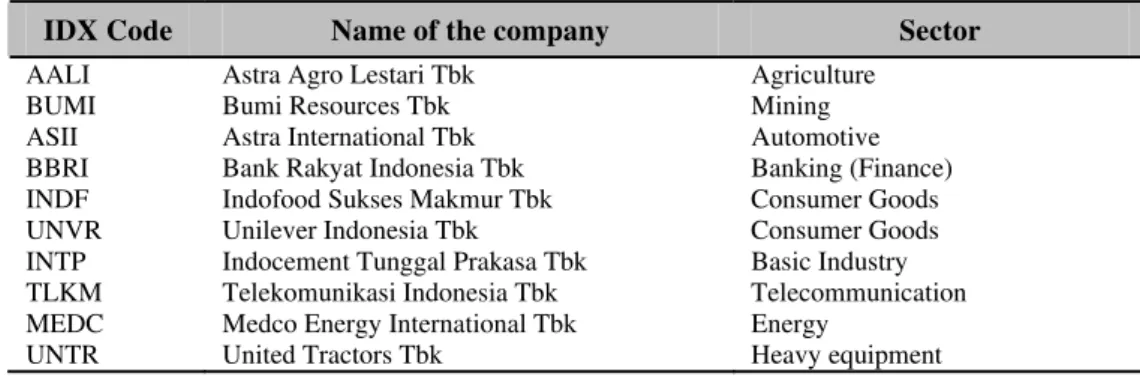
The first step that should be done is selecting the stocks to form portfolios. The Stocks that will be picked only 10 stocks which are always included in LQ 45 index which diversified among sectors namely telecommunication, mining/energy, agriculture, consumer goods, automotive, banking (finance), basic industry and heavy equipment.
Table 1 List of the 10 Stocks
IDX Code Name of the company Sector
AALI Astra Agro Lestari Tbk Agriculture BUMI Bumi Resources Tbk Mining ASII Astra International Tbk Automotive BBRI Bank Rakyat Indonesia Tbk Banking (Finance) INDF Indofood Sukses Makmur Tbk Consumer Goods UNVR Unilever Indonesia Tbk Consumer Goods INTP Indocement Tunggal Prakasa Tbk Basic Industry
TLKM Telekomunikasi Indonesia Tbk Telecommunication MEDC Medco Energy International Tbk Energy
UNTR United Tractors Tbk Heavy equipment
Portfolio Optimization
To determine an optimal portfolio there are several computation will be faced. At first, computation of expected return (mean) and risk (variance) of the 10 stocks and Index (JCI) to form Expected return (mean) and risk (variance) of portfolio. (Reilly & Brown, 2006)
Expected Return from an investment is defined as:
Where is the possible return of asset i and is the probability return. This equation to calculate the expected return of each asset in the portfolio
The formula of variance is as follows:
The larger the variance for an expected return, the larger the dispersion of expected returns and the greater the risk of the investment.
The next step is to compute the Expected return, Covariance and standard deviation of a portfolio
The expected return for a portfolio can be defined by this computation:
Where is the weight of an individual asset in the portfolio, and is the expected return for asset i. In order to find portfolio standard deviation ( portfolio), it is important to calculate the covariance
between assets first. Covariance is the degree of measurement to which two variables move together relative to their individual means value. A negative covariance shows that the rates of return for two assets tend to move in different direction while positive covariance shows that the rates of returns tend to move in the same direction. A value of zero indicates that the rates of return for two assets have no linear relationship. The formula of covariance of rates of return is defined as follow:
After covariance has been computed, the standard deviation can be calculated using this following formula:
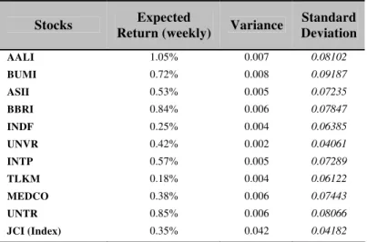
Where is the standard deviation of portfolio, it covers not only the variances of the individual assets but also the covariance between all pairs of individual assets in the portfolio. An optimum portfolio should have smaller standard deviation than individual asset’s standard deviation. Following is the result of computation of 10 stocks Expected Return, Variance and Standard Deviation:
Table 2 The Expected Return, Variance and Standard Deviation of 10 stocks
Stocks Expected
Return (weekly) Variance
Standard Deviation
AALI 1.05% 0.007 0.08102
BUMI 0.72% 0.008 0.09187
ASII 0.53% 0.005 0.07235
BBRI 0.84% 0.006 0.07847
INDF 0.25% 0.004 0.06385
UNVR 0.42% 0.002 0.04061
INTP 0.57% 0.005 0.07289
TLKM 0.18% 0.004 0.06122
MEDCO 0.38% 0.006 0.07443
UNTR 0.85% 0.006 0.08066
JCI (Index) 0.35% 0.042 0.04182
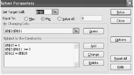
Figure 1 Solver for Optimization Portfolio
Mean-Variance formula is to obtain the expected return, variance and standard deviation of portfolio. Linear programming by solver excel is used to find each weight of stocks in one portfolio. Furthermore, it will be explained about the solver. From the figure 1, H8 is the portfolio variance, B2-B11 is the weight of each stock in the portfolio, B12 is the sum of the weight, and D12 is the expected return of the portfolio. Figure 1 shows set target cell is the objective of the solver ($H$8) which in this case is to minimize the variance of a portfolio. Changing cells refer to weight of the stocks in a portfolio ($B$2:$B$11). The sum of the weights will be constrained to 1 ($B$12 =1) and it means that each weight of stocks has to be zero or more ($B$2:$B$11 >= 0). The weights of stocks can change depend on the expected return that been set ($D$12 = $B$18).
From this computation, 10 sets of optimum portfolio can be obtained by changing the expected return and the following is the result of computation of 10 sets of optimum portfolios:
Table 3 10 Sets of Optimum Portfolio
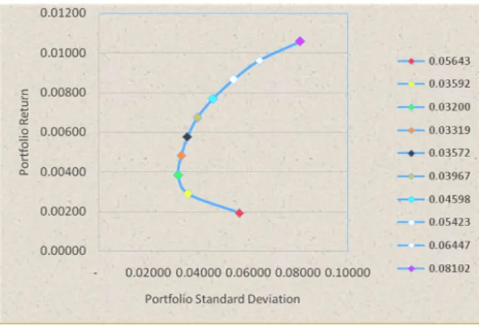
Portfolio Portfolio Return
Portfolio Standard Deviation
Portfolio A (red) 0.192% 0.05643
Portfolio B (yellow) 0.288% 0.03592
Portfolio C (Green) 0.385% 0.03200
Portfolio D (Orange) 0.481% 0.03319
Portfolio E (Black) 0.577% 0.03572
Portfolio F (Brown) 0.673% 0.03967
Portfolio G (Blue) 0.769% 0.04598
Portfolio H (White) 0.865% 0.05423
Portfolio I (Pink) 0.962% 0.06447
Portfolio J (Purple) 1.058% 0.08102
By this set of portfolios, the efficient frontier also can be curved as follow:
This efficient frontier signifies that set of portfolios which has the maximum rate of return for every given level of risk. From the above curve, it can be noticed clearly that Portfolio A, B, C are not an optimum portfolio because those portfolios give low level of return with high level of risk compare to other portfolios. In order to determine which portfolios is the optimum one, this study will use Sharpe formula.
The following is the formula of Sharpe:
Where is the average rate of return for portfolio i during given level of time, is the average rate of return on risk-free asset during given level of time and is the standard deviation of the portfolio.
Following is the result of computation using Sharpe’s evaluation:
Table 4 Sharpe’s Evaluation Stock Portfolio
Portfolio Portfolio
Return
Portfolio Standard
Deviation Sharpe
Portfolio A 0.192% 0.05643 0.002678
Portfolio B 0.288% 0.03592 0.030977
Portfolio C 0.385% 0.03200 0.064814
Portfolio D 0.481% 0.03319 0.091477
Portfolio E 0.577% 0.03572 0.111915
Portfolio F 0.673% 0.03967 0.125004
Portfolio G 0.769% 0.04598 0.128749
Portfolio H 0.865% 0.05423 0.126911
Portfolio I 0.962% 0.06447 0.121657
Portfolio J 1.058% 0.08102 0.108676
is the portfolio G. The problem is to determine the composition of each stock (weights) in that portfolio. To solve this problem, solver excel can be used to determine weights of each stock in the portfolio. The composition of each stock in that portfolio could be delivered from the solver (excel) computation.
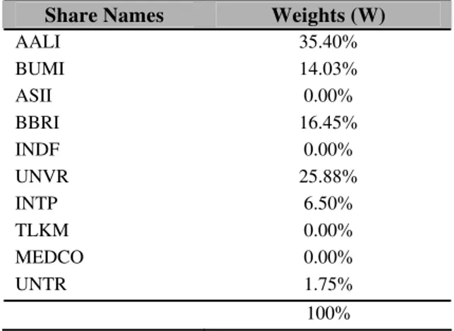
From the computation using solver above, the weights of each stock on the portfolio G are as follows:
Table 5 Composition (Weight) of Each Stock in Portfolio G
Share Names Weights (W)
AALI 35.40%
BUMI 14.03%
ASII 0.00%
BBRI 16.45%
INDF 0.00%
UNVR 25.88%
INTP 6.50%
TLKM 0.00%
MEDCO 0.00%
UNTR 1.75%
100%
It can be noted from the table 5 due to the optimization, there are some stocks have 0% of weight which means they have been excluded from the portfolio. The Stocks are ASII, INDF, TLKM and MEDC. Therefore, the stocks in the portfolio have been decreased to only 6 stocks.
Evaluation Performance
The next stage, this paper will evaluate the performance of the Portfolio G by using Sharpe, Treynor and and Jensen to ensure that the portfolio gives a superior return for a given level of risk compare to the market return.
Sharpe’s Evaluation:
From the computation of Sharpe’s evaluation, the results show that Sportfolio (0.128749) has
higher value than Smarket (0.04137251). It indicates that portfolio has exceeded the market.
Treynor’s Evaluation:
Where is the average rate of return for portfolio i during a given period of time, is the average rate of return of risk-free during a given period of time and is the Beta of portfolio.
From the computation, the result shows that Tportfolio has higher value (0.007507) than Tmarket (0.00173). It indicates that Portfolio has exceeded the market return.
Jensen’s evaluation:
Where = realized rate of return on a portfolio during a specified period of time, is the rate of return of risk free rate during a specified period of time, is the risk premium during specified period of time and is a random error term.
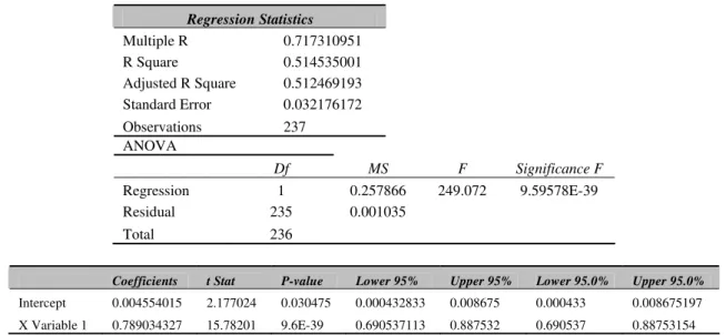
From the equation, the signifies if the portfolio is superior or inferior in stock selection and/or market timing. If the is positive, the portfolio is superior. In contrast, if the has negative value means that it is an inferior portfolio which means that returns of portfolio consistently fall short of expectations giving consistently negative residuals. Following is the result of Jensen computation on portfolio G:
Table 6 Jensen Measurement of a Portfolio
Regression Statistics
Multiple R 0.717310951 R Square 0.514535001 Adjusted R Square 0.512469193 Standard Error 0.032176172 Observations 237 ANOVA
Df MS F Significance F
Regression 1 0.257866 249.072 9.59578E-39 Residual 235 0.001035 Total 236
Coefficients t Stat P-value Lower 95% Upper 95% Lower 95.0% Upper 95.0%
Intercept 0.004554015 2.177024 0.030475 0.000432833 0.008675 0.000433 0.008675197 X Variable 1 0.789034327 15.78201 9.6E-39 0.690537113 0.887532 0.690537 0.88753154
The results show that portfolio is superior because the = + 0.004554015.
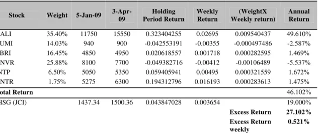
Optimum Portfolio for Forward Return
Table 7 Portfolio G for Forward Return
Stock Weight 5-Jan-09
3-Apr-09
Holding Period Return
Weekly Return
(WeightX Weekly return)
Annual Return
AALI 35.40% 11750 15550 0.323404255 0.02695 0.009540437 49.610% BUMI 14.03% 940 900 -0.042553191 -0.00355 -0.000497486 -2.587% BBRI 16.45% 4850 4950 0.020618557 0.001718 0.000282595 1.469% UNVR 25.88% 8100 7700 -0.049382716 -0.00412 -0.00106489 -5.537% INTP 6.50% 5050 5350 0.059405941 0.00495 0.000321559 1.672% UNTR 1.75% 5275 6300 0.194312796 0.016193 0.000283613 1.475%
Total Return 46.102%
IHSG (JCI) 1437.34 1500.36 0.043847028 0.003654 19.000%
Excess Return 27.102%
Excess Return
weekly
0.521%
Table 7 indicates that after 3 months return of portfolio exceeds the return of market by 27.10% annually or 0.52% weekly. Nonetheless, the computation of return do not consider about how much fund will be allocated into the portfolio since the study consider only to show how the portfolio return exceeds the market return. To evaluate whether it exceeds the market return, this paper uses some measurements such as Sharpe and Treynor
Table 8 Treynor and Sharpe Performance Evaluation
Weekly Annually
T Market 0.002212 0.115003789 T Portfolio 0.009413 0.489489278
S Market 0.052887 2.750130062 S Portfolio 0.161465 8.396189926
From table 8, it is clearly shown that Portfolio performance exceeds the market performance weekly and annually whether using Treynor or Sharpe measurement.
CONCLUSION
based on historical data series (5 years). However, in the real world there are more factors can affect the forward return such as market risk (interest rate risk, foreign exchange risk, and political risk). The author expectation’s that the further research can be more completed and sophisticated.
REFERENCES
Brealey, R. A., Myers, S. C., and Marcus, A. J. (2007). Fundamentals of corporate finance, New York: McGraw-Hill/Irwin.
Hull, J. (1995). Introduction to futures and options markets, Prentice Hall.
Indonesia Stock Exchange. (2008). Retrieved 2nd April 2010 from http://www.idx.co.id.
Konno, H. and Yamazaki, H. (1991). Mean-absolute deviation portfolio optimization model and its application to Tokyo stock market. Management Science, 37 (5), 519. Retrieved 30th March 2010 from
http://proquest.umi.com/pqdweb?index=0&did=106523&SrchMode=1&sid=1&Fmt=6&VInst =PROD&VType=PQD&RQT=309&VName=PQD&TS=1272531141&clientId=68814.
Lintner, J. (1965). The valuation of risky assets and the selection of risky investments in stock portfolios and capital budgets. Rev. Econ. Statist. 47.
Markowitz, H. (1959). Portfolio selection: Efficient diversification of investments, New York: John Wiley & Sons.
Mossin, J. (1966). Equilibrium in capital asset markets. Econometrica. 34.
Mossin, J. (1968). Optimal multiperiod portfolio policies. J.Business. 41.
Reilly, F. K., and Brown, K. C. (2006). Investment analysis and portfolio management, 8 ed.,USA: Thomson South-Western.
Sadewa, P. Y. (2009). Kredibilitas bursa saham perlu ditingkatkan. Danareksa Research Institute. Retrieved 2nd April 2009 from http://www.danareksa-research.com/economy/media-newspaper/242-kredibilitas-bursa-saham-perlu-ditingkatkan.
Sharpe, W. F. (1964). Capital asset prices: A theory of market equilibrium under conditions of risk. J. Financial, 19, 425-442.
Swisher, P., and Kasten G. W. (2005). Post-modern portfolio. FPA Journal. Retrieved 5th April 2010 from
http://www.fcva.net/Documents%20and%20Files/Post-Modern%20Portfolio%20Theory.pdf.