1 | P a g e
A Work Project, presented as part of the requirements for the Award of a Masters Degree in Economics / Finance / Management from the NOVA – School of Business and Economics.
RISK PARITY: “TRUE” VERSUS “NAÏVE” APPROACH
Gonçalo Filipe Abreu Alves
Student Number 495
A Project carried out on the Finance course, under the supervision of:
Afonso Fuzeta da Ponte Eça
2 | P a g e Abstract
Risk Parity: “True” vs “Naïve” Approach
This paper studies the performance of two different Risk Parity strategies, one from
Maillard (2008) and a “naïve” that was already used by market practitioners, against traditional strategies. The tests will compare different regions (US, UK, Germany and
Japan) since 1991 to 2013, and will use different ways of volatility. The main findings
are that Risk Parity outperforms any traditional strategy, and the “true” (by Maillard)
has considerable better results than the “naïve” when using historical volatility, while using EWMA there are significant differences.
3 | P a g e Index
1. Introduction
2. Literature Review
3. Methodology and Data
4. Results
a. Case 1
b. Case 2
c. Case 3
5. Conclusion
6. Bibliography
Annexes
4
5
8
11
12
14
18
22
24
4 | P a g e
1. Introduction
This paper will study the performance of portfolio strategy of Risk Parity. This strategy
takes a different approach when constructing a portfolio, we have some strategies that
are naïve, such as an equally-weighted (where all assets have the same weight, creating
“diversity”), a standard 60/40, allocating 60% of the capital on stocks and 40% on
bonds, having a defensive position; and we have others more complex such as a
minimum variance or Markowitz theory, where the objective is to maximize the Sharpe
ratio. Most of these schemes focus on maximizing the returns or have a simple asset
allocation which would provide high returns based on historical performances, except
for the minimum variance portfolio, which minimizes the volatility, but, nevertheless,
does not focus on the risk. What Risk Parity does is to equalize the risk contribution of
the assets, instead of the capital invested on assets. The marginal risk contribution is
simply the additional risk the portfolio would have if we would increase our position on
one asset by a small amount. This way, the strategy guarantees that every single asset
contributes with the same amount of risk to the overall portfolio’s risk. There are
several disadvantages of the previous mentioned strategies, which creates the
opportunity for other to arise. And that is how the Risk Parity idea surged. First, a more
naïve idea to calculate the weights for the assets, and later Maillard (2008) theorized the
problem and created a method to calculate the weights for the Risk Parity strategy
taking into account the covariance of the assets. With the mathematical theory
explaining the strategy it gained a lot of strength with various investigators backing it
up and even adding other features to the original one. What is interesting is that there
are several papers around the theme, some defending the theory, others creating more
5 | P a g e performance would outperform traditional ones, and there are some saying that there is
no evidence that Risk Parity is better than any of the existing ones. What will be done in
this paper first is to test the performance of Risk Parity strategies (naïve and the one
presented by Maillard) against traditional ones, analyze the results and compare them
with current literature. In a second part, there is going to be a performance test with
assets outside of USA and check if the results still hold; then, in the third part will be
dedicated to the estimation of the covariance matrix, changing the estimation method,
moving from historical data to EWMA mode. The fourth section will be dedicated to
the estimation of the covariance matrix, changing the estimation method, moving from
historical data to EWMA model.
This paper introduces to the current literature the testing of the Risk Parity strategies
outside USA and across world regions, since there is an extensive literature on US,
there is little information on the performance of the strategy outside, and none when
taking into account USA, Europe and Asia. Besides that, by using different methods of
calculating volatility gives a more robust results, widening the range of the tests. By
confronting the naïve strategy with the real Risk Parity strategy, we want to see if the
real RP outperforms and if it is worth the computational burden that the real RP
requires.
2. Literature Review
The first paper that is very important to this subject is the one by Maillard, Roncalli,
Teiletche (2010) because it is where the literature about risk parity started. It explains
6 | P a g e traditional strategies were questionable and the recent crisis showed their weaknesses.
The work focuses on the performance of the equally-weighted (EW) and
minimum-variance (MV) and how risk parity relate to them. The simple definition for risk parity
would be calculating a minimum-variance portfolio while applying an equally-weighted
filter, this would overcome the weaknesses of the minimum-variance that relies a lot on
the correlations between assets which can easily change in a matter of days (during a
critical time) and it can have huge impact on the performance. Risk parity, or
equally-weighted risk contribution (ERC) as it is named on this paper, has the specification of
maintaining the risk contribution of any asset in a portfolio equal. This way, changes on
any asset performance would have an equal impact on the portfolio. Comparing the
three strategies (MV, ERC and EW), the following relation is derived:
(1)
With this paper, many others appeared, Bruder and Roncalli (2013) extended the theory
to a more generalized, by giving the possibility of budgeting assets, instead of giving
them an equal budget like equally-weighted risk contribution strategy, which gives
more control over the portfolio and is especially interesting for strategic asset allocation.
Roncalli (2013) used the risk parity strategy to make it an active strategy, where the
investor could have an impact on the performance, by including expected returns.
Having a different risk measure (generalized standard deviation which incorporates
Gaussian value-at-risk and expected shortfall), this means that risk contribution has two
different fragments: performance contribution and volatility contribution. This is a very
interesting strategy because it allows to use knowledge to construct the portfolio and
7 | P a g e Another spin-off of the ERC is the tail risk parity, which focus on the prevention of the
worst scenarios. Alankar, DePalma, Scholes (2012) took into account the biggest fear of
investors (a big crisis) and proposed a strategy that would avoid those events depending
on the level of protection the investor would want. This strategy is much cheaper than
using market products to hedge the position while still yielding a high Sharpe ratio. The
objective is to minimize the cost dead-weight adjustments, which are very common and
are the cause of the bad performance of the portfolios during those negative peaks.
Although the work of Maillard is innovator, there are some criticism regarding the
theoretical support for that strategy. This is what Asness, Frazzini, Pedersen (2012) do
in their paper, finding evidence and explanation for the risk parity existence. Using the
example of a person that wants to yield a higher return than the market portfolio, that
person would invest more in risky assets, but if by any chance he cannot or does not
want to use leverage, the portfolio held would consist in all capital invested in stocks.
This leads to a problem if there is a large number of investors with the same restrictions
(which it happens) because it would overprice the stocks. When this happens, the
market portfolio is no longer the tangency portfolio, creating a gap between them. The
way to find an equilibrium is due to the underpricing of the safer assets, which yield
much higher risk-adjusted returns, and that is why risk parity strategies tend to
overweight safer assets.
In the last article, Anderson, Bianchi, Goldberg (2011) test the performance of the risk
parity strategies since 1926. The reason this paper is important is because in order to
replicate the strategy there are some problems regarding proxies to replace the actual
variables to be used, as much as the transaction costs, and this was not taken into
8 | P a g e separately gives different results, sometimes even risk parity strategy losing to
traditional strategies.
3. Methodology and Data
The data gathered for this work are the daily prices of future contracts of stock indexes
and government bonds from the United States of America, Japan, Germany and United
Kingdom. For further notice, the abbreviations used for tables and figures are described
in table 4.
The first step was to create the daily returns by taking the logarithms. Also, we
consider the monthly returns for the same data. Then we specify the portfolio
strategies, in this case it will be the equally-weighted (also known as EW or “1/n”), the traditional 60/40 (allocating 60% of the capital in stocks and 40% in bonds) and the
Risk Parity. The first two portfolios are simply calculated by taking the weights (that are
constant) and multiply by the returns, while for Risk Parity it is needed to calculate the
weights before.
In this paper the Risk Parity strategies will be rebalanced every day and every month.
For the monthly portfolios, the first day of every month, the weights for the strategy will
be different taking into account the previous performance. The weights for this strategy
will be calculated in a naïve way, meaning that they will be proportional to their
volatility, and also as Maillard (2008), taking into account the covariance between
9 | P a g e
∑
(2)
While for the “true” Risk Parity we have that the weights must be such that their
Marginal Risk Contribution is equal, so we have that the MRC to be:
( ) ( ) (3)
With to be the vector of weights and the covariance matrix. So the weights can be
calculated by using the formula:
(∑ )
∑ (∑ )
(4)
With to be the correlation vector. It is clear that there is a substantial difference
between the two methods, with this last one including the weights in order to calculate
the weights, meaning that the solution is endogenous. In order to solve the problem, we
have to create an algorithm, and the one that Maillard presents is the following:
( )
(5)
Where:
( ) ∑
∑ ( ( ) ( ) ) (6)
Which means that the function has the objective to minimize the difference of Marginal
Risk Contributions between the assets. These methods carry different workloads, the
naïve one can be calculated manually while the other requires estimation of a
covariance matrix and also heavy computing capabilities when dealing with large data.
In this paper, the variance and covariance matrix will be calculated with two different
10 | P a g e (EWMA). The first one gathers data from a determined number of periods and uses
them to generate a forecast, giving all the periods the same importance, it is the basic
variance. The EWMA differs from the SMA because it uses the historical data with
different weights for the periods, giving more relevance for those who are closer and
less to those which are further.
When assuming the sample mean ̅ is 0 and that infinite amounts of data are available
we have variance as follows:
∑( )
(7)
Where the λ (lambda) is the decaying factor. The smaller the lambda, the quicker the weight decays. One consequence of assuming the sample mean is 0 is that it allows the
use of the recursive feature of the EWMA since the forecast depends on the value of the
previous period, so it is possible to create a dynamic model for forecasting as follows:
( ) (8)
It is more obvious in this equation that the value of the decay factor plays an important
role on predicting variances, so, using a small lambda can cause problems because
important data may be “forgot” as well as using a very high one, because it approaches to the SMA. According to RiskMetrics, the optimal decaying factor values for a one-day
forecast is 0.94 and for a one month is 0.97, and these values will be used. Another
important thing that this dynamic model creates is the ability to generate new forecast
recursively, saving time which is a burden when dealing with large amounts of data.
11 | P a g e
( ) (9)
After some calculations, the volatilities and covariances of the EWMA showed some
problems, mainly due to the first value of the series estimated. In fact, the value was far
away from the realistic ones, and due to the recursive formula for the forecasts, this
problem would drag for some quite time in the series until the effect would wore of and
dissipate. So, in order to avoid this problem and not losing data, the first value of the
series has been replaced for the simple variance of the entire series. This results in a
more realistic value and makes the series to converge to its actual values much faster.
Having the portfolios calculated, to compare the performances, will be calculated some
descriptive statistics such as average annual return, annual volatility, Sharpe ratio,
kurtosis, skew and quartile distribution. It is expected that both Risk Parity strategies
outperform the others in terms of volatility and Sharpe ratio, and among the Risk Parity,
the “true” should have lower volatility.
4. Results
In this section will be analyzed the outputs of the tests through the descriptive analyses.
In a first moment there will be the comparison of the different portfolio strategies, in a
monthly basis. This part will have a simple moving average method for the calculation
of volatility. After the first part there is going to be an evaluation of the risk parity
strategies: the “naïve” against the “true”, in a portfolio with all the countries included (8
assets) and with the benchmark of the equally weighted. After that, there is going to be
a discussion whether if it is optimal to create a portfolio with all the assets or if it is
12 | P a g e Parity is capable of increasing its performance with a large number of assets (diversity).
The next part will be checking if the results still hold when moving from a SMA
approach to a EWMA.
a. Case 1
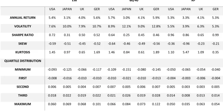
This section is dedicated to the analysis of the back tests. In a first part there will be the
comparison between the traditional strategies against the Risk Parity in a two asset
scenario, this means that four portfolios are generated, one per country, having an asset
based on that country’s stocks and bonds. The monthly portfolios’ descriptive statistics are in Table 1 and show the expected results of a lower volatility and a higher Sharpe
ratio as expected.
Table 1
EW 60/40 RP
USA JAPAN UK GER USA JAPAN UK GER USA JAPAN UK GER
ANNUAL RETURN 5.4% 3.1% 4.0% 5.6% 5.7% 3.0% 4.1% 5.9% 5.3% 3.3% 4.1% 5.3%
VOLATILITY 7.6% 10.0% 7.9% 10.7% 8.9% 12.1% 9.0% 12.8% 5.5% 3.9% 6.3% 5.3%
SHARPE RATIO 0.72 0.31 0.50 0.52 0.64 0.25 0.45 0.46 0.96 0.86 0.65 0.99
SKEW -0.59 -0.51 -0.45 -0.52 -0.64 -0.46 -0.49 -0.56 -0.36 -0.96 -0.23 -0.21
KURTOSIS 1.45 0.97 0.65 1.69 1.46 0.84 0.61 1.89 1.10 5.47 1.09 0.35
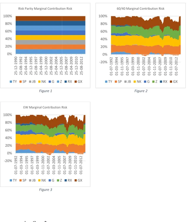
To further analyze the strategies in a risk management optic, we can check the marginal
risk contributions that are in Figures 1 to 3. The Risk Parity graph shows equality
between all the assets, as expected by the definition, which does not mean it is related to
the weights allocated. In Figure 1 it is plotted the weights for the Risk Parity and it is
obvious that it is dominated by the risk-free assets, and this can be explained in different
13 | P a g e the asset based on stock market, so it is logical that the weights must higher on bonds to
compensate and equalize the risk. Other explanation for this fact is that, contrary to
what traditional portfolios “sell”, the amount of capital invested in a portfolio’s asset isn’t directly correlated to the amount of risk that person wants to assume, so this comes
to show that those are two different concepts. The traditional strategies are very similar
due to its composition, so they share similar results. Although is most of the cases one
of them yields the highest annual return, the portfolios fail when analyzing the
volatilities, where it sometimes double the ones from the Risk Parity. This is rather
important for the case of the low risk profile, where investors want to assume a very low
level of risk and end up yielding one of the highest volatilities. When checking the
marginal risk contributions the results are very different from the Risk Parity. The
figures 1 to 3 show that the portfolios are dominated by the risky asset, having values
near 90% but reaching over 100% in some cases. This shows how bad the
diversification of risk in these portfolios is. Another interesting fact that can be seen in
the table is the negative peaks that the portfolios have: the traditional portfolios can
have a negative return of 15% a year, while the Risk Parity is much more protected to
spikes, either negative or positive.
This test has a unique specification that will not be used in the next sections, that is the
fact that being using portfolios it is not possible to test the risk parity “true” and “naïve”
since the “true” one has a unique solution for the case of two assets, which is the
“naïve” solution. This happens because, as Maillard shown, the solution does not
depend on asset correlation, so it is easy to calculate without recurring to optimization
14 | P a g e This test concludes what the current literature says, the superiority of the Risk Parity in
terms of the risk and Sharpe ratio. What is important for this paper is to study the Risk
Parity itself, rather than compare it with other strategies.
Figure 1 Figure 2
Figure 3
b. Case 2
The next part is solely dedicated to study the different Risk Parity strategies, that is, the
“true” Risk Parity from the “naïve”. This is important to study because Risk Parity has 0%
20% 40% 60% 80% 100%
25-12-1990 25-08-1992 25-04-1994 25-12-1995 25-08-1997 25-04-1999 25-12-2000 25-08-2002 25-04-2004 25-12-2005 25-08-2007 25-04-2009 25-12-2010 25-08-2012
Risk Parity Marginal Contribution Risk
TY SP JB NK G Z RX GX
-20% 0% 20% 40% 60% 80% 100%
01-07-1992 01-03-1994 01-11-1995 01
-07
-19
97
01-03-1999 01-11-2000 01-07-2002 01-03-2004 01-11-2005 01-07-2007 01
-03
-20
09
01-11-2010 01-07-2012
60/40 Marginal Contribution Risk
TY SP JB NK G Z RX GX
-20% 0% 20% 40% 60% 80% 100%
01-07-1992 01-03-1994 01-11-1995 01-07-1997 01-03-1999 01-11-2000 01-07-2002 01-03-2004 01-11-2005 01-07-2007 01-03-2009 01-11-2010 01-07-2012
EW Marginal Contribution Risk
15 | P a g e
been used for some quite time but in the “naïve” form instead of the one proposed by
Maillard. The “naïve” form, as explained before, just takes the weights as proportion of the asset’s volatility compared to the portfolio’s. So, the test for the Risk Parity strategy will be as follow: testing in a general case for one large portfolio with eight assets, this
means four risk-free assets and four risky assets, being the most complex to calculate
with the current data. It is important to remind that the computational burden for the
“true” form is very heavy, for the eight asset portfolio it is needed to calculate thirty six variances and covariances and also requires an optimization for every date.
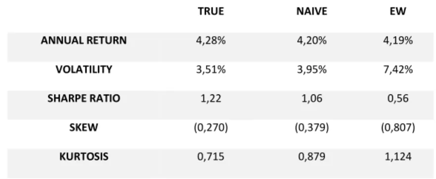
The results will also have the equally-weighted portfolio to be used as benchmark for
the traditional strategies. The results are shown in table 2 and it is interesting to see that
the annual return is very close but the volatility is higher on the naïve approach by near
half percent point. The Sharpe ratio is still higher on the true form, but the statistical
distribution is very similar.
Table 2
TRUE NAIVE EW
ANNUAL RETURN 4,28% 4,20% 4,19%
VOLATILITY 3,51% 3,95% 7,42%
SHARPE RATIO 1,22 1,06 0,56
SKEW (0,270) (0,379) (0,807)
KURTOSIS 0,715 0,879 1,124
It is interesting to compare both the weights and marginal risk contributions, presented
in figures 4. At a glance, looking at the weights they are similar, giving more weight to
the assets with less volatility, and less weight to the one with higher risk, but we see that
16 | P a g e
to the plots of the marginal risk contributions we see a very different picture: the “true”
portfolio has a constant MRC of 12.5% across time while the other is rather chaotic,
while in some periods there seems to be some kind of balance along all the assets
(which it does not really happen), there is actually some spikes in the graph where some
assets contribution are reduce to zero or even be negative for few moments. This is
critical, especially when an investor bets on a strategy that has the objective of
managing risk and wants to control it. So having those few moments where the risk
shoots to the roof is a huge flaw to the strategy, and it should be also a strength of the
Risk Parity to be reliable during dangerous times. When comparing to the
equally-weighted portfolio, the highlight is the volatility that is more than the double of the
other two strategies, causing a very low Sharpe ratio.
This test shows a superior portfolio but it is interesting to continuing to test for more
reliable results, so, in order to get more results to compare and judge if there is really a
difference between the two strategies, I am going to make a battery of test for all
possible combinations of portfolios among the countries. The objective is to have more
than “one path”, which is one of the main criticism made to Risk Parity, because it hasn’t been used by investors for an enough time, so the empirical results that exist are
very few and are based on the principles. By doing this, I pretend to see if the previous
result occurred due to a specific asset that could have a great impact on the portfolio,
and if an investor could select its portfolio, he could drop the position on that specific
asset and achieve better returns.
The results shown in tables 7 to 16 of the Annexes, are in line with the previous one, in
terms of volatility and Sharpe ratio, the “true” Risk Parity has better results, and these
17 | P a g e almost every test. Also, the fact that we are using different number of assets it is
possible to see that, from table 1 (the specific case of portfolios with two assets), table 2
and the ones from the annexes, we see that there is increased Sharpe ratio as we add up
more assets. This could mean that the risk parity performs better with more assets due to
its diversification feature, which is a strength that makes the strategy very powerful.
Another relevant fact that should be debated is the weight of the risk-free assets on the
portfolio. We see that in both strategies they have a high percentage of the portfolio
composition and it does not change abruptly, instead, when there is some turbulence
there is actually a move from one country to other risk-free. This happens because risky
assets are very volatile and it is very hard to match it, so there is a need of a large
quantity of low volatility assets. In a more theoretical explanation, using the work of
Asness, Frazzini, Pedersen (2012), this happens because the risky assets are
over-valued, the amount of returns it offers does not compensate the risk it yields, and the
opposite happens, the risk-free assets are under-valued, meaning they are offering much
higher returns than they should. This happens because of the amount of demand for
risky assets that traditional assets require, and also, for the different risk profiles, if one
would look to the risk contributions instead of capital allocated, the weights would be
18 | P a g e F ig u re 4 – W ei gh ts an d m arg ina l risk co ntri bu tio ns fo r th e “t ru e”, “ na ïve” a n d eq u a lly -w ei g h te d p o rt fo lio s w ith h ist o rica l v o la ti lity .
0% 10% 20% 30% 40% 50% 60% 70% 80% 90%
100% 30-11-1991 30-11-1993 30-11-1995 30-11-1997 30-11-1999 30-11-2001 30-11-2003 30-11-2005 30-11-2007 30-11-2009 30-11-2011 30-11-2013 "T rue " R isk P ar ity we ig ht s TY SP JB NK g z rx gx
0% 10% 20% 30% 40% 50% 60% 70% 80% 90%
100% 30-11-1991 30-11-1993 30-11-1995 30-11-1997 30-11-1999 30-11-2001 30-11-2003 30-11-2005 30-11-2007 30-11-2009 30-11-2011 30-11-2013 "T rue " R isk P ar ity m ar g ina l c o nt ribu tio n risk TY SP JB NK g z rx gx
0% 10% 20% 30% 40% 50% 60% 70% 80% 90%
100% 30-11-1991 30-11-1993 30-11-1995 30-11-1997 30-11-1999 30-11-2001 30-11-2003 30-11-2005 30-11-2007 30-11-2009 30-11-2011 30-11-2013 "Na iv e " R isk P ar ity we ig ht s TY SP JB NK g z rx gx -20%
0% 20% 40% 60% 80%
100% 01-11-1991 01-11-1993 01-11-1995 01-11-1997 01-11-1999 01-11-2001 01-11-2003 01-11-2005 01-11-2007 01-11-2009 01-11-2011 01-11-2013 "Na iv e " R isk P ar ity m ar g ina l r isk c o nt ribu tio n TY SP JB NK g z rx gx
0% 10% 20% 30% 40% 50% 60% 70% 80% 90%
100% 30-11-1991 30-11-1993 30-11-1995 30-11-1997 30-11-1999 30-11-2001 30-11-2003 30-11-2005 30-11-2007 30-11-2009 30-11-2011 30-11-2013 E qu al ly -we ig ht e d we ig ht s TY SP JB NK g z rx gx -20%
0% 20% 40% 60% 80%
19 | P a g e
c. Case 3
To continue the journey to understand if Risk Parity is a strategy that is worth to be
invested continues but this time the test relies on the risk measure, the volatility, where
we jump from the simple moving average to the exponential weighted moving average.
The goal here is to understand if the method of calculating the volatilities influences the
results of the strategies. By using EWMA we are giving less relevance to more
distanced days, this could mean a faster reaction to the strategies to adapt for some
sudden events. It is also good to have more information on how the strategy performs
under different assumptions, since there is not much literature on the topic, testing under
new hypothesis adds value to the performance. For this test, it will be tested with a
portfolio with all assets, and the combination of the countries results will be displayed
on the annexes. The results are in table 3 and show that “true” Risk Parity has a higher Sharpe ratio, but this time there is a significant lower difference between both strategies,
Sharpe ratio is only 0.05 points higher, with annual returns being greater on the “naïve” and the volatility also being very close on both. When comparing to the previous tests,
using the historical volatility, that there is indeed a smaller Sharpe using EWMA for
both risk parity strategies and slightly higher for the equally-weighted portfolio.
Table 3
TRUE NAIVE EW
ANNUAL RETURN 3,94% 4,03% 4,21%
VOLATILITY 3,83% 4,11% 7,42%
SHARPE RATIO 1,03 0,98 0,57
SKEW (0,213) (0,278) (0,810)
20 | P a g e This may seem to have an impact on the strategy performance, so analyzing the
composition of the weights and marginal risk contribution may give a better insight. In
figure 5 we have charted the marginal risk contributions and weights. Checking the
marginal risk contributions first, the “true” strategy has equal values for all assets as
expected and for the “naïve” it is quite similar to the “true”, constant during time and quite balanced among the assets. It is actually better in terms of protection against
spikes, there is actually one small peak during the crisis of 2008. As for the weights it is
interesting to see that both graphs are identical regarding the distributions across assets,
with the “naïve” being more stable and constant and also the “true” reacts more abruptly than the other. The EWMA can be actually good when taking into account transaction
costs. While it yield lower Sharpe ratio, by keeping constant weights and marginal
contributions to risk among both strategies, the investor could be in a more comfortable
position knowing that this way the transaction costs would be much lower. Comparing
both “true” risk parity strategies, there is a big difference on how wildly it moves when
using the SMA and how steady it is on EWMA. The fact that the weights are much
stable in these tests show that there is a protection against crisis. This is what Ashwin
Alankar, Michael DePalma, Myron Scholes on their work on Tail Risk Parity proposed,
because during those crucial times the correlation between assets change so much, the
composition of the portfolios suffers drastic changes too to maintain the same level of
risk. And what happens is that usually in order to adapt to those changes, the investors
need more money to face transaction costs, and also, to try to minimize the losses
usually they opt to sell the most liquid assets first, which results in deadweight-loss. So,
in a way, when using EWMA to estimate volatility is actually applying a kind of Tail
21 | P a g e return by a small amount and the Sharpe ratio, but gains protection against low
probability events, which are the biggest fear of investors with low risk profile.
In the Annexes we can find the results of the tests of the combination of the different
countries and it follows the marks of the previous test: a smaller Sharpe ratio mainly
because of slightly higher volatility and in some cases smaller returns. Also, by seeing
the plots of the “naïve” strategy presented in figures 6 and 8, we see that the distribution of the weights assume an identical distribution of weights as the previous test, great
weight given to risk-free assets and in the particular case of the EWMA, more stable
through time. It is interesting the fact that in this case, the “naïve” risk parity graphs of the marginal risk contributions are very close to the “true” one. This might create a
relation between the method used to estimate volatility and the marginal risk
contributions, by weighting heavily the most recent events, the “naïve” strategy would
perform better in terms of stability. In terms of Sharpe ratio, it is still better to use the
simple moving average, but the difference is relatively small.
0% 10% 20% 30% 40% 50% 60% 70% 80% 90% 100%
01-11-91 01-10-93 01-09-95 01-08-97 01
-07
-99
01-06-01 01-05-03 01-04-05 01-03-07 01-02-09 01-01-11 01
-12
-12
"True" Weights (EWMA)
TY SP JB NK g z rx gx
0% 20% 40% 60% 80% 100%
01-11-91 01-10-93 01-09-95 01-08-97 01-07-99 01-06-01 01
-05
-03
01-04-05 01-03-07 01-02-09 01-01-11 01-12-12
"True" Risk Parity Marginal Risk Contribution (EWMA)
22 | P a g e
Figure 5 - Weights and marginal risk contributions for the “true”, “naïve” and equally-weighted portfolios with
EWMA volatility.
5. Conclusion
This paper had the goal to understand how the Risk Parity is being used by practitioners
and what are the main advantages of that compared to the traditional strategies, and
after seeing how well it does, the objective was to compare both Risk Parities strategies,
the ones most used by investors (“naïve” form) against the one Maillard created to truly
balance the risk among all the assets in a portfolio. After this, it was time to see if the
empirical results present were in fact able to be reproduced in the financial world, to see
the strategy in action, because there are exogenous factors such as the transaction costs
and the time discrepancy that make the investor’s work hard to put in practice and as
well as the burden one have to manage the portfolio with such technical requirements.
In the end, it was confirmed the hypothesis that the Risk Parity outperforms the
traditional strategies and also the “true” Risk Parity to yield better than the “naïve” in
the very different assumptions made: testing for different number of assets and the
calculation of the volatility. This strategy grants the highest Sharpe ratio among the
0% 10% 20% 30% 40% 50% 60% 70% 80% 90% 100%
01-11-1991 01-10-1993 01-09-1995 01-08-1997 01
-07
-19
99
01-06-2001 01-05-2003 01-04-2005 01-03-2007 01-02-2009 01-01-2011 01
-12
-20
12
"Naive" Weights (EWMA)
TY SP JB NK g z rx gx
0% 20% 40% 60% 80% 100%
01-11-1991 01-10-1993 01-09-1995 01-08-1997 01-07-1999 01-06-2001 01
-05
-20
03
01-04-2005 01-03-2007 01-02-2009 01-01-2011 01-12-2012
"Naive" Risk Parity Marginal Risk Contribution (EWMA)
23 | P a g e ones testes, and literature provides empirical evidence that it is better than any of the
traditional strategies and is very close to the minimum variance. The advantages of the
risk parity strategy can easily overcome the smaller Sharpe ratio, due to its properties of
equally-weighted risk contribution that grants the said high Sharpe ratio and takes into
account all assets, creating a balance between all of them, while the minimum variance
in order to maximize the Sharpe ratio can ignore some of the assets due to the
covariance and correlation between assets, which makes it more vulnerable to sudden
movements and crisis, which significantly change the correlations between assets, and
then the composition of the portfolio.
It is also important to underline that the “naïve” Risk Parity yield a high Sharpe ratio compared to the equally-weighted portfolio, used as benchmark for the traditional
strategies, and close to the “true” one. It can be considered as an alternative for investors that do not want to spend time in complicated calculations, but it would be
wise that when opting for this one, to use the EWMA or other similar methodology to
calculate volatility because it has a high impact on the performance of the portfolio:
while it may give a not so significant smaller Sharpe ratio, it provides a more stable
weights during time, and also does not wildly moves during crisis, which is a good
natural protection.
The conclusion is obvious, the “true” Risk Parity yield much better results than its
24 | P a g e 6. Bibliography:
Acemoglu, Daron. 2002. “Technical Change, Inequality, and the Labor Market.”
Journal of Economic Literature, 40(1): 7–72.
Sébastien Maillard, Thierry Roncalli, Jérôme Teïletche, Summer 2010, “The
Properties of Equally Weighted Risk Contribution Portfolios” The Journal of Portfolio Management, Vol. 36, No. 4: pp. 60-70.
Robert M. Anderson, Stephen W. Bianchi, Lisa R. Goldberg, November / December
2012, “Will My Risk Parity Outperform?” Financial Analysts Journal, Vol. 68, No. 6,
19 pages.
Thierry Roncalli, “Introducing Expected Returns into Risk Parity Portfolios: A New
Framework for Tactical and Strategic Asset Allocation” – working paper
Clifford S. Asness, Andrea Frazzini, Lasse H. Pedersen, 2012, “Leverage Aversion
and Risk Parity” Financial Analyst Journal, Volume 68, Number 1
Benjamin Bruder, Thierry Roncalli, January 2013, “Managing Risk Exposures using
the Risk Parity Approach” Research by Lyxor
Ashwin Alankar, Michael DePalma, Myron Scholes, 2012, “An Introduction to Tail
25 | P a g e Annexes
Table 4
Abbreviation Bloomberg Ticker Description
TY TY 1 US Treasury Yield
SP SP 1 Standard and Poor's Index
JB JB 1 Japanese Bonds
NK NK 1 Nikkei Index
G G 1 UK Government Yield
Z Z 1 FTSE Index
RX RX 1 Germany Government Yield
GX GX 1 Dax Index
Case 1
Table 5- Full descriptive statistics
EW 60/40 RP
USA JAPAN UK GER USA JAPAN UK GER USA JAPAN UK GER
ANNUAL RETURN 5.4% 3.1% 4.0% 5.6% 5.7% 3.0% 4.1% 5.9% 5.3% 3.3% 4.1% 5.3%
VOLATILITY 7.6% 10.0% 7.9% 10.7% 8.9% 12.1% 9.0% 12.8% 5.5% 3.9% 6.3% 5.3%
SHARPE RATIO 0.72 0.31 0.50 0.52 0.64 0.25 0.45 0.46 0.96 0.86 0.65 0.99
SKEW -0.59 -0.51 -0.45 -0.52 -0.64 -0.46 -0.49 -0.56 -0.36 -0.96 -0.23 -0.21
KURTOSIS 1.45 0.97 0.65 1.69 1.46 0.84 0.61 1.89 1.10 5.47 1.09 0.35
QUARTILE DISTRIBUTION
MINIMUM -0.093 -0.125 -0.066 -0.117 -0.109 -0.151 -0.080 -0.145 -0.050 -0.065 -0.054 -0.040
FIRST -0.008 -0.016 -0.010 -0.010 -0.010 -0.021 -0.010 -0.013 -0.004 -0.003 -0.006 -0.004
SECOND 0.006 0.005 0.004 0.007 0.007 0.005 0.006 0.007 0.005 0.003 0.003 0.005
THIRD 0.018 0.022 0.019 0.022 0.021 0.026 0.019 0.028 0.014 0.008 0.013 0.014
26 | P a g e
Case 2
Table 6- Full descriptive statistics
TRUE NAIVE EW
ANNUAL RETURN 4,28% 4,20% 4,19%
VOLATILITY 3,51% 3,95% 7,42%
SHARPE RATIO 1,22 1,06 0,56
SKEW (0,270) (0,379) (0,807)
KURTOSIS 0,715 0,879 1,124
By geography:
1. Two countries
Table 7- US and Germany
TRUE NAIVE EW
ANNUAL RETURN 5.24% 5.22% 5.51%
VOLATILITY 4.67% 4.74% 8.27%
SHARPE RATIO 1.122 1.102 0.666
SKEW (0.203) (0.270) (0.580)
KURTOSIS 0.942 0.857 1.233
Table 8- US and Japan
TRUE NAIVE EW
ANNUAL RETURN 3.86% 3.82% 3.76%
VOLATILITY 3.48% 3.75% 7.69%
SHARPE RATIO 1.109 1.020 0.489
SKEW (0.385) (0.390) (0.859)
KURTOSIS 1.936 1.604 1.912
Table 9- US and UK
TRUE NAIVE EW
ANNUAL RETURN 4.82% 4.72% 4.60%
VOLATILITY 5.13% 5.24% 7.29%
SHARPE RATIO 0.940 0.900 0.631
SKEW (0.271) (0.289) (0.538)
KURTOSIS 1.030 0.901 0.722
Table 10- Japan and Germany
TRUE NAIVE EW
ANNUAL RETURN 3.93% 3.93% 3.82%
VOLATILITY 3.39% 3.61% 8.83%
SHARPE RATIO 1.161 1.089 0.432
SKEW (0.024) (0.163) (0.690)
27 | P a g e Table 11- Japan and UK
TRUE NAIVE EW
ANNUAL RETURN 3.17% 3.36% 2.90%
VOLATILITY 2.93% 3.83% 7.60%
SHARPE RATIO 1.084 0.878 0.382
SKEW (0.301) (0.237) (0.766)
KURTOSIS 0.992 0.712 1.128
Table 12- UK and Germany
TRUE NAIVE EW
ANNUAL RETURN 4.75% 4.63% 4.66%
VOLATILITY 5.25% 5.30% 8.63%
SHARPE RATIO 0.905 0.874 0.540
SKEW (0.332) (0.356) (0.605)
KURTOSIS 0.586 0.546 0.827
2. Three countries
Table 13- US, Japan and Germany
TRUE NAIVE EW
ANNUAL RETURN 4.19% 4.23% 4.36%
VOLATILITY 3.38% 3.72% 7.79%
SHARPE RATIO 1.2407 1.1380 0.5596
SKEW (0.1418) (0.2797) (0.8131)
KURTOSIS 0.8936 0.9866 1.2870
Table 14- US, UK and Japan
TRUE NAIVE EW
ANNUAL RETURN 3.92% 3.88% 3.75%
VOLATILITY 3.49% 3.91% 7.07%
SHARPE RATIO 1.1220 0.9905 0.5309
SKEW (0.3429) (0.3583) (0.8604)
KURTOSIS 1.3382 1.1238 1.5757
Table 15- US, UK and Germany
TRUE NAÏVE EW
ANNUAL RETURN 4.96% 4.84% 4.92%
VOLATILITY 4.73% 4.87% 7.80%
SHARPE RATIO 1.0489 0.9939 0.6312
SKEW (0.2619) (0.3248) (0.6156)
KURTOSIS 0.6908 0.5928 0.8053
Table 16- Japan, UK and Germany
TRUE NAIVE EW
ANNUAL RETURN 3.97% 3.88% 3.79%
VOLATILITY 3.53% 3.94% 7.88%
SHARPE RATIO 1.1242 0.9850 0.4815
SKEW (0.0913) (0.2383) (0.7662)
28 | P a g e
Case 3
Table 17 - Full descriptive statistics
TRUE NAIVE EW
ANNUAL RETURN 3,94% 4,03% 4,21%
VOLATILITY 3,83% 4,11% 7,42%
SHARPE RATIO 1,03 0,98 0,57
SKEW (0,213) (0,278) (0,810)
KURTOSIS 0,306 0,463 1,128
By geography tables:
1. Two countries
Table 18- US and Germany
TRUE NAIVE EW
ANNUAL RETURN 5,01% 4,96% 5,51%
VOLATILITY 5,01% 4,99% 8,27%
SHARPE RATIO 1,001 0,995 0,666
SKEW (0,257) (0,267) (0,580)
KURTOSIS 0,617 0,673 1,233
Table 19- US and Japan
TRUE NAIVE EW
ANNUAL RETURN 3,85% 3,93% 3,76%
VOLATILITY 4,07% 4,12% 7,69%
SHARPE RATIO 0,946 0,953 0,489
SKEW (0,527) (0,468) (0,859)
KURTOSIS 1,931 1,886 1,912
Table 20- US and UK
TRUE NAIVE EW
ANNUAL RETURN 4,43% 4,41% 4,60%
VOLATILITY 5,51% 5,56% 7,29%
SHARPE RATIO 0,804 0,793 0,631
SKEW (0,347) (0,350) (0,538)
KURTOSIS 0,780 0,787 0,722
Table 21- Japan and German
TRUE NAIVE EW
ANNUAL RETURN 3,74% 3,75% 3,82%
VOLATILITY 3,87% 3,92% 8,83%
SHARPE RATIO 0,965 0,956 0,432
SKEW (0,320) (0,257) (0,690)
29 | P a g e Table 22- Japan and UK
TRUE NAIVE EW
ANNUAL RETURN 2,99% 3,19% 2,90%
VOLATILITY 3,02% 4,18% 7,60%
SHARPE RATIO 0,991 0,764 0,382
SKEW (0,256) (0,362) (0,766)
KURTOSIS 0,539 0,732 1,128
Table 23- UK and Germany
TRUE NAIVE EW
ANNUAL RETURN 4,21% 4,17% 4,66%
VOLATILITY 5,56% 5,55% 8,63%
SHARPE RATIO 0,758 0,752 0,540
SKEW (0,274) (0,288) (0,605)
KURTOSIS 0,235 0,251 0,827
Three countries
Table 24 – US, Japan and Germany
TRUE NAIVE EW
ANNUAL RETURN 4,28% 4,19% 4,36%
VOLATILITY 3,96% 4,04% 7,79%
SHARPE RATIO 1,0793 1,0366 0,5596
SKEW (0,3555) (0,3030) (0,8131)
KURTOSIS 0,8860 0,9062 1,2870
Table 25 – US, UK and Japan
TRUE NAIVE EW
ANNUAL RETURN 3,73% 3,82% 3,75%
VOLATILITY 4,10% 4,28% 7,07%
SHARPE RATIO 0,9106 0,8924 0,5309
SKEW (0,4320) (0,4030) (0,8604)
KURTOSIS 1,2241 1,1790 1,5757
Table 26 – US, UK and Germany
TRUE NAIVE EW
ANNUAL RETURN 4,58% 4,52% 4,92%
VOLATILITY 5,14% 5,16% 7,80%
SHARPE RATIO 0,8904 0,8754 0,6312
SKEW (0,2937) (0,3112) (0,6156)
KURTOSIS 0,4034 0,4145 0,8053
Table 27 – Japan, UK and Germany
TRUE NAIVE EW
ANNUAL RETURN 3,97% 3,88% 3,79%
VOLATILITY 3,53% 3,94% 7,88%
SHARPE RATIO 1,1242 0,9850 0,4815
SKEW (0,0913) (0,2383) (0,7662)
30 | P a g e By geography graphs:
Weights and marginal risk contributions two countries
0% 10% 20% 30% 40% 50% 60% 70% 80% 90% 100%
01-11-1991 01-10-1993 01-09-1995 01-08-1997 01-07-1999 01-06-2001 01
-05
-20
03
01-04-2005 01-03-2007 01-02-2009 01-01-2011 01-12-2012
"Naive" weights - US and Germany
TY SP RX GX
0% 10% 20% 30% 40% 50% 60% 70% 80% 90% 100%
01-11-1991 01-10-1993 01-09-1995 01-08-1997 01-07-1999 01-06-2001 01-05-2003 01-04-2005 01-03-2007 01-02-2009 01-01-2011 01-12-2012
"Naive" marginal risk contributions - US and Germany
TY SP RX GX
0% 10% 20% 30% 40% 50% 60% 70% 80% 90% 100%
01-11-1991 01-10-1993 01-09-1995 01-08-1997 01-07-1999 01-06-2001 01
-05
-20
03
01-04-2005 01-03-2007 01-02-2009 01-01-2011 01-12-2012
"Naive" weights - Japan and Germany
JB NK RX GX
0% 10% 20% 30% 40% 50% 60% 70% 80% 90% 100%
01-11-1991 01-10-1993 01-09-1995 01-08-1997 01-07-1999 01-06-2001 01-05-2003 01-04-2005 01-03-2007 01-02-2009 01-01-2011 01-12-2012
"Naive" marginal risk contributions - Japan and Germany
31 | P a g e
0% 10% 20% 30% 40% 50% 60% 70% 80% 90%
100% 01-11-1991 01-10-1993 01-09-1995 01-08-1997 01-07-1999 01-06-2001 01-05-2003 01-04-2005 01-03-2007 01-02-2009 01-01-2011 01-12-2012 "Na iv e " we ig ht s - UK an d G e rm an y G Z RX GX
0% 10% 20% 30% 40% 50% 60% 70% 80% 90%
100% 01-11-1991 01-10-1993 01-09-1995 01-08-1997 01-07-1999 01-06-2001 01-05-2003 01-04-2005 01-03-2007 01-02-2009 01-01-2011 01-12-2012 "Na iv e " m ar g ina l r isk c o nt ribu tio ns UK an d G e rm an y G Z RX GX
0% 10% 20% 30% 40% 50% 60% 70% 80% 90%
100% 01-11-1991 01-10-1993 01-09-1995 01-08-1997 01-07-1999 01-06-2001 01-05-2003 01-04-2005 01-03-2007 01-02-2009 01-01-2011 01-12-2012 "Na iv e " we ig ht s - J ap an a nd UK JB NK G Z
0% 10% 20% 30% 40% 50% 60% 70% 80% 90%
32 | P a g e
Figure 6 - Weights and marginal risk contributions of the "naive" strategy using EWMA to calculate volatility. 0% 10% 20% 30% 40% 50% 60% 70% 80% 90% 100%
01-11-1991 01-10-1993 01-09-1995 01-08-1997 01-07-1999 01-06-2001 01
-05
-20
03
01-04-2005 01-03-2007 01-02-2009 01-01-2011 01-12-2012
"Naive" weights - US and UK
TY SP G Z
0% 10% 20% 30% 40% 50% 60% 70% 80% 90% 100%
01-11-1991 01-10-1993 01-09-1995 01-08-1997 01-07-1999 01-06-2001 01-05-2003 01-04-2005 01-03-2007 01-02-2009 01-01-2011 01-12-2012
"Naive" marginal risk contributions - US and UK
TY SP G Z
0% 10% 20% 30% 40% 50% 60% 70% 80% 90% 100%
01-11-1991 01-10-1993 01-09-1995 01-08-1997 01-07-1999 01-06-2001 01
-05
-20
03
01-04-2005 01-03-2007 01-02-2009 01-01-2011 01-12-2012
"Naive" weights - US and Japan
TY SP JB NK
0% 10% 20% 30% 40% 50% 60% 70% 80% 90% 100%
01-11-1991 01-10-1993 01-09-1995 01-08-1997 01-07-1999 01-06-2001 01-05-2003 01-04-2005 01-03-2007 01-02-2009 01-01-2011 01-12-2012
"Naive" marginal risk contributions - US and Japan
33 | P a g e Weights and marginal risk contributions of three countries.
0% 10% 20% 30% 40% 50% 60% 70% 80% 90% 100%
01-11-1991 01-10-1993 01-09-1995 01-08-1997 01-07-1999 01-06-2001 01-05-2003 01-04-2005 01-03-2007 01-02-2009 01-01-2011 01-12-2012
"Naive" weights - Japan, UK and Germany
JB NK G Z RX GX
0% 10% 20% 30% 40% 50% 60% 70% 80% 90% 100%
01-11-1991 01-10-1993 01-09-1995 01-08-1997 01-07-1999 01
-06
-20
01
01-05-2003 01-04-2005 01-03-2007 01-02-2009 01-01-2011 01-12-2012
"Naive" marginal risk contributions - Japan, UK and Germany
JB NK G Z RX GX
0% 10% 20% 30% 40% 50% 60% 70% 80% 90% 100%
01-11-1991 01-10-1993 01-09-1995 01-08-1997 01-07-1999 01-06-2001 01-05-2003 01-04-2005 01-03-2007 01-02-2009 01-01-2011 01-12-2012
"Naive" weights - US, UK and Germany
TY SP G Z RX GX
0% 10% 20% 30% 40% 50% 60% 70% 80% 90% 100%
01-11-1991 01-10-1993 01-09-1995 01-08-1997 01-07-1999 01
-06
-20
01
01-05-2003 01-04-2005 01-03-2007 01-02-2009 01-01-2011 01-12-2012
"Naive" marginal risk contributions - US, UK and Germany
34 | P a g e
Figure 7 - Weights and marginal risk contributions of the "naive" strategy using EWMA to calculate volatility. 0% 10% 20% 30% 40% 50% 60% 70% 80% 90% 100%
01-11-1991 01-10-1993 01-09-1995 01-08-1997 01-07-1999 01-06-2001 01-05-2003 01-04-2005 01-03-2007 01-02-2009 01-01-2011 01-12-2012
"Naive" weights - US, Japan and Germany
TY SP JB NK RX GX
0% 10% 20% 30% 40% 50% 60% 70% 80% 90% 100%
01-11-1991 01-10-1993 01-09-1995 01-08-1997 01-07-1999 01
-06
-20
01
01-05-2003 01-04-2005 01-03-2007 01-02-2009 01-01-2011 01-12-2012
"Naive" marginal risk contributions - US, Japan and Germany
TY SP JB NK RX GX
0% 10% 20% 30% 40% 50% 60% 70% 80% 90% 100%
01-11-1991 01-10-1993 01-09-1995 01-08-1997 01-07-1999 01-06-2001 01-05-2003 01-04-2005 01-03-2007 01-02-2009 01-01-2011 01-12-2012
"Naive" weights - US, Japan and UK
TY SP JB NK G Z
0% 10% 20% 30% 40% 50% 60% 70% 80% 90% 100%
01-11-1991 01-10-1993 01-09-1995 01-08-1997 01-07-1999 01
-06
-20
01
01-05-2003 01-04-2005 01-03-2007 01-02-2009 01-01-2011 01-12-2012
"Naive" marginal risk contributions - US, Japan and UK