Brewer spectrometer total ozone column measurements in Sodankylä

(1)

www.geosci-instrum-method-data-syst.net/5/229/2016/ doi:10.5194/gi-5-229-2016

Brewer spectrometer total ozone column

measurements in Sodankylä

Tomi Karppinen, Kaisa Lakkala, Juha M. Karhu, Pauli Heikkinen, Rigel Kivi, and Esko Kyrö Finnish Meteorological Institute, Arctic Research Center, Sodankylä, Finland

Correspondence to:Tomi Karppinen (tomi.karppinen@fmi.fi)

Received: 7 December 2015 – Published in Geosci. Instrum. Method. Data Syst. Discuss.: 19 January 2016 Revised: 27 April 2016 – Accepted: 2 May 2016 – Published: 17 June 2016

Abstract.Brewer total ozone column measurements started in Sodankylä in May 1988, 9 months after the signing of The Montreal Protocol. The Brewer instrument has been well maintained and frequently calibrated since then to produce a high-quality ozone time series now spanning more than 25 years. The data have now been uniformly reprocessed be-tween 1988 and 2014. The quality of the data has been as-sured by automatic data rejection rules as well as by manual checking. Daily mean values calculated from the highest-quality direct sun measurements are available 77 % of time with up to 75 measurements per day on clear days. Zenith sky measurements fill another 14 % of the time series and winter months are sparsely covered by moon measurements. The time series provides information to survey the evolution of Arctic ozone layer and can be used as a reference point for assessing other total ozone column measurement practices.

1 Introduction

Ozone is a molecule consisting of three oxygen atoms (O3). It is produced from oxygen molecules by photochemistry in the equatorial stratosphere, where the UV radiation is at its strongest. It is then transported to higher latitudes by the at-mospheric circulation (e.g., Müller, 2012). Ozone is a strong absorber of ultraviolet (UV) radiation and thus an important constituent of the atmosphere enabling life on earth as we know it. Excessive exposure to UV radiation is known to have harmful biological effects. It is known to cause diseases of the eyes and skin, for example (Lucas et al., 2006), as well as having a negative influence on vegetation (Teramura and Ziska, 1996).

In 1984, it was found that the total ozone above Antarc-tica diminishes during Antarctic spring (Farman et al., 1985) and the discovery was later confirmed by analyzing satel-lite data (Bhartia et al., 1985). This showed in reality what a significant effect chlorofluorocarbons (CFC) had on the to-tal amount of ozone – in theory, this concept had been sug-gested already by Molina and Rowland (1974). These find-ings caused a reaction in decision makers and led to The Vienna Convention for the Protection of the Ozone Layer in 1985, and to The Montreal Protocol in 1987, both aim-ing to decrease the amount of CFCs used widely as refrig-erants and blowing agents at that time. The evolution of the global distribution of total ozone has been under close scrutiny since and the state of the ozone layer is revised reg-ularly (WMO, 1985, 1988, 1989, 1991, 1995, 1998, 2003, 2007, 2011, 2014).

In the wake of The Montreal Protocol, ozone measure-ments were introduced at the Finnish Meteorological Insti-tute Arctic Research Center (FMI-ARC) in Sodankylä com-prising both the Brewer measurements and the regular ozone soundings starting in 1988. Even though the ozone depletion is more pronounced and regular in the Antarctic, the Arc-tic has witnessed some really low total ozone amounts in the cold winters and springs of 1990s and 2000s (Rex et al., 1997, 2002; Manney et al., 2011). The location of FMI-ARC (67.368◦N, 26.633◦E) is well suited for Arctic ozone stud-ies as it often lstud-ies within or on the edge of the polar vortex during the time of ozone depletion in the spring.

(2)

latitudes where the solar elevation angle is very low for long periods. The FMI-ARC has been active in evaluating the ef-fect of low solar elevation angles on Brewer measurements. These studies are important because Brewer no. 037 has been serving as a reference instrument for satellite valida-tion as well as validavalida-tion for other ground-based measure-ment methods.

As a permanently staffed station north of the Arctic Cir-cle, FMI-ARC is a rarity, and can produce data of high qual-ity and with infrequent data gaps. In this paper the uniformly processed Brewer data set from 1988 to 2014 is presented. In Sect. 2 the instrument itself is described and the measure-ment procedure is explained. The means of maintaining the quality and continuity of the measurements are presented. In Sect. 3 the data flow is briefly described and the data pro-cessing algorithm is presented along with the rules applied to disregard inaccurate or erroneous data. In Sect. 4 the data set obtained is demonstrated and some features are highlighted. Some useful diagnostics and statistics of the availability of the data are presented.

2 Instrument operation 2.1 Instruments

The total ozone column over Sodankylä has been measured with Brewer spectrophotometer, serial number 037, since May 1988. In September 2012, a new Brewer, serial num-ber 214, was acquired but is still in the comparison phase rather than in operational use.

The Brewer instrument stands on a tripod which can be leveled by adjusting the height of all three legs separately. On top of the tripod sits a tracker which maintains the azimuthal orientation of the entrance optics towards the Sun. Accurate tracking of the Sun requires the rotational axis of the tracker to be exactly vertical. The spectrometer itself is mounted on top of the tracker.

The light source is selected with a rotating prism inside the spectrometer. The input can be global radiation through the diffuser on top of the instrument, direct radiation from a point source, or radiation from either of two internal calibration lamps. Field of view for the direct radiation measurement is approximately 2–2.7◦(Kazadzis et al., 2005).

The input light is dispersed in a monochromator, consist-ing of a spherical mirror and a gratconsist-ing. The gratconsist-ing can be rotated by a motorized micrometer to select the measured wavelength. In the more recent Brewer, serial number 214, there is a double monochromator with two sets of mirrors and gratings working synchronously. The double monochro-mator has significantly less light coming from outside the desired wavelength band.

In place of a single exit slit, there is a slit mask with eight different slit positions. The mask can be rotated fast to go through a set of predefined wavelengths without moving the

grating. One of the positions has the exit slit completely shut for determining the dark current of the photomultiplier and one position allows light from two slits to enter the photo-multiplier for characterization purposes. The wavelength res-olution for the Brewers is roughly 0.6 nm (full width at half maximum of the instrument function), depending slightly on the individual instrument. The wavelength range is 290– 325 nm for Brewer no. 037 and 286.5–365 nm for Brewer no. 214.

The photons are counted by a photomultiplier and the counts are recorded. To accommodate large variations in the intensity throughout the day, there is a filter wheel equipped with a set of neutral density filters. The attenuation needed is determined on an initial intensity check. Another filter wheel is deployed to choose a diffuser, a polarizer, or a clear open-ing dependopen-ing on the measurement mode.

2.2 Measurement procedure

There are four measurement procedures to measure ozone with a Brewer instrument, each suited to different conditions. The direct sun (ds) measurement is suited to clear sky con-ditions with a solar elevation angle higher than 15◦. Focused sun (fz) measurements are used for direct sunlight when the elevation angle is below 15◦. Zenith sky (zs) measurements are used when the direct sunlight is blocked due to cloudy weather. During the polar winter when the sun elevation stays low for a long period, focused moon (fm) measurements are possible when the phase is close to full moon.

In the direct sun measurement, the azimuth tracker rotates towards the Sun and the zenith prism turns so that the direct light from the Sun is guided towards the entrance slit. A dif-fuser is used to smooth the input light to reduce the effect of slight misalignments. A further attenuation filter might be selected depending on the intensity in a pretest. The grating is kept stationary at a predefined ozone measurement posi-tion and the slit mask is rotated to rapidly to select the out-put wavelengths. The wavelengths are roughly 306.3, 310.1, 313.5, 316.8, and 320.1 nm. The wavelengths are more accu-rately defined for each individual instrument in the yearly or biennial calibration.

For low solar elevation angles, the procedure called fo-cused sun is performed. To enhance the input light inten-sity, the diffuser is omitted but a neutral density filter may be applied to control the maximum counting rate. The forward scattered sky light entering the photomultiplier is estimated by measuring the intensity just beside the Sun, and subtracted from the intensities measured from the direct sunlight.

(3)

that rejects primary scattered light from the zenith (Brewer and Kerr, 1973; Muthama et al., 1995).

For high latitudes, there is a time when the Sun does not rise high enough for any of the measurement procedures mentioned above. For that time of the year, the only possi-bility is to measure using light from the moon. The routine is called focused moon (fm). There is no diffuser used. The intensities are rather low and usually no neutral density filter is needed.

The instrument operation is fully automated. The com-mands can be given manually but normally the instrument operates on a schedule written by the operator. The schedule consists of command strings set to start when a certain solar zenith angle is reached. In addition to the ozone measure-ment modes measure-mentioned above, there are several commands to check the status of the motors and follow the changes of instrument characteristics as well as measurement mode for measuring global UV radiation.

2.3 Calibration

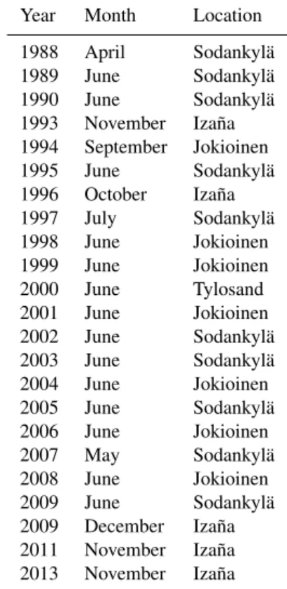
The instruments need to be calibrated regularly to keep track of possible changes in their characteristics and the effect of these changes on the ozone measurements. Calibration can be done at the instrument’s home institute against a well-calibrated reference instrument or the instrument can be moved to take part in a calibration campaign where the instrument can be calibrated against a reference instrument or by using a Langley extrapolation method. The calibration history of the Brewer no. 037 is presented in Table 1. The main characteristics to be redefined are the extraterrestrial constant (ETC), the ratio of measurements from the inter-nal calibration lamp at ozone measurement wavelengths, the wavelength setting for ozone measurements, the instrument function, and the differential absorption coefficient (α).

The ETC tells what the instrument would measure if there was no ozone between the instrument and the Sun. It is de-pendent on the spectral response of the instrument and the change in ETC is monitored by measuring the intensities at the same wavelengths from an internal calibration lamp. In the calibration campaign, the ETC and lamp reference value (R6sl,ref) are determined. If these values behave the same as in the last calibration, any change in the lamp in-tensity ratios is considered as a change in the instrument re-sponse and not a change in the lamp, and thus the time series between calibrations must be corrected for ETC changes as indicated by the changes in the lamp value.

The optimal grating position for ozone measurements is searched by measuring ozone with several positions close to the expected one. The wavelength scale for the micrometer positions is determined by measuring a set of known emis-sion lines from different discharge lamps, for example mer-cury and cadmium lamps. From these lamp measurements the instrument function is also retrieved. The differential ab-sorption coefficient is calculated for the exact operational

Table 1.Brewer no. 037 calibration history (partly adopted from IOS, 2015).

Year Month Location

1988 April Sodankylä 1989 June Sodankylä 1990 June Sodankylä 1993 November Izaña 1994 September Jokioinen 1995 June Sodankylä 1996 October Izaña 1997 July Sodankylä 1998 June Jokioinen 1999 June Jokioinen 2000 June Tylosand 2001 June Jokioinen 2002 June Sodankylä 2003 June Sodankylä 2004 June Jokioinen 2005 June Sodankylä 2006 June Jokioinen 2007 May Sodankylä 2008 June Jokioinen 2009 June Sodankylä 2009 December Izaña 2011 November Izaña 2013 November Izaña

wavelengths as a convolution between the instrument func-tion and the ozone absorpfunc-tion cross secfunc-tion.

In addition to these annual or biennial checks, the dead time of the photomultiplier is constantly monitored. The tem-perature dependence has been characterized already at the factory by the manufacturer. The neutral density filter wave-length dependence has also been measured more frequently lately but no corrections have been applied this far.

Quality control

Quality control includes procedures to ensure the instrument is measuring in the ideal manner, the measurements are not stopped or obstructed, and all the changes in the instrument are recorded.

To ensure the view is not obstructed and the sunlight is transmitted ideally inside the instrument, the window is regu-larly manually cleaned using isopropyl alcohol. For the snow and rain, a blower has been installed that keeps the window clear except for the heaviest snowfalls. After heavy snow-fall, a manual cleaning is required and the situation can be checked from a webcam installed to see the Brewer at all times.

(4)

wavelength selection for accurate measurements and for en-suring the correct behavior of the stepper motors moving the grating. In Sodankylä, the measurements are usually made before each spectral scan where the stepper motors make numerous small steps to scan a big wavelength range with 0.5 nm interval. This ensures the measurements are always made at the exact wavelengths that are expected.

The standard lamp is measured daily for the same wave-lengths that are used in ozone measurements. This assures all the changes in the instrument response are recorded. As-suming the lamp does not change, the value measured from the lamp corresponds to a change in the solar measurements. In a calibration campaign, the lamp measurements are re-viewed to check if the lamp measurement changes are due to a change in the lamp or due to a change in the instrument. Ozone measurements are corrected respectively.

Because the Brewer is also used for spectral UV measure-ments, the changes in the response are followed very care-fully by measuring a 1000 W calibration lamp in a dark room every 6 weeks. After each calibration, before the instrument returns to the measurement site, the tracker is opened and the friction wheel rotating the tracker is cleaned to allow the maximum friction and to ensure there is no slipping and los-ing steps which would result in poor azimuthal pointlos-ing ac-curacy.

To ensure the maximum intensity and thus the maximum contrast in the measurements, the orientation of the tracker and the zenith prism need to be checked regularly. This pro-cedure is called sighting. The instrument is oriented towards the Sun and the entrance slit is viewed from a view port on top of the instrument. If the instrument orientation is perfect, the picture of the Sun is centered around the entrance slit. If this is not the case, the azimuth tracker and zenith prism motors are commanded from buttons on the side of the in-strument casing to turn the inin-strument to achieve perfect ori-entation.

For an accurate orientation check, a human eye is needed, but for a rough check, an automatic routine measurement has been developed. In this routine the intensity of the light through the entrance slit is measured in the original position and in positions a few motor steps away from the original one. The maximum intensity is regarded as the optimum ori-entation and changes are suggested if necessary by the oper-ating software.

Since the beginning of 2015, a database system called IDEAS has been in use to enhance the continuity and quality of the data. The system parses the raw data files and updates in approximately 10 min intervals. Warnings are raised and sent by e-mail if there are signs in the data for misbehavior of the instrument, for example if the wavelength calibration is too much off of the reference value. This warning system ensures the erroneous behavior of the instrument is noticed as soon as possible and corrective action can be taken.

3 Data handling

3.1 Data flow and data storage

Data are collected by the operating computer controlling the Brewer. At this point the data consist of raw counts and pre-liminary data reduction including not only the measurements of ozone but also the wavelength calibration and stability check information. These data are retrieved to a local server once every 5 min. Another server hosting a database system IDEAS, collects the data from the primary local server every 5 min.

The processing of the final products that are sent to the World Ozone and Ultraviolet Radiation Data Cen-tre (WOUDC) and to the FMI-ARC database http://litdb.fmi. fi still require human interaction. The data are collected from the primary local server to a personal computer and pro-cessed with software described in Sect. 3.2. There are rules to assure the quality of the data (Sect. 3.3) but some erro-neous measurements must still be filtered out by the human eye. At the moment, the data are available in the WOUDC database until May 2010 and the update for Sodankylä data will be made when the quality assurance is finished.

Finland is participating in Eubrewnet COST action (COST-ES1207, http://www.eubrewnet.org) and the Brewer data are sent from the primary local server to the Eubrewnet database every 20 min. The database is under development and not fully operational at this moment. When operational, the database will receive Brewer raw data from all the par-ticipating countries and the final products will be processed by a central computer. This way the data will be consistent through the whole network.

3.2 Algorithm

For all ozone measurement procedures, the raw data in-clude total counts from the photomultiplier for seven po-sitions of the slit mask, F0–F6. To retrieve vertical ozone columns, O3Brewer software written in Delphi language by Martin Stanek is used (Stanek, 2015). The retrieval process is described below.

Before the physical modeling of the absorption itself, the raw counts are first turned into photon count ratesC(photons per second) (SCI-TEC Instruments Inc., 1999). First, the dark counts are removed and the integration time for each slit ex-posure is taken into account in term 2/IT, and CY is the num-ber of slit exposure cycles. Dark countsF1are measured at slit mask position 1, where the exit slit is closed. The photon count rateCi for slit mask positionibecomes

Ci=

2×(Fi−F1)

(5)

The photomultiplier has a dead time (DT), a time it takes it to recover from a hit by a photon to be able to count another photon. The effect is assumed to follow the Poisson statistics and hence the equation

Ci,m=Ci,t×e−Ci,t×DT, (2)

whereCi,mis the measured photon count rate andCi,tis the true photon count rate. The first estimate for the true photon count rate is given by

Ci,t,1=Ci,m×eCi,m×DT. (3)

After this, a better estimate is calculated by plugging the first estimate in the original equation

Ci,t,2=Ci,m×eCi,t,1×DT. (4)

This is repeated eight times and the result is expected to con-verge until then, makingCi,t,9the final estimate forCi,t.

Later will be shown that, when calculating ozone, we are dealing with logarithms of irradiance ratios. For this reason the photon count rates are converted to logarithmic scale,Ci,l

Ci,l=104×log10 Ci,t

. (5)

The response of the instrument may change according to the change in temperature inside the instrument. The effect is as-sumed linear and has been characterized at the factory. Cor-rected photon count rateCi,tcwill be

Ci,tc=Ci,l+(TCi)×T , (6)

whereT is temperature and TCiis the wavelength-dependent

temperature correction coefficient.

The final instrumental correction will be neutral density correction. This actually does not affect the ozone calculation as the attenuation is assumed to be wavelength independent. The effect of filter non-neutrality has been found very small in recent calibrations. The final photon count rateCi,fwill be

Ci,f=Ci,tc+NF, (7)

whereNFis the 10 000 times the 10-based logarithm of at-tenuation ratio of the filter.

The physical model of retrieval from final photon count rates to total ozone column, well described by Savastiouk (2006), is based on the Beer–Lambert law considering Rayleigh scattering and scattering by aerosols, as well as ab-sorption by sulfur dioxide and ozone. The data from slit mask position 0 are not taken into account so using the other five (positions 2–6) wavelengths, a set of wavelength-dependent weighting coefficients are found such that the ozone calculus is, in theory, not affected by sulfur dioxide or aerosols. For ozone, the coefficients are such that only four wavelengths (positions 3–5) are needed. The final photon count rates are corrected for Rayleigh scattering according to equation

Ci=Ci,f+

BEi×µr×P

1013 , (8)

whereBEiis Rayleigh correction coefficient for slit mask

po-sitioni. TheBEiused are the original ones calculated by the

instrument designer based on Bates (1984).P is the pressure of the instrument location, set to 1000 mbar for Sodankylä.

µr is the air mass factor for Rayleigh scattering, calculated

from

µr=sec{arcsin[(6370/6375)×sin(A)]}, (9)

whereAis the solar zenith angle at the time of the measure-ment. The double ratioR6 affected only by ozone is calcu-lated from Rayleigh corrected photon count ratesCias

R6= −C3+0.5×C4+2.2×C5−1.7×C6. (10) Total ozone columnXO3, is retrieved from the ratio as

XO3 =(R6−ETC+SL)/ µO3×α

, (11)

where extraterrestrial constant ETC and differential absorp-tion coefficientαare constants determined in calibration.SL

is the change inR6 value measured from a calibration lamp. For this, a reference valueR6sl,refis determined during cali-bration campaign and the changes are followed by measuring this ratioR6sl several times per day. The lamp is assumed not to change and so the changes should reflect changes in the ETC. The assumption is then checked at the next calibra-tion when also the new reference value is determined. The correction factor SL is based on daily mean valueR6slas

SL=R6sl,ref−R6sl. (12)

Ozone air mass factorµO3, describes the path length that the

light has to travel compared to a thickness of the ozone layer right above us. For the calculation, ozone is considered to lie in a thin layer at the altitude of 22 km. This makes the air mass factor

µO3=sec{arcsin[(6370/6392)×sin(A)]}, (13)

whereAis the solar zenith angle.

For the focused sun measurements fz, the algorithm is identical to that of the direct sun. Before calculating the R6 however, the photon count rate measured 0.5◦off of the Sun is deducted from the photon count rate measured from the di-rect sun. This is made to counter the effect of multiply scat-tered light reaching the instrument from the same direction than the direct light (Josefsson, 1992).

(6)

1988 1990 1992 1994 1996 1998 2000 2002 2004 2006 2008 2010 2012 2014 150

200 250 300 350 400 450 500 550

Year

TOC (DU)

Daily total ozone value Spring minimum value Spring maximum value

Figure 1.Total ozone column daily average time series with spring time extreme values highlighted for each year. For the spring, minima and maxima measurements from March and April are considered.

ozone retrieval. As the weighting coefficients in the algo-rithm have been chosen to disregard any absorption effects that are linear with wavelength, there should not be a remark-able difference between focused moon and direct sun mea-surements. After comparing solar and lunar measurements, Kerr (1989) concluded that the ETC and the differential ab-sorption coefficient α are the same for both measurement types.

The processing of the zenith sky measurements is based on the comparison of zenith sky (zs) and direct sun mea-surements (ds) (Muthama et al., 1995). A polynomial will be fitted between a number of near-simultaneous zs and ds measurements so that using theXO3 from ds measurements

a best-possible set of coefficientsatoiare found for relation

R6zs−ETC=a+b×µ+c×µ2+d×X+e×Xµ +f×Xµ2+g×X2+h×X2µ+i×X2µ2. (14)

These coefficients depend on the instrument and on the mea-surement location. For Brewer no. 037 the fitting of the co-efficients, the so-called sky chart, has been done by Karhu (1995).

The daily value is calculated as an average of measure-ments that meet the filtering criteria (see Sect. 3.3). Only one type of measurement is used for one daily value. The measurement types are ranked by their expected quality so that the order is ds, fz, zs, fm. The measurements of lower rank are only used if there are no measurements at the higher level. The ranking is justified by the assumptions that focused sun and moon measurements are more prone to errors due to small deviations in pointing accuracy and zs is more prone to errors due to retrieval algorithm based on a non-physical model.

3.3 Quality assurance

To assure the quality of the data, some automatic data filter-ing rules have been obeyed. The measurement routine for one ozone value has five consecutive measurements. The stan-dard deviation among these five measurements is not allowed to be more than 3 DU (Dobson units) in ds, zs, or fz measure-ments. For moon measurements the deviation is allowed to be 5 DU. The air mass factor has been limited to 3.8 for ds and to 3.0 for zs measurements to avoid the effects of stray light but to allow measurements to start as early as possible in the spring. For focused sun measurements, the air mass limit is set to 6 and for moon measurements to 3.5. Before submitting the data to the database, it is also inspected vi-sually for obvious spikes or other suspicious behavior. The random errors of individual observations are within±1 % in about 90 % of all measurements (Fioletov et al., 2005).

4 Demonstration of the data set

(7)

1990 1995 2000 2005 2010 0

10 20 30

Year

Daily TOC value availability

200 250 300 350 400 450 500 550

Monthly mean TOC (DU)

ds zs fz fm

Figure 2.Upper panel shows the monthly mean ozone calculated from daily values. The amount of daily values available for each month is shown in the lower panel. Different measurement styles have been color coded to show which type of measurements have been used for monthly mean value.

1990 1992 1994 1996 1998 2000 2002 2004 2006 2008 2010 2012 2014

−80 −60 −40 −20 0 20 40 60

Year

Monthly mean − Mean of monthly means (DU), March

Figure 3.The difference of March monthly mean each year to the all-time March mean.

higher. As a result, the ozone reaches its minimum during late autumn before a new buildup begins. However, the spring minimum is still the best indicator for the extent of chemi-cal destruction of the ozone layer. The high values of Febru-ary 1989 stand out from the time series but the data from the same date from TOMS instrument aboard the Nimbus-7 satellite confirm the total amount of ozone was very high.

Monthly mean values have been presented in Fig. 2. In the figure, the number of daily values available for a partic-ular monthly value is also presented. Overall, from all daily values, 77 % are based on ds measurements and 14 % on zs measurements. Winter months are sporadically covered by focused moon measurements. While no significant trend is observed in the monthly mean values, the March monthly mean plot (Fig. 3) suggests that in the beginning of the 1990s there was a period of strong spring ozone depletion and af-ter 1997 there has been huge variability between cold and

Figure 4.Ten days’ running average of daily values 1988–2014 for each day of the year.

warm winters. The monthly mean of March is affected by the intensity of the chemical depletion and the persistence of the polar vortex and thus gives a bit more insight on the extent of the depletion than just the minimum total ozone column measured.

(8)

account-Jan Feb Mar Apr May Jun Jul Aug Sep Oct Nov Dec Jan 0

20 40 60 80 100 120

Date

Amount of daily measurements

Mean, ds Max, ds Mean, zs Max, zs Mean, fz Max, fz Mean, fm Max, fm

Figure 5.The seasonal variability of the amount of measurements. Solid lines represent the mean amount of measurements of each type for each day of the year. The maximum amount for any year for this certain day of year has been plotted in dashed lines in the color representing the measurement type.

ing for the dynamical and chemical variability. They found that total ozone amounts in the stratosphere correlate highly with proxies for the stratospheric circulation, polar ozone de-pletion, and tropopause height.

The daily ozone climatology is depicted in Fig. 4. The main features are the accumulation of ozone during the win-ter and early spring and the decline during the summer ow-ing to the atmospheric circulation patterns and their seasonal changes (Weatherhead et al., 2005). The variability is very large in spring as the location, timing, and persistence of the polar vortex hugely affect the transportation and chem-ical loss of ozone. The uncertainties are larger for the deep winter months as the only measurement mode available is the focused moon procedure.

Figure 5 shows mean and maximum daily amounts of dif-ferent types of measurements and gives another view on mea-surement availability. From the dashed lines depicting max-imum amounts it can be seen that direct sun measurements are more frequent than zenith sky measurements when the sky is clear. However, because of clouds the mean amounts of zenith sky measurements are a bit higher during the summer. The peak in the maximum amounts at midsummer is from the calibration campaign in 2003. During the calibration, direct sun measurements are prioritized and UV scans are omitted. This permits over 100 direct sun measurements to be made during 1 day. Normally, a clear day with regular UV scans can have up to 75 direct sun measurements. Even though the clouds seem to obstruct on average one third of the possible ds measurements, a high portion of the daily values is based on them as there usually is a possibility during the day to get some successful direct sun measurements. The availabil-ity of ds and zs measurements in the spring and in the fall are

affected by the air mass factor limits of 3.8 and 3.0, respec-tively. The focused sun and moon measurements are, on av-erage, very rare but some days can give up to 20 good-quality measurements during the time when direct sun or zenith sky measurements are impossible or too unreliable.

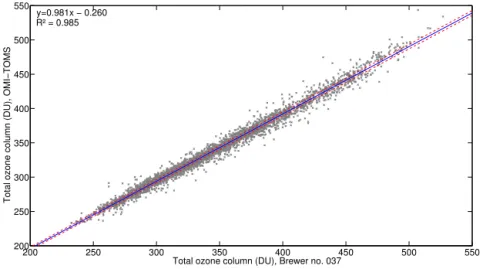
In Fig. 6 is the comparison of Brewer no. 037 and the Ozone Monitoring Instrument (OMI) on board the NASA EOS-AURA satellite between the years 2004 and 2014, showing a systematic difference of about 1.9 %. Sodankylä Brewer data have been used in several satellite comparisons (e.g., Kyrö, 1993; Balis et al., 2007; Damiani et al., 2012) and in comparison to other ground-based instruments (e.g., Vigouroux et al., 2008). Sodankylä also hosted two total ozone column intercomparison campaigns in the springs of 2006 and 2007, aiming to characterize and tackle the mea-surement challenges caused by low solar elevation angles (McPeters et al., 2006). A follow-up CEOS Intercal Nordic campaign was arranged consisting of measurement periods at Sodankylä, for low solar elevation measurements, and at Izaña for high solar elevation measurements and laboratory characterization (Karppinen et al., 2015).

5 Conclusions

(9)

200 250 300 350 400 450 500 550 200

250 300 350 400 450 500 550

Total ozone column (DU), OMI−TOMS

Total ozone column (DU), Brewer no. 037 y=0.981x − 0.260

R² = 0.985

Figure 6.Comparison of Brewer no. 037 direct sun measurements and OMI satellite data using TOMS retrieval algorithm. The Brewer

reference value was the closest direct sun measurement with a maximum limit of 1 h difference in the measurement times.

data will be available in WOUDC database as well as in http://www.litdb.fmi.fi. Data are also sent to the Eubrewnet database where the Brewer community will set up best possi-ble data processing algorithm to achieve coherent total ozone data across the Eubrewnet network. Sodankylä data are valu-able for Arctic ozone studies and for validating other ozone measurements at high latitudes.

Acknowledgements. Authors thank Johanna Tamminen for the valuable comments during the writing process. Authors also thank Martin Stanek for the review and comments on the ozone retrieval algorithm as well as for clarification on several data handling issues of Brewer data. Authors are grateful to Volodya Savastiouk for setting up the IDEAS database software and for the help on clarifying any questions we have had about Brewer software or hardware issues.

Edited by: N. Partamies

References

Balis, D., Kroon, M., Koukouli, M. E., Brinksma, E. J., Labow, G., Veefkind, J. P., and McPeters, R. D.: Validation of Ozone Monitoring Instrument total ozone column measure-ments using Brewer and Dobson spectrophotometer ground-based observations, J. Geophys. Res.-Atmos., 112, d24S46, doi:10.1029/2007JD008796, 2007.

Bates, D.: Rayleigh scattering by air, Planet. Space Sci., 32, 785– 790, doi:10.1016/0032-0633(84)90102-8, 1984.

Bhartia, P. K., Heath, D. F., and Fleig, A. F.: Observation of anoma-lously small ozone densities in south polar stratosphere dur-ing October 1983 and 1984, Paper presented at the Symposium on Dynamics and Remote Sensing of the Middle Atmosphere, 5th Scientific Assembly, 5–17 August 1985, Prague, Czechoslo-vakia, 1985.

Brewer, A. W. and Kerr, J. B.: Total ozone measurements in cloudy weather, Pure Appl. Geophys., 106, 928–937, doi:10.1007/BF00881043, 1973.

Damiani, A., Simone, S. D., Rafanelli, C., Cordero, R., and Lau-renza, M.: Three years of ground-based total ozone measure-ments in the Arctic: Comparison with OMI, GOME and SCIA-MACHY satellite data, Remote Sens. Environ., 127,162 –180, doi:10.1016/j.rse.2012.08.023, 2012.

Farman, J. C., Gardiner, B. G., and Shanklin, J. D.: Large losses of total ozone in Antarctica reveal seasonal ClOx/NOxinteraction,

Nature, 315, 207–210, 1985.

Fioletov, V. E., Kerr, J. B., McElroy, C. T., Wardle, D. I., Savastiouk, V., and Grajnar, T. S.: The Brewer reference triad, Geophys. Res. Lett., 32, l20805, doi:10.1029/2005GL024244, 2005.

IOS: Internationa Ozone Services website/Brewer037, http://www. io3.ca/Calibrations/Brewer/037, last access: 24 November 2015. Josefsson, W. A. P.: Focused sun observations using a Brewer ozone spectrophotometer, J. Geophys. Res.-Atmos., 97, 15813–15817, doi:10.1029/92JD01030, 1992.

Karhu, J. M.: Ilmakehän otsonin mittaamisesta: Zeniitti-nomogrammit Brewer-spektrometrille n:o 37 vuosien 1990– 1994 ds- ja zs-otsonimittausten perusteella, Master’s thesis, Physics department, University of Oulu, Oulu, Finland, 63 pp., 1995.

Karppinen, T., Redondas, A., García, R., Lakkala, K., McEl-roy, C., and Kyrö, E.: Compensating for the Effects of Stray Light in Single-Monochromator Brewer Spec-trophotometer Ozone Retrieval, Atmos.-Ocean, 53, 66–73, doi:10.1080/07055900.2013.871499, 2015.

Kazadzis, S., Bais, A., Kouremeti, N., Gerasopoulos, E., Garane, K., Blumthaler, M., Schallhart, B., and Cede, A.: Direct spec-tral measurements with a Brewer spectroradiometer: absolute calibration and aerosol optical depth retrieval, Appl. Optics, 44, 1681–1690, 2005.

(10)

Int. Ozone Symp., 4–13 August 1988, Göttingen, FRG, 728– 731,1989.

Kipp & Zonen: Brewer Spectrophotometer, Brewer Map, http: //www.kippzonen-brewer.com/community/brewer-map/, last ac-cess: 3 December 2015.

Kivi, R., Kyrö, E., Turunen, T., Ulich, T., and Turunen, E.: Atmo-spheric Trends Above Finland: II Troposhere and Stratosphere, Geophysica, 35, 71–85, 1999.

Kivi, R., Kyrö, E., Turunen, T., Harris, N. R. P., von der Gathen, P., Rex, M., Andersen, S. B., and Wohltmann, I.: Ozonesonde ob-servations in the Arctic during 1989–2003: Ozone variability and trends in the lower stratosphere and free troposphere, J. Geophys. Res.-Atmos., 112, d08306, doi:10.1029/2006JD007271, 2007. Kyrö, E.: Intercomparison of total ozone data from

Nim-bus 7 TOMS, the Brewer UV Spectrophotometer and SAOZ UV-Visible Spectrophotometer at High Latitudes Ob-servatory, Sodankylä, Geophys. Res. Lett., 20, 571–574, doi:10.1029/93GL00806, 1993.

Lebedinsky, A. I., Krasnopolsky, V. A., and Kryska, A.: Moon and Planets, North Holland Publ. Co., Proc. 7th COSPAR Confer-ence, May 1964, FlorConfer-ence, Italy, 59–64, 1967.

Lucas, R., McMichael, T., Smith, W., and Armstrong, B.: So-lar Ultraviolet Radiation: Global burden of disease from so-lar ultraviolet radiation, Environmental burden of disease series no. 13, WHO Document Production Service, Geneva, Switzer-land, 2006.

Lucke, R. L., Henry, R. C., and Fastie, W. G.: Far-ultraviolet albedo of the moon, Astron. J., 81, 1162–1169, doi:10.1086/112000, 1976.

Manney, G. L., Santee, M. L., Rex, M., Livesey, N. J., Pitts, M. C., Veefkind, P., Nash, E. R., Wohltmann, I., Lehmann, R., Froide-vaux, L., Poole, L. R., Schoeberl, M. R., Haffner, D. P., Davies, J., Dorokhov, V., Gernandt, H., Johnson, B., Kivi, R., Kyro, E., Larsen, N., Levelt, P. F., Makshtas, A., McElroy, C. T., Naka-jima, H., Parrondo, M. C., Tarasick, D. W., von der Gathen, P., Walker, K. A., and Zinoviev, N. S.: Unprecedented Arctic ozone loss in 2011, Nature, 478, 469–475, doi:10.1038/nature10556, 2011.

McPeters, R. D., Bojkov, B., Bhartia, P. K., Kyro, E., and Zehner, C.: The Sodankylä Total Ozone Intercomparison and Validation Campaign (SAUNA), AGU Spring Meeting Abstracts, Abstract A41A-04, 23–26 May 2006.

Molina, M. J. and Rowland, F. S.: Stratospheric sink for chloroflu-oromethanes: chlorine atom-catalysed destruction of ozone, Na-ture, 249, 810–812, doi:10.1038/249810a0, 1974.

Müller, R.: Stratospheric Ozone Depletion and Climate Change, in: chap. 1, Introduction, The Royal Society of Chemistry, Thomas Graham House, Cambridge, UK, 3–9, 2012.

Muthama, N. J., Scimia, U., Siani, A. M., and Palmieri, S.: Toward optimizing Brewer zenith sky total ozone measurements at the Italian stations of Rome and Ispra, J. Geophys. Res.-Atmos., 100, 3017–3022, doi:10.1029/94JD02389, 1995.

Rex, M., Harris, N. R. P., von der Gathen, P., Lehmann, R., Braa-then, G. O., Reimer, E., Beck, A., Chipperfield, M. P., Alfier, R., Allaart, M., O’Connor, F., Dier, H., Dorokhov, V., Fast, H., Gil, M., Kyro, E., Litynska, Z., Mikkelsen, I. S., Molyneux, M. G., Nakane, H., Notholt, J., Rummukainen, M., Viatte, P., and Wenger, J.: Prolonged stratospheric ozone loss in the 1995–

96 Arctic winter, Nature, 389, 835–838, doi:10.1038/39849, 1997.

Rex, M., Salawitch, R. J., Harris, N. R. P., von der Gathen, P., Braathen, G. O., Schulz, A., Deckelmann, H., Chipperfield, M., Sinnhuber, B.-M., Reimer, E., Alfier, R., Bevilacqua, R., Hop-pel, K., Fromm, M., Lumpe, J., Küllmann, H., Kleinböhl, A., Bremer, H., von König, M., Künzi, K., Toohey, D., Vömel, H., Richard, E., Aikin, K., Jost, H., Greenblatt, J. B., Loewenstein, M., Podolske, J. R., Webster, C. R., Flesch, G. J., Scott, D. C., Herman, R. L., Elkins, J. W., Ray, E. A., Moore, F. L., Hurst, D. F., Romashkin, P., Toon, G. C., Sen, B., Margitan, J. J., Wennberg, P., Neuber, R., Allart, M., Bojkov, B. R., Claude, H., Davies, J., Davies, W., De Backer, H., Dier, H., Dorokhov, V., Fast, H., Kondo, Y., Kyrö, E., Litynska, Z., Mikkelsen, I. S., Molyneux, M. J., Moran, E., Nagai, T., Nakane, H., Parrondo, C., Ravegnani, F., Skrivankova, P., Viatte, P., and Yushkov, V.: Chemical depletion of Arctic ozone in winter 1999/2000, J. Geophys. Res.-Atmos., 107, 8276, doi:10.1029/2001JD000533, 2002.

Savastiouk, V.: Improvements to the direct-sun ozone observations taken with the Brewer spectrophotometer, PhD thesis, York Uni-versity, Toronto, Ontario, Canada, 44–57, 2006.

SCI-TEC Instruments Inc.: Brewer MKII Spectrophotometer, oper-ator’s manual, Saskatoon, Sask., Canada, 109–112, 1999. Stanek, M.: O3Brewer, http://www.o3soft.eu/o3brewer.html, last

access: 24 November 2015.

Teramura, A. and Ziska, L.: Ultraviolet-B Radiation and Photosyn-thesis, in: Photosynthesis and the Environment, vol. 5 of Ad-vances in Photosynthesis and Respiration, edited by: Baker, N., Springer Netherlands, 435–450, doi:10.1007/0-306-48135-9_18, 1996.

Vigouroux, C., De Mazière, M., Demoulin, P., Servais, C., Hase, F., Blumenstock, T., Kramer, I., Schneider, M., Mellqvist, J., Strand-berg, A., Velazco, V., Notholt, J., Sussmann, R., Stremme, W., Rockmann, A., Gardiner, T., Coleman, M., and Woods, P.: Eval-uation of tropospheric and stratospheric ozone trends over West-ern Europe from ground-based FTIR network observations, At-mos. Chem. Phys., 8, 6865–6886, doi:10.5194/acp-8-6865-2008, 2008.

Weatherhead, B., Tanskanen, A., Stevermer, A., Andersen, S. B., Arola, A., Austin, J., Bernhard, G., Browman, H., Fioletov, V., Grewe, V., Herman, J., Josefsson, W., Kylling, A., Kyró, E., Lindfors, A., Shindell, D., Taalas, P., Tarasick, D., Dorokhov, V., Johnsen, B., Kaurola, J., Kivi, R., Krotkov, N., Lakkala, K., Lenoble, J., and Sliney, D.: Ozone and Ultraviolet Radiation, in: Arctic Climate Impact Assessment, chap. 5, edited by: Symon, C., Arris, L., and Hea, B., Cambridge University Press, Cam-bridge, p. 154, 2005.

WMO: Scientific Assessment of Ozone Depletion: 1985, Global Ozone Research and Monitoring Project-Report No. 16, Geneva, Switzerland, 1985.

(11)