Extrapolating future Arctic ozone losses

(1)

ACPD

4, 3227–3248, 2004

Extrapolating future Arctic ozone losses

B. M. Knudsen et al.

Title Page

Abstract Introduction

Conclusions References

Tables Figures

◭ ◮

Back Close

Full Screen / Esc

Print Version

Interactive Discussion

©EGU 2004

Atmos. Chem. Phys. Discuss., 4, 3227–3248, 2004 www.atmos-chem-phys.org/acpd/4/3227/

SRef-ID: 1680-7375/acpd/2004-4-3227 © European Geosciences Union 2004

Atmospheric Chemistry and Physics Discussions

Extrapolating future Arctic ozone losses

B. M. Knudsen1, S. B. Andersen1, B. Christiansen1, N. Larsen1, M. Rex2, N. R. P. Harris3, and B. Naujokat4

1

Danish Meteorological Institute, Denmark 2

Alfred Wegener Institute for Polar and Marine Research, Germany 3

European Ozone Research Coordinating Unit, United Kingdom 4

Free University of Berlin, Germany

(2)

ACPD

4, 3227–3248, 2004

Title Page

Tables Figures

◭ ◮

Back Close

Full Screen / Esc

Print Version

©EGU 2004

Abstract

Future increases in the concentration of greenhouse gases and water vapour are likely to cool the stratosphere further and to increase the amount of polar stratospheric clouds (PSCs). Future Arctic PSC areas have been extrapolated using the highly sig-nificant trends in the temperature record from 1958–2001. Using a tight correlation

5

between PSC area and the total vortex ozone depletion and taking the decreasing amounts of ozone depleting substances into account we make empirical estimates of future ozone. The result is that Arctic ozone losses increase until 2010–2020 and only decrease slightly up to 2030. This approach is an alternative method of prediction to that based on the complex coupled chemistry-climate models (CCMs).

10

1. Introduction

The success of the Montreal Protocol and its amendments should lead to decreas-ing amounts of ozone depletdecreas-ing substances in the future. This in turn would lead to decreased ozone depletion if other factors remained unchanged. However, the stratosphere has been cooling for decades and some measurements suggest that the

15

amount of water vapour in the stratosphere is increasing. Both these factors would tend to increase the ozone depletion in the Arctic vortex. Predicting the future ozone layer therefore involves a delicate balance between competing processes.

The tools used to predict future ozone depletion are chemistry-climate models (CCMs). These CCMs, while physically based, parameterise many important

pro-20

cesses affecting the ozone layer, and do not include others. There is no agreement between models as to whether ozone will increase or decrease in the future. One of the reasons is that the current CCMs have di_fficulty in calculating correct polar temper-atures, which are essential for determining the amount of ozone depletion. The range of model predictions of Arctic temperatures is currently too wide to make reliable

pre-25

(3)

ACPD

4, 3227–3248, 2004

Title Page

Tables Figures

◭ ◮

Back Close

Full Screen / Esc

Print Version

©EGU 2004

Arctic (WMO, 2003).

CCMs also have di_fficulties in representing two other important processes for po-lar ozone loss: the increase in stratospheric water vapour and the formation mecha-nism for solid type polar stratospheric clouds (PSCs). The observed increase in water vapour (Oltmans et al., 2000; Rosenlof et al., 2001) may have contributed substantially

5

(Forster and Shine, 2002) to the observed cooling in the stratosphere (Ramaswamy et al., 2001; WMO, 2003). Yet, current CCMs include little more than that∼1/3 of the

trend in water vapour, which is due to increasing methane (WMO, 2003). In fact cur-rent chemistry-climate models do not reproduce either today’s amounts of Arctic PSCs or the large increase since the 1960s (Austin et al., 2003; WMO, 2003; Pawson and

10

Naujokat, 1997, and updates). Even if analysed temperatures are used in state-of-the-art chemical transport models the observed ozone depletion is not modelled correctly (Guirlet et al., 2000; Rex et al., 2004). This may be due to the fact that the formation of solid type PSC’s is not well understood (Tolbert and Toon, 2001), making it di_fficult e.g. to model denitrification due to sedimentation of PSC particles, which can increase

15

ozone depletion substantially (Waibel et al., 1999).

We thus have limited confidence in the predictions of future Arctic ozone losses made with even the best present day CCMs. Therefore, we have developed an alternative approach based on the observed behaviour of the stratosphere over the past 40–50 years. We base this approach on the tight correlation between PSCs and the total

20

vortex ozone depletion observed by Rex et al. (2004). We do the extrapolation into the future using the highly significant increase in PSC occurrence (due to cooling in the Arctic vortex) from 1958–2001, taking into account the decreasing amounts of ozone depleting substances in the future. In this simplistic approach the water vapour trend and denitrification is included implicitly. Although such simple extrapolations have large

25

(4)

ACPD

4, 3227–3248, 2004

Title Page

Tables Figures

◭ ◮

Back Close

Full Screen / Esc

Print Version

©EGU 2004

2. Data

2.1. Temperatures and calculation of PSC area

The Free University of Berlin (FUB) has made historical wintertime analyses of the NH stratosphere, which primarily use radiosonde data, from July 1965 to June 2001 (Labitzke et al, 2002; Pawson and Naujokat, 1997). They are available in a 10◦

latitude-5

longitude grid. Since 1977 a 5◦ grid was used, but for consistency the data set was thinned to the 10◦ _grid.

The ECMWF 40 year reanalyses (ERA40) (Simmons and Gibson, 2000) covers the period 1957–2002. It uses a 3D variational analysis at T159 resolution and 60 levels in the vertical. The data were extracted in a 5◦ _{lat-lon grid from T21 truncated fields.}

10

These data were then thinned to the 10◦FUB grid.

There are no long term observational records of PSCs suitable for this analysis. Accordingly the PSC area is defined here as the area where the temperature is below the nitric acid trihydrate condensation temperatures (T_NAT)(Hanson and Mauersberger, 1988). The quality of the predicted temperatures below T_NAT has been assessed by

15

comparison of both the analyses and the first guess fields (i.e. the 6-h forecasts from the last analysis, which is independent from individual radiosondes) to radiosondes. The extent of such low temperatures at 50 hPa was 6–10 and 1–2% lower than the radiosonde extent in 1995/1996 and 1996/1997 (Knudsen, 2003), respectively. The NH winter averaged PSC extent using FU-Berlin data is 11 and 5% higher than the

ERA-20

40 PSC extent in 1995/1996 and 1996/1997, respectively. Thus, the both the ERA40 and the FU-Berlin PSC extent agrees well with observations. The ERA-15 reanalysis (Gibson et al., 1997), which has also been used, does not have a comparable accuracy of temperatures (Knudsen, 1996).

The FUB data are valid for 0:00 UT, whereas the ECMWF data are calculated for

25

12:00 UT. Tests show that this has only a minor e_ffect on the PSC areas. The same is true for PSC areas calculated at higher resolution.

(5)

anal-ACPD

4, 3227–3248, 2004

Title Page

Tables Figures

◭ ◮

Back Close

Full Screen / Esc

Print Version

©EGU 2004

yses. In 1957, the International Geophysical Year, the number of radiosondes became comparable to the current number. In 1964 the former Soviet Union started supplying radiosonde data above 100 hPa and in 1979 satellite data became available. However, the averaged PSC area over the whole winter is a relative robust quantity, which does not depend on small errors. The FU-Berlin analyses have remained almost unchanged

5

during the period and should thus be well suited for trend studies.

2.2. Water vapour

Following Forster and Shine (2002), we have adopted a homogeneous H₂O trend of 0.05 ppmv/year. The reference point is the UARS 1992–1998 HALOE₊MLS clima-tology for February (http://code916.gsfc.nasa.gov/Public/Analysis/UARS/urap/home.

10

html) at 70◦N equivalent latitude. With this trend the 50 hPa H₂O mixing ratios (T_NAT) are 4.40 ppmv (195.0 K) in 1995, 3.65 ppmv (194.3 K) in 1980, 2.85 ppmv (193.2 K) in 1964 and 2.55 ppmv (192.8 K) in 1958. The nitric acid mixing ratio used is the LIMS January value at 76◦N of 9 ppbv. In the SH the 70 hPa 64◦S value of 6 ppbv was cho-sen in May, before denitrification and dehydration sets in. The SH H₂O mixing ratio in

15

May at 70 hPa and 70◦S is also 4.4 ppmv.

3. PSC trends

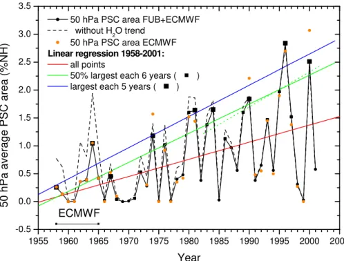
Figure 1 shows the mid December to end of March mean 50 hPa PSC area for FUB and ERA-40 analyses. The FUB and ERA40 data agree quite well in most years. One exception is in 2000, where large temperature biases occurred over the poles in the

20

ERA40 data (Knudsen, 2003). When this figure was prepared the ERA40 reanalyses had not yet been completed. We have therefore used a combined data set with ERA40 data 1958–1965 and FUB data afterwards (solid line).

In the absence of a trend in H₂O, T_NAT would be constant and the PSC areas would follow the dashed black line. The linear regression line though all points, which are

(6)

ACPD

4, 3227–3248, 2004

Title Page

Tables Figures

◭ ◮

Back Close

Full Screen / Esc

Print Version

©EGU 2004

independent, is the solid red line. The PSC areas increase with more than 99.9% confidence (4σ) during the period (von Storch and Zwiers, 1998, Sect. 8.3.7).

The Arctic winter stratosphere is sometimes disrupted by major stratospheric warm-ings, which usually bring an end to the PSC season and limit the ozone loss. The largest ozone losses occur in the cold uninterrupted winters. To examine this group

5

of winters separately, the maximum PSC areas in successive 5-year intervals (2001– 1997, 1996–1992, etc.) are extracted (large squares)(Rex et al., 2004). The first in-terval (1958–1961) is only 4 years long. Linear regression reveals a highly significant (more than 99.99% confidence (8σ)) upward trend in these 9 maximum PSC areas.

Such PSC areas are expected statistically only every fifth winter, so we have also

ex-10

amined the trends of the largest half of the PSC areas in 6-year intervals (squares; 2001–1996, 1995–1990, etc.) which are expected statistically every second winter. These trends are the main focus of this paper.

The first interval (1958–1959) is only 2 years long, and the larger of these two PSC areas is included in the trend calculations. In fact it would also have been chosen in the

15

6-year interval from 1958–1963. Again highly significant upward trends are obtained (8σ). Sensitivity studies reveal that going to 8-year intervals or starting the intervals in

1958 (both for 6 and 8 year intervals) changes the calculated trend by a factor ranging from 0.95–1.04. Going to 4-year intervals changes the calculated trend by a factor of 0.85 and decreases the significance of the trend substantially. This is due to inclusion

20

of the small PSC area in 2001.

Since 1984 the FUB data over data-sparse regions have been supplemented by satellite derived data. We have therefore calculated the trends of the 50% largest PSC areas for the period 1984–2001. The slope is 0.063_±0.032%NH/year (1σ) and

is significant at the 90% confidence limit, when the small numbers of data points are

25

(7)

ACPD

4, 3227–3248, 2004

Title Page

Tables Figures

◭ ◮

Back Close

Full Screen / Esc

Print Version

©EGU 2004

4. Correlation between PSC area and ozone depletion

Vortex averaged ozone depletions in the Arctic from 400–550 K potential temperature have been calculated by Rex et al. (2004), and they form probably the most accurate and consistent data set for Arctic vortex ozone depletions. Although there are certain assumptions involved in this method, it does give a correct depletion in the winter

5

1999/2000 (Lait et al., 2002; Schoeberl et al., 2002). It has been shown that mixing ideally should be taken into account at the bottom of the vortex and below (Knudsen et al., 1998) and in some years even above (Grooß and M ¨uller, 2002).

Rex et al. (2004) found a high correlation between mean PSC volume and mean end-of-winter column ozone depletion. To be able to use the FUB data we here use 50

10

hPa PSC areas instead, and to compare with the Antarctic ozone hole the total vortex depletion in Mt is used instead of the column depletion. Another advantage of using the total vortex depletion in Mt is that this quantity determines how large an influence the vortex depletion has on ozone levels at mid-latitudes after break-up of the vortex (Knudsen and Grooß, 2000; Knudsen and Andersen, 2001). The edge of the vortex

15

used to calculate the vortex area is the position of largest gradient in 475 K PV. The vortex area was averaged in the period mid December to end of March, in which the PSC areas were calculated. In 1997 and 1999 the vortex did not establish at 475 K before around 8 January, so the vortex areas are calculated as of this date.

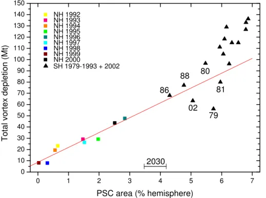
Figure 2 shows the remarkably good correlation (correlation coe_fficient 0.96) of the

20

total depletion with the PSC area for the period 1992–2000 for the NH. Also shown are the 68% confidence limits on the 50% largest PSC areas for 2030. One question is whether this correlation can be extended to these larger PSC areas expected in a future colder stratosphere, as it is possible that we have reached some kind of saturation where larger PSC areas do not lead to larger ozone losses. To investigate this we turn

25

(8)

ACPD

4, 3227–3248, 2004

Title Page

Tables Figures

◭ ◮

Back Close

Full Screen / Esc

Print Version

©EGU 2004

communication). Later years have been omitted because then ERA-15 data would not be available and adding more points in the upper right corner of the plot would not be of any help. The only exception is the year 2002, which was unusually warm with PSC areas close to the NH values.

Possibly the best available estimate of the long-term ozone vortex depletion in the SH

5

is the October mean column ozone from Halley (76◦_{S, 26}◦_{W) (WMO, 1995, updated}

courtesy J. D. Shanklin) minus the 1956–1959 mean (310 DU). The column ozone at Halley is of course lower than in the vortex mean, but so is the climatological mean at Halley.

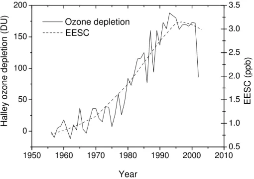
Model calculations (Sinnhuber et al., 2002) show that the ozone loss is proportional

10

to the equivalent e_ffective stratospheric chlorine (EESC) loading, which incorporates bromine. Figure 3 shows that this is a fair assumption for the Antarctic ozone losses. In order to compare to the current NH depletions we have scaled the SH depletions up to the 1992–2000 halogen loading. This is done by dividing the SH depletions by the fraction of EESC in each year relative to the 1992–2000 average. The period during

15

which the average PSC area is calculated is mid July to end of October. This is one month later in the season than in the NH because the SH vortex is much more pole-centred and sunlight reaches Halley later than it reaches the NH vortex. In the SH the PSC areas before mid July would not add to the ozone depletion since dehydration and denitrification would occur anyway. The level used is 70 hPa because the ozone

deple-20

tion in the SH vortex occurs lower than in the NH. The vortex area used is 12.5% of the SH (61◦S equivalent latitude) taken from the 550 K 1979–2000 mean (WMO, 2003). Figure 2 justifies the assumption that further increases in the NH winter averaged PSC areas would lead to further ozone loss.

5. Future ozone losses

25

(9)

ACPD

4, 3227–3248, 2004

Title Page

Tables Figures

◭ ◮

Back Close

Full Screen / Esc

Print Version

©EGU 2004

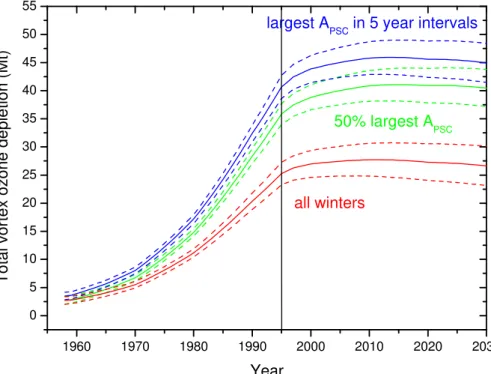
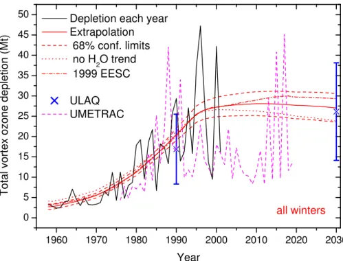
area and ozone depletion from Fig. 2 and scaling the results by the fraction of EESC rel-ative to the 1992–2000 average (WMO, 2003) to allow for decreasing EESC we obtain the future predictions of the ozone losses in Fig. 4. The dashed lines give 68% confi-dence intervals for the means at each year (Von Storch and Zwiers, 1998, Sect. 8.3.10) taking only the uncertainties in the PSC area regressions into account (note that this

5

does not mean that 68% of the depletions will lie within the dashed lines, because indi-vidual depletions have a larger variation than the mean). Almost the same confidence intervals for the future parts of the lines are obtained by using lines crossing the re-gression line at the central year (1979.5) in Fig. 2 with the slope of the rere-gression line

±the standard deviation of the slope. To get 95% confidence limits the line spacing

10

would have to be approximately doubled. Due to the small number of points, the line spacing for the maximum PSC area in 5-year intervals would, however, increase by a factor of 2.14 instead of 2.

The largest PSC areas in 5-year intervals lead to the largest ozone depletion in the future, but such depletion is only expected statistically every 5th year. Generally,

15

we predict that the ozone depletion will increase, reach a maximum between 2010 and 2020, and then decrease slightly before 2030. For comparison, the CCMs do not agree on whether or not ozone depletion will increase in the future and show a substantial recovery by 2030 (Austin et al., 2003; WMO, 2003). It should be noted that by 2030 uncertainties are quite large in any prediction and in particular in our extrapolation.

20

While the ozone depletion in the Arctic vortex might match the amount of ozone depletion in the SH in the warmest years of the 1980s (without the scaling to the 1992– 2000 mean EESC), there is no indication that it will ever reach current levels of total depletion (in Mt) in the Antarctic ozone hole. The Antarctic column depletions (in DU) during the warmest years in the 1980’s were already surpassed in the Arctic in 1996.

25

(10)

ACPD

4, 3227–3248, 2004

Title Page

Tables Figures

◭ ◮

Back Close

Full Screen / Esc

Print Version

©EGU 2004

Soviet Union radiosonde temperatures above 100 hPa are only available since 1964. Further, radiosondes might have had di_fficulties in observing very low temperatures in the early years (Pawson and Naujokat, 1997). However, the FUB period may be biased by 5 out of the first 6 years being warm. It is informative to calculate how often such an event occurs. If the chance of a “warm” winter is 1₂, the chance of at least 5 out of

5

6 winters being warm is 7×(1₂)6=0.11. Such an event is therefore expected every 55

years.

The H₂O trend is not fully explained. Scaife et al. (2003) showed that part of the trend is due to the upward trend in the Southern Oscillation Index (SOI). It is not known, whether the change in the SOI is a temporary natural variation or a more permanent

10

change due to increased greenhouse gases. We have therefore tried to look at the e_ffect on the future predictions if the trend slows down. About 35% of the H₂O trend is due to the trend in methane, which is thought to continue in the future (WMO, 2003). The levelling o_ffof the methane trend in recent years might be due to decreased fossil fuel burning in the former Sovjet Union (Dlugokencky et al., 2003).

15

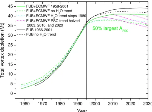
Because of the uncertainties about the H₂O trend (SPARC, 2000) we have studied the sensitivity of the future predictions on the trend. If the H₂O trend is not taken into account in the calculation of the PSC areas, Fig. 5 shows that less ozone depletion would be expected (green dashed line). The prediction based on FUB data only is not as sensitive to the H₂O trend (black dashed line). The best-documented part of the

20

trend goes back to 1980 (Oltmans et al., 2000). The cyan dotted line shows that using this part of the H₂O trend still gives less depletion.

The 1980–2000 trends in H₂O, greenhouse gases, and stratospheric ozone are es-timated to have caused a mid December to mid March 50 hPa high-latitude NH cooling of about 1.1, 0.2, and 0.6 K, respectively (Forster and Shine, 2002; Rosier and Shine,

25

(11)

ACPD

4, 3227–3248, 2004

Title Page

Tables Figures

◭ ◮

Back Close

Full Screen / Esc

Print Version

©EGU 2004

Since our results indicate that the future trend of ozone is close to zero, we would expect the temperature trend to decrease by about 1/3, which would lead to future ozone depletions close to the green dashed line. If the non-methane related part of the H₂O trend were to stop the remaining temperature trend would be about half the 1980–2000 trend. Figure 5 shows that this would lead to a faster recovery of the ozone

5

layer (magenta dash-dotted line). In the last years H₂O has decreased (Rosenlof et al., 2003), but this may be related to changes in the SOI (Scaife et al., 2003). It should be noted that there is no consensus about the attribution of the observed downward trend of the Arctic winter temperatures to the trends in ozone, greenhouse gases, and water vapour (WMO, 2003). If ozone plays a larger role for the decreasing temperatures

10

the future ozone depletions would become smaller, whereas a smaller role for water vapour would increase the confidence in the future predictions.

6. Comparison to models

Rex et al. (2004) show that the SLIMCAT CTM does not reproduce the observed in-crease in ozone depletion with increasing PSC areas and this is likely to apply to CCMs

15

as well. In Fig. 6 we show a prediction of the vortex ozone losses based on the 50 hPa PSC areas from CCM calculations (Austin et al., 2003). These CCM PSC areas equal the average area of temperatures below 195 K and are November–March averages, so our predicted PSC areas have been calculated for this period rather than the mid-December to end March period shown earlier. The red line shows the resulting

pre-20

diction of the ozone depletion, while the red dashed lines give the 68% confidence limits. The black line shows the predicted ozone depletion in individual years based on the actual PSC extent instead of the trend. The CCMs all use an old halogen sce-nario (WMO, 1999), which predicted larger concentrations and therefore more ozone depletion in the future as seen in the figure (red dash-dotted line) for our predictions.

25

(12)

ACPD

4, 3227–3248, 2004

Title Page

Tables Figures

◭ ◮

Back Close

Full Screen / Esc

Print Version

©EGU 2004

ozone depletion. For example, the European Centre Hamburg (ECHAM) models have too large areas with T<195 K due to the common cold-pole problem, but in the ozone

depletion calculations this is resolved by using a nucleation barrier for PSC formation. The ECHAM models predicts a warming of the Arctic vortex in the future due to in-creased planetary wave activity (Schnadt et al., 2002), while the opposite is the case

5

for the University of L’Aquila (ULAQ) and Goddard Institute for Space Studies (GISS) models. This is the main reason for the large differences in the predictions of the future ozone between CCMs.

The results from the ULAQ model (Pitari et al., 2002) are in good agreement with ob-served PSC areas in 1990 and also with the extrapolated results for 2030. The ULAQ

10

model predicts a slight increase in the March-April minimum total ozone in the Arctic from 1990 to 2030 (Pitari et al., 2002, and personal communication) contrary to our prediction in Fig. 6 based on the ULAQ PSC areas only (blue crosses). The results of the Unified Model with Eulerian TRansport And Chemistry (UMETRAC)(Austin and Butchart, 2003) moderately underestimates observed past PSC areas and does not

15

capture the increase since 1975 (dashed magenta line). This may be connected to incorporation of only the methane related part of the H₂O trend and not the (contro-versial) remaining part. For reference our prediction without a H₂O trend in the PSC thresholds is shown in Fig. 6 as the red dotted line. From the UMETRAC PSC area calculations we predict much smaller ozone depletions in the future in agreement with

20

their predictions of the March-April minimum total ozone in the Arctic (Austin et al., 2003).

Of the other 3-D CCMs in WMO (2003) and Austin (2003) the GISS model showed much more ozone depletion than our results by 2010–2020, whereas the remaining models showed substantially less depletion. For the GISS model no PSC areas were

25

available. The GISS model has been criticized for its coarse resolution and simple dynamics, but this may in fact be less important than other model features such as gravity-wave parameterisations (Shindell, 2003).

(13)

ACPD

4, 3227–3248, 2004

Title Page

Tables Figures

◭ ◮

Back Close

Full Screen / Esc

Print Version

©EGU 2004

contrary to our results. Danilin et al. (1998) also predicted little recovery by 2030 in idealized air parcels using a chemical box model forced by a cooling of 1 K/dec. Waibel et al. (1999) found ozone recovery to be substantially delayed due to extensive denitrification caused by a cooling of 5 K. Tabazadeh et al. (2000) argue that severe denitrification in the Arctic is possible in the future with a cooling of 4 K and could

5

enhance ozone loss by up to 30%.

7. Conclusions

Using the tight correlation observed between PSC areas and total vortex ozone deple-tion and taking into account the decreasing amounts of ozone depleting substances, we predict ozone losses in the future. Ozone depletions are predicted to increase

un-10

til 2010–2020, and decrease slightly afterwards as shown in Fig. 4. The confidence limits shown in the figure just give the formal extrapolation errors based on the exist-ing data. They do not include uncertainties in the predicted chlorine loadexist-ing and the conversion from PSC areas to ozone depletion. Further, predicting the future is always uncertain. Future massive volcanic eruptions would temporarily increase the ozone

15

depletion substantially (Tabazadeh et al., 2002), while a decrease in the H₂O trend would lead to less ozone depletion as shown in Fig. 5. Despite these uncertainties, we think our empirically based approach is a valuable alternative predictive tool which complements the chemistry-climate models.

Acknowledgements. ECMWF is thanked for both the operational and reanalysis data.

20

J. D. Shanklin, British Antarctic Survey, is thanked for the Halley ozone data and J. Pyle and D. Shindell are thanked for valuable comments to the paper. J. Austin and G. Pitari are thanked for the modelled PSC areas and ozone depletions. Finally we acknowledge the UARS Ref-erence Atmosphere Project for their climatologies. This study was supported by the EC DG Research through the SCOUT-O3 project (505390-GOCE-CT-2004) and the CRUSOE-II

con-25

(14)

ACPD

4, 3227–3248, 2004

Title Page

Tables Figures

◭ ◮

Back Close

Full Screen / Esc

Print Version

©EGU 2004

References

Austin, J. and Butchart, N.: Coupled chemistry-climate model simulations for the period 1980 to 2020: Ozone depletion and the start of recovery, Q. J. R. Meteorol. Soc., 129, 3205–3224, 2003.

Austin, J., Shindell, D., Beagley, S. R., Br ¨uhl, C., Dameris, M., Manzini, E., Nagashima, T.,

5

Newman, P., Pawson, S., Pitari, G., Rozanov, E., Schnadt, C., and Shepherd, T. G.: Uncer-tainties and assessments of chemistry-climate models of the stratosphere, Atmos. Chem. Phys., 3, 1–27, 2003.

Danilin, M. Y., Sza, N.-D., Ko, M. K. W., Rodriguez, J. M., and Tabazadeh, A.: Stratospheric cooling and Arctic ozone recovery, Geophys. Res. Lett., 25, 2141–2144, 1998.

10

Dlugokencky, E. J., Houweleing, S., Bruhwiler, L. et al.: Atmospheric methane lev-els off: Temporary pause or a new steady-state?, Geophys. Res. Lett., 30, 19, doi:10.1029/2003GL018126, 2003.

Forster, P. M. de F. and Shine, K. P.: Assessing the climate impact of trends in stratospheric water vapor, Geophys. Res. Lett., 29, 6, doi:10.1029/2001GL013909, 2002.

15

Gibson, J. K., K ˚allberg, Uppala, S. et al.: “ERA description”, ECMWF Re-analysis Project Report Series, 1, Reading, United Kingdom, 1997.

Grooß, J.-U. and M ¨uller, R.: The impact of mid-latitude intrusions into the polar vortex on ozone loss estimates, Atmos. Chem. Phys., 3, 403–416, 2003.

Guirlet, M., Chipperfield, M. P., Pyle, J. A., Goutail, F., Pommereau, J. P., and Kyr ¨o, E.:

Mod-20

eled Arctic ozone depletion in winter 1997/1998 and comparison with previous winters, J. Geophys. Res., 105, 22 185–22 200, 2000.

Hanson, D. and Mauersberger, K.: Laboratory studies of nitric acid tryhydrate: Implications for the south polar stratosphere, Geophys. Res. Lett., 15, 855–858, 1988.

Knudsen, B. M. and Grooß, J.-U.: Northern mid-latitude stratospheric ozone dilution in spring

25

modeled with simulated mixing, J. Geophys. Res., 105, 6885–6890, 2000.

Knudsen, B. M., Larsen, N., Mikkelsen, I. S. et al.: Ozone depletion in and below the Arctic vortex for 1997, Geophys. Res. Lett., 25, 627–630, 1998.

Knudsen, B. M.: On the accuracy of analysed low temperatures in the stratosphere. Atmos. Chem. Phys., 3, 1759–1768, 2003.

30

(15)

ACPD

4, 3227–3248, 2004

Title Page

Tables Figures

◭ ◮

Back Close

Full Screen / Esc

Print Version

©EGU 2004 Knudsen, B. M. and Andersen, S. B.: Longitudinal variation in springtime ozone trends, Nature,

413, 699–700, 2001.

Labitzke, K., et al.: The Berlin Stratospheric Data Series, CD from the Met. Inst., FU Berlin, 2002.

Lait, L. R., Schoeberl, M. R., Newman, P. A. et al.: Ozone loss from quasi-conservative

coordi-5

nate mapping during the 1999–2000 SOLVE/THESEO 2000 campaigns, J. Geophys. Res., 107, doi:10.1029/2001JD000998, 2002.

Oltmans, S. J., V ¨omel, H., Hofmann, D. J., Rosenlof, K. H., and Kley, D.: The increase in strato-spheric water vapor from balloonborne, frostpoint hygrometer measurements at Washington, D.C., and Boulder Colorado, Geophys. Res. Lett., 27, 3453–3456, 2000.

10

Pawson, S. and Naujokat, B.: Trends in daily wintertime temperatures in the northern strato-sphere, Geophys. Res. Lett., 24, 575–578, 1997.

Pitari, G., Mancini, E., Rizi, V., and Shindell, D.: Impact of future climate and emission changes on stratospheric aerosol and ozone, J. Atm. Sci., 59, 414–440, 2002.

Ramaswamy, V., Chanin, M.-L., Angell, J. et al.: Stratospheric temperature trends:

observa-15

tions and model simulations, Rev. Geophys., 39, 71–122, 2001.

Rex, M., Salawitch, R. J., von der Gathen, P., Harris, N. R. P., Chipperfield, M. P., and Naujokat, B.: Arctic ozone loss and climate change, Geophys. Res. Lett., 31, L04116, doi:10.1029/2003GL018844, 2004.

Rosenlof, K. H., Oltmans, S. J., Kley, D. et al.: Stratospheric water vapor increases over the

20

past half-century, Geophys. Res. Lett., 28, 1195–1198, 2001.

Rosenlof, K. H., Oltmans, S., and Randel, W.: Recent changes in stratospheric water vapor, paper presented at Eur. Geophys. Soc./Am. Geophys. Union, Nice, 7–11 April, 2003. Rosier, S. M. and Shine, K. P.: The effect of two decades of ozone change on stratospheric

temperature, as indicated by a general circulation, Geophys. Res. Lett., 27, 2617–2620,

25

2000.

Scaife, A. A., Butchart, N., Jackson, D. R., and Swinbank, R.: Can changes in ENSO ac-tivity help to explain increasing stratospheric water vapor?, Geophys. Res. Lett., 30, 17, doi:10.1029/2003GL017591, 2003.

Schnadt, C., Dameris, M., Ponater, M., Hein, R., Grewe, V., and Steil, B.: Interaction of

at-30

mospheric chemistry and climate and its impact on stratospheric ozone, Clim. Dyn., 18, 501–517, 2002.

(16)

ACPD

4, 3227–3248, 2004

Title Page

Tables Figures

◭ ◮

Back Close

Full Screen / Esc

Print Version

doi:10.1029/2001JD000412, 2002.

Shindell, D.: Whither Arctic Climate?, Science, 299, 215–216, 2003.

Simmons, A. J. and Gibson, J. K.: “The ERA-40 project plan”, in ERA-40 Project Report Series, No. 1, Available from ECMWF, Shinfield Park, Reading, UK, 2000.

5

Sinnhuber, B.-M.: Comparison of 3-D model calculations with in situ measurements during SOLVE/THESEO-2000: Implications for our understanding of Arctic ozone loss, proc. 6th Eur. Symp. on Ozone, 426–429, G ¨oteborg, 2–6 September, 2002.

SPARC: SPARC Assessment of Upper Tropospheric and Stratospheric Water Vapour, in Strato-spheric Processes and their Role in Climate, WCRP-113, WMO-TD No. 1043, SPARC

Re-10

port 2, Verri `eres le Buisson Cedex, 2000.

Tabazadeh, A., Drdla, K., Schoeberl, M. R., Hamill, P., and Toon, O. B.: Arctic “ozone hole” in a cold volcanic stratosphere, Proc. Nat. Acad. Sci. USA, 99, 2609–2612, 2002.

Tabazadeh, A., Santee, M. L., Danilin, M. Y., Pumphrey, H. C., Newman, P. A., Hamill, P. J., and Mergentaler, J. L.: Quantifying denitrification and its effect on ozone recovery, Science, 288,

15

1407–1411, 2000.

Tolbert, M. A. and Toon, O. B.: Solving the PSC mystery, Science, 292, 61–63, 2001.

von Storch, H. and Zwiers, F. W.: Statistical Analysis in Climate Research, Cambridge Univer-sity, Cambridge, UK, 484, 1998.

Waibel, A. E., Peter, T., Carslaw, K. S. et al.: Arctic ozone loss due to denitrification, Science,

20

283, 2064–2069, 1999.

WMO: Scientific Assessment of Ozone Depletion: 1994, World Meteorological Organization Global Ozone Research and Monitoring Project Report No. 37, Geneva, 1995.

WMO: Scientific Assessment of Ozone Depletion: 1998, World Meteorological Organization Global Ozone Research and Monitoring Project Report No. 44, Geneva, 1999.

25

(17)

ACPD

4, 3227–3248, 2004

Title Page

Tables Figures

◭ ◮

Back Close

Full Screen / Esc

Print Version

©EGU 2004

1955 1960 1965 1970 1975 1980 1985 1990 1995 2000 2005

-0.5 0.0 0.5 1.0 1.5 2.0 2.5 3.0 3.5

ECMWF

50 hPa average PSC area (%NH)

Year 50 hPa PSC area FUB+ECMWF

without H₂O trend

50 hPa PSC area ECMWF Linear regression 1958-2001:

all points

50% largest each 6 years ( )

largest each 5 years ( )

(18)

ACPD

4, 3227–3248, 2004

Title Page

Tables Figures

◭ ◮

Back Close

Full Screen / Esc

Print Version

©EGU 2004

0 1 2 3 4 5 6 7

0 10 20 30 40 50 60 70 80 90 100 110 120 130 140 150

NH 1992 NH 1993 NH 1994 NH 1995 NH 1996 NH 1997 NH 1998 NH 1999 NH 2000

2030

81 80

86 88

02 79

Total vortex depletion (Mt)

PSC area (% hemisphere) SH 1979-1993 + 2002

(19)

ACPD

4, 3227–3248, 2004

Title Page

Tables Figures

◭ ◮

Back Close

Full Screen / Esc

Print Version

©EGU 2004 0

50 100 150 200

Halley ozone depletion (DU)

Year Ozone depletion

1950 1960 1970 1980 1990 2000 2010 0.5 1.0 1.5 2.0 2.5 3.0 3.5

EESC

EESC (ppb)

(20)

ACPD

4, 3227–3248, 2004

Title Page

Tables Figures

◭ ◮

Back Close

Full Screen / Esc

Print Version

©EGU 2004

1960 1970 1980 1990 2000 2010 2020 2030

0 5 10 15 20 25 30 35 40 45 50 55

largest A_PSC in 5 year intervals

50% largest A_PSC

all winters

Total vortex ozone depletion (Mt)

Year

(21)

ACPD

4, 3227–3248, 2004

Title Page

Tables Figures

◭ ◮

Back Close

Full Screen / Esc

Print Version

0 5 10 15 20 25 30 35 40 45

50% largest A_PSC

Total vortex depletion (Mt)

Year

FUB+ECMWF 1958-2001 FUB+ECMWF no H₂O trend FUB+ECMWF H₂O trend stops 1980 FUB+ECMWF PSC trend halved 2003, 2010, and 2020

FUB 1966-2001 FUB no H₂O trend

(22)

ACPD

4, 3227–3248, 2004

Title Page

Tables Figures

◭ ◮

Back Close

Full Screen / Esc

Print Version

0 5 10 15 20 25 30 35 40 45 50

all winters

Total vortex ozone depletion (Mt)

Year Depletion each year Extrapolation 68% conf. limits no H₂O trend 1999 EESC

ULAQ UMETRAC