www.atmos-chem-phys.net/17/1791/2017/ doi:10.5194/acp-17-1791-2017
© Author(s) 2017. CC Attribution 3.0 License.
Two mechanisms of stratospheric ozone loss in the Northern
Hemisphere, studied using data assimilation of Odin/SMR
atmospheric observations
Kazutoshi Sagi1,4, Kristell Pérot1, Donal Murtagh1, and Yvan Orsolini2,3
1Department of Earth and Space Sciences, Chalmers University of Technology, Gothenburg, Sweden 2Norwegian Institute for Air Research (NILU), Kjeller, Norway
3Birkeland Centre for Space Science, University of Bergen, Bergen, Norway
4National Institute of Information and Communications Technology (NICT), Tokyo, Japan
Correspondence to:Kristell Pérot (kristell.perot@chalmers.se)
Received: 15 June 2016 – Discussion started: 12 July 2016
Revised: 11 November 2016 – Accepted: 16 November 2016 – Published: 7 February 2017
Abstract. Observations from the Odin/Sub-Millimetre Ra-diometer (SMR) instrument have been assimilated into the DIAMOND model (Dynamic Isentropic Assimilation Model for OdiN Data), in order to estimate the chemical ozone (O3) loss in the stratosphere. This data assimilation technique
is described in Sagi and Murtagh (2016), in which it was used to study the inter-annual variability in ozone depletion during the entire Odin operational time and in both hemi-spheres. Our study focuses on the Arctic region, where two O3destruction mechanisms play an important role, involving
halogen and nitrogen chemical families (i.e. NOx=NO and NO2), respectively. The temporal evolution and
geograph-ical distribution of O3 loss in the low and middle
strato-sphere have been investigated between 2002 and 2013. For the first time, this has been done based on the study of a series of winter–spring seasons over more than a decade, spanning very different dynamical conditions. The chemi-cal mechanisms involved in O3 depletion are very sensitive
to thermal conditions and dynamical activity, which are ex-tremely variable in the Arctic stratosphere. We have focused our analysis on particularly cold and warm winters, in or-der to study the influence this has on ozone loss. The win-ter 2010/11 is considered as an example for cold conditions. This case, which has been the subject of many studies, was characterised by a very stable vortex associated with particu-larly low temperatures, which led to an important halogen-induced O3 loss occurring inside the vortex in the lower
stratosphere. We found a loss of 2.1 ppmv at an altitude of
450 K in the end of March 2011, which corresponds to the largest ozone depletion in the Northern Hemisphere observed during the last decade. This result is consistent with other studies. A similar situation was observed during the winters 2004/05 and 2007/08, although the amplitude of the O3
de-struction was lower. To study the opposite situation, corre-sponding to a warm and unstable winter in the stratosphere, we performed a composite calculation of four selected cases, 2003/04, 2005/06, 2008/09 and 2012/13, which were all af-fected by a major mid-winter sudden stratospheric warm-ing event, related to particularly high dynamical activity. We have shown that such conditions were associated with low O3 loss below 500 K (approximately 20 km), while O3
de-pletion in the middle stratosphere, where the role of NOx -induced destruction processes prevails, was particularly im-portant. This can mainly be explained by the horizontal mix-ing of NOx-rich air from lower latitudes with vortex air that takes place in case of strongly disturbed dynamical situation. In this manuscript, we show that the relative contribution of O3 depletion mechanisms occurring in the lower or in the
middle stratosphere is significantly influenced by dynamical and thermal conditions. We provide confirmation that the O3
1 Introduction
Stratospheric ozone (O3) protects life on Earth from harmful
ultraviolet solar radiation, and plays a key role in the climate system. The release of halogen compounds by human activi-ties led to a global decrease of stratospheric ozone during the second half of the 20th century. Awareness of the threat re-sulting from this anthropogenic ozone destruction was raised by the discovery of the Antarctic ozone hole (Farman et al., 1985). Several studies, based on long-term satellite measure-ments, have shown that global ozone is recovering since the end of the nineties (e.g. Jones et al., 2009; Tummon et al., 2015; Solomon et al., 2016), as a result of the Montreal Pro-tocol (1987) on the control of ozone depleting substances (ODSs).
Ozone depletion observed in the polar lower stratosphere in both hemispheres can be explained by halogen-induced O3 destruction processes. The main chemical species
in-volved are reactive gases containing chlorine and bromine, which are, to a large extent, emitted by human activities. A complex physico-chemical mechanism, including hetero-geneous activation of chlorine by reactions on polar strato-spheric clouds (PSCs) followed by catalytic O3destruction,
occurs every year in early spring when the sun returns over the high-latitude region (Brasseur and Solomon, 2005). Po-lar stratospheric cloud formation is favoured by cold strato-spheric temperatures. As a consequence, higher O3losses are
observed in the lower polar stratosphere in such conditions (Kuttippurath et al., 2012).
Stratospheric ozone is also affected by natural chemical processes. In the middle and upper stratosphere, O3
chem-istry is driven by different chemical cycles, involving mainly nitrogen oxides (NOx) (e.g. Kuttippurath et al., 2010; Ran-dall, 2005). NOx refers to nitric oxide (NO) and nitrogen dioxide (NO2). This NOx-induced O3 depletion also starts
in spring, when the vortex fades away and NOx-rich air masses from lower latitudes can enter the polar region. The main source of stratospheric NOx is the production of NO through reaction of nitrous oxide (N2O) with an excited
oxy-gen atom O(1D), which occurs at low and middle latitudes
around 30 km (Brasseur and Solomon, 2005). Another im-portant but smaller source of stratospheric NOx exists at high latitudes in the mesosphere and lower thermosphere, due to the production of NO by energetic particle precipi-tation (EPP) (Barth, 2003). In winter polar night conditions, NO has a lifetime long enough to be transported down to the stratosphere by the meridional circulation without being pho-tochemically destroyed (Brasseur and Solomon, 2005; Pérot et al., 2014). As it descends in the polar region, NO is partly converted into NO2.
The Arctic winter stratosphere is characterised by a higher dynamical variability than the Antarctic winter stratosphere. Some winters can therefore experience extremely cold con-ditions while other winters can be affected by sudden strato-spheric warmings (SSW). SSW events correspond to a rapid
temperature increase of several tens of Kelvins over a few days in the high-latitude stratosphere (Charlton and Polvani, 2007). They are triggered by planetary waves propagating upward from the troposphere, disturbing the polar vortex when they break at stratospheric altitudes. These dynamical conditions strongly influence the formation of PSCs, and the relative contributions of the halogen- and NOx-induced cy-cles described above.
The chemical ozone loss in the stratosphere can be quanti-fied using different methods, e.g. chemical data assimilation (DA), vortex average descent technique, tracer correlation, the match technique, passive subtraction, and Lagrangian transport calculations. Each method has its own strengths and weaknesses. They are described and compared in the WMO report 2007 and in the references herein. Our study is based on the chemical data assimilation technique, which will be explained in Sect. 2.2. Most of the previous studies on O3 loss were focused on the catalytic halogen reaction
cycles taking place in the lower stratosphere, since the ozone hole due to anthropogenic emissions of ODSs was a mat-ter of great concern afmat-ter its discovery. While the ozone de-struction processes involving nitrogen oxides had been men-tioned prior to that discovery, their year-to-year contribution to O3loss has not been studied as thoroughly. Konopka et al.
(2007) showed that during the winter 2002/03, as the strato-sphere was disturbed by a SSW event, ozone depletion driven by nitrogen oxides did outweigh ozone depletion driven by halogens in the polar region in terms of total O3. However,
their study was based on the comparison with only one other winter, the cold and quiet Arctic winter 1999/2000. Kuttippu-rath et al. (2010) studied the contribution of various chemical cycles playing a role in O3depletion at different altitudes in
the polar stratosphere, over the winters 2004/05 to 2009/10, but the O3loss observed after the breakdown of the vortex
during the years affected by a major mid-winter SSW was not their focus. Other studies examined the relative contributions of nitrogen oxides and halogens for specific winters. Using a data assimilation approach, Jackson and Orsolini (2008) identified a second maximum in vortex-mean ozone loss for the winter 2004/05 period near 650 K (approximately 25 km) likely due to the NOxcatalytic cycle, and much stronger loss outside the vortex. Søvde et al. (2011) studied the relative roles of NOx and halogen-driven O3 loss during the
win-ter 2006/07 using data assimilation and a chemical transport model, and found that NOx-induced loss at 20 hPa was nearly as high as the halogen loss at higher pressure levels.
In Sagi and Murtagh (2016), the year-to-year variability in O3 loss between 2001 and 2013 is characterised for the
the conclusions of Konopka et al. (2007) will be reassessed and quantified over a much longer period, characterised by a series of major SSW events.
The manuscript is structured as follows. The observations by the Odin/SMR instrument are briefly presented in Sect. 2, followed by a brief description of the chemical DA method used to estimate the ozone loss. Section 3 gives an overview of the ozone loss observed in the Arctic region, during twelve winters between 2001 and 2013. The mechanisms respon-sible for the ozone destruction during particularly cold and warm winters are discussed in Sects. 4 and 5, respectively. Our conclusions are presented in the last section.
2 Measurements and method 2.1 Odin/SMR
Odin is a Swedish-led satellite, in cooperation with the Canadian, French and Finnish space agencies, launched in 2001 (Murtagh et al., 2002). The satellite follows a sun-synchronous quasi-polar orbit at 580 km, characterised by the nominal latitude range (82.5◦S–82.5◦N) and varying
de-scending/ascending nodes at 06:00–07:00/18:00–19:00 LT, respectively. These parameters are changing slightly over time due to the drifting orbit. The satellite was initially ded-icated to aeronomy and astronomy, but has only been used for aeronomy observations since April 2007. The available measurements are then much more frequent after this date. It has also been an European Space Agency (ESA) third party mission since the same year.
The Sub-Millimetre Radiometer (SMR) is one of the in-struments aboard Odin. It is a limb emission sounder provid-ing global vertically resolved measurements of trace gases and temperature from the upper troposphere up to the lower thermosphere. Our study is based on ozone and N2O
mea-surements from SMR.
The stratospheric ozone mixing ratio is retrieved from an emission line centred at 544.6 GHz. These measurements are performed continuously, and the profiles cover the altitude range 17–50 km with a vertical resolution of 2–3 km and an estimated single-profile precision of 1.5 ppmv. The data are filtered according to the measurement response, which is the sum of the rows of the averaging kernel and indicates how much information has been derived from the true state of the atmosphere. In this study, ozone measurements charac-terised by a response lower than 0.8 are excluded. A detailed comparison study between ozone products retrieved from the measurement of the 544.6 GHz and the 501.8 GHz emission lines is presented in Sagi and Murtagh (2016).
N2O is commonly used as a tracer for transport in the
stratosphere due to its long chemical lifetime. In our study, SMR N2O observations have been assimilated, in addition
to ozone observations, in order to trace stratospheric air mo-tions. N2O profiles cover the altitude range 12–60 km with an
altitude resolution of∼1.5 km. The estimated systematic er-ror is less than 12 ppbv (Urban et al., 2005a). The validation of the N2O product is reported by Urban et al. (2005b). Other
measurement comparisons with the Fourier transform spec-trometer (FTS) on-board the Atmospheric Chemistry Experi-ment (ACE) and the Microwave Limb Sounder (MLS) on the Earth Observing System (EOS) Aura satellite are shown by Strong et al. (2008) and Lambert et al. (2007), respectively.
2.2 Estimation of ozone loss using chemical assimilation
We applied the data assimilation (DA) technique using a transport model to estimate the ozone loss as demonstrated earlier (Rösevall et al., 2007b). The DIAMOND (Dynamic Isentropic Assimilation Model for OdiN Data) model is an off-line isentropic transport and assimilation model designed to simulate horizontal ozone transport in the stratosphere with low numerical diffusion (Rösevall et al., 2008). Hori-zontal off-line wind-driven advection has been implemented using the Prather transport scheme (Prather, 1986) which is a mass conservative Eulerian scheme. In this study, wind fields obtained from the European Centre for Medium-Range Weather Forecasts (ECMWF) analyses have been used. Isen-tropic horizontal advection is performed on separate layers with constant potential temperature (PT) between 425 and 950 K (∼15 to 35 km). The first-order upstream scheme was implemented in the current version of the model in order to take vertical motion into account, namely the diabatic de-scent occurring inside the polar vortex (Sagi et al., 2014). The diabatic heating rate was derived from SLIMCAT (Sin-gle Layer Isentropic Model of Chemistry And Transport) 3-D chemical transport model calculations (Chipperfield, 2006). The diabatic heating rates used for this study were avail-able only until 30 April 2013. Profiles of trace species ob-served by SMR were sequentially assimilated into the advec-tion model. The assimilaadvec-tion scheme used in the DIAMOND model can be described as a variant of the Kalman filter (Mé-nard et al., 2000; Mé(Mé-nard and Chang, 2000). More details on the assimilation scheme can be found in Rösevall et al. (2008).
The chemical ozone loss can be estimated by comparing two ozone fields transported by the extended version of the DIAMOND model described above: a passive one and an ac-tive one. Passive ozone is transported by winds in the ad-vection model without any chemistry involved, while the ac-tive ozone corresponds to the assimilated O3. This field is
transported and modified by the increments resulting from the assimilation of SMR O3 measurements. The difference
between the two fields indicates the change resulting from chemical processes that occurred in the atmosphere.
The edge of the polar vortex is generally defined as the maximum gradient of potential vorticity (PV), which is lo-cated around the equivalent latitude (EQL) of 65◦(e.g. Nash
Müller, 2007). However, in the following sections, the daily ozone losses are averaged over the EQL range 70–90◦N in
order to make sure that only O3loss occurring inside the
po-lar vortex is taken into account (we refer the reader to Sagi and Murtagh, 2016, Sect. 4.1, for more details).
Previous DA-based studies of ozone loss were case studies of the cold winters of 2004/05 (Rösevall et al., 2008; Jackson and Orsolini, 2008; El Amraoui et al., 2008) or 2006/07 (Rö-sevall et al., 2007a; Søvde et al., 2011). In Sagi and Murtagh (2016), our estimated ozone loss has been compared to Rö-sevall et al. (2008), Jackson and Orsolini (2008), and El Am-raoui et al. (2008) as well as to the O3loss derived from a
pas-sive tracer method based on SCIAMACHY (SCanning Imag-ing Absorption spectroMeter for Atmospheric CHartogra-phY) measurements (Sonkaew et al., 2013). We showed that our estimation is consistent within approximately 0.2 ppmv with the results from those studies.
3 Overview of Arctic ozone loss from 2002 to 2013 The temporal evolution of the vortex-mean ozone change in the Northern Hemisphere is presented in Fig. 1 for the twelve winter/spring seasons from 2002 to 2013. The plots correspond to daily zonal means, smoothed using a three-day moving average. This figure shows that the Arctic O3
loss is extremely variable from one year to another. We con-sider two different altitude regions. The lower stratosphere, corresponding to the potential temperature range 425–500 K (∼15 to 20 km), is represented by the grey area, while the mid-stratosphere in the range 600–800 K (∼25 to 30 km) is represented by the red area.
Accumulated ozone losses on 1 April for each win-ter/spring season in these two ranges are listed in Table 1 as well as the maximum losses with the corresponding dates. 1 April has been selected as a reference date for this com-parison because it corresponds to the beginning of the spring season, when the ozone destruction processes are actively on-going in the high-latitude middle atmosphere.
However, Fig. 1 and Table 1 show that the duration and the date of the maximum loss can be very variable from one year to another. The O3losses greater than 1 ppmv on 1 April
are highlighted in the table. The ratio of the average loss in the lower stratosphere (425–500 K) to the average loss in the middle stratosphere (600–800 K) on 1st April for each year, which is given as 1OLower3 /1OMiddle3 , is also indicated. A
ratio greater than 1 indicates that the halogen-induced O3
de-pletion below 500 K is more important than the O3depletion
in the middle stratosphere. This value can therefore help us to identify the dominant O3destruction pathway during a given
year.
The largest loss observed in the lower stratosphere oc-curred in spring 2011, with a maximum in late March. That season was characterised by a particularly cold stratosphere (Sagi and Murtagh, 2016) and the estimation of the
associ-Figure 1.Time evolution of the estimated ozone change in the vor-tex, in volume mixing ratio, for each Arctic winter from 2002 to 2013. The equivalent latitude of 70◦N has been used to define the polar vortex border. The gray and red areas show the average of vor-tex mean ozone change in the lower stratosphere (425–500 K) and in the mid-stratosphere (600–800 K), respectively. The dashed lines in 2004, 2006, 2009 and 2013 indicate the central date of the sud-den stratospheric warmings, which are used as a reference date to calculate the composite discussed in Sect. 5.
ated ozone loss has been the subject of many studies (e.g. Manney et al., 2011; Hurwitz et al., 2011; Sinnhuber et al., 2011; Arnone et al., 2012; Isaksen et al., 2012; Hommel et al., 2014; Khosrawi et al., 2012). The polar vortex was exceptionally strong and the Brewer-Dobson circulation was much weaker than during the other winters, due to an unusu-ally low planetary wave activity in the troposphere. The air masses inside the vortex remained well isolated from the air outside the vortex. As seen in Table 1, the ozone loss was ap-proximately four times higher in the lower stratosphere than in the middle stratosphere on 1 April. These specific winter conditions were favourable for the formation of polar strato-spheric clouds over a prolonged period of time that induced effective denitrification in the Arctic stratosphere. The O3
Table 1.Accumulated ozone loss in the Arctic vortex (EQL, 70–90◦N) on 1 April (day of year (DOY) 90 or 91), ratio of the average loss in the lower stratosphere (425–500 K) to the average loss in the middle stratosphere (600–800 K) and value of the maximum loss and the corresponding date, for each year between 2002 and 2013. All O3losses are given in VMR (ppmv). The values lower than−1 ppmv on 1 April are in bold. The column ozone change in Dobson unit (DU) is also given in parentheses.
Year 1 Apr 1OLower3
1OMiddle 3
Max. Max. date (DOY)
2002 425–500 K −0.42 (−8.7) 0.48 −0.93 (−44.5) 7 Mar (65) 600–800 K −0.87 (−14.8) −1.11 (−17.9) 21 Mar (79)
2003 425–500 K −0.39 (−8.3) 0.59 −0.66 (−14.4) 11 Mar (69) 600–800 K −0.66 (−10.3) −1.06 (−17.5) 17 Apr (106)
2004 425–500 K −0.21 (−1.6) 0.14 −0.56 (−15.9) 8 Apr (98) 600–800 K −1.54 (−24.3) −1.65 (−25.0) 4 Apr (94)
2005 425–500 K −0.28 (−5.4) 1.67 −0.68 (−35.5) 15 Mar (73) 600–800 K −0.17 (−2.3) −0.55 (−7.9) 17 Feb (47)
2006 425–500 K −0.03 (−0.5) 0.02 −0.49 (−13.5) 4 Mar (62) 600–800 K −1.31 (−21.7) −1.41 (−21.2) 12 Mar (70)
2007 425–500 K −0.33 (−7.8) 0.51 −0.52 (−17.7) 3 Mar (61) 600–800 K −0.65 (−9.8) −0.70 (−10.9) 3 Apr (92)
2008 425–500 K −0.60 (−18.9) 1.15 −0.84 (−27.0) 7 Mar (66) 600–800 K −0.52 (−8.3) −0.97 (−14.1) 22 Apr (112)
2009 425–500 K −0.07 (−0.8) 0.04 −0.50 (−22.1) 10 Feb (40) 600–800 K −1.61 (−22.4) −1.82 (−25.8) 14 Apr (103)
2010 425–500 K −0.39 (−7.5) 0.66 −0.71 (−11.6) 9 Mar (67) 600–800 K −0.59 (−9.3) −0.97 (−12.7) 22 Mar (80)
2011 425–500 K −1.30 (−37.5) 4.22 −1.47 (−47.5) 27 Mar (85) 600–800 K −0.31 (−5.3) −0.68 (−9.2) 24 Mar (82)
2012 425–500 K −0.10 (−1.5) 0.15 −0.30 (−9.6) 8 Feb (38) 600–800 K −0.67 (−12.7) −1.11 (−17.9) 14 Apr (104)
2013 425–500 K −0.20 (−0.6) 0.14 −0.38 (−16.3) 2 Feb (32) 600–800 K −1.37 (−25.3) −1.78 (−26.3) 27 Mar (85)
detail in Sect. 4. As seen in Fig. 1, an important O3loss in the
lower stratosphere was also observed during other cold win-ters such as 2004/05 and 2007/08 (e.g. Singleton et al., 2007; Jin et al., 2006; Grooß and Müller, 2007; Jackson and Or-solini, 2008; Kuttippurath et al., 2009), which are also char-acterised by a ratio1OLower3 /1OMiddle3 greater than 1
(Ta-ble 1).
On the other hand, Fig. 1 indicates that, during some other winters, the loss in the mid-stratosphere can be much more important than the loss observed between 425 and 500 K. In early 2004, 2006, 2009 and 2013 especially, ozone losses in the mid-stratosphere reached at least 1.4 ppmv in vol-ume mixing ratio (VMR), while losses in the lower strato-sphere were always below approximately 0.5 ppmv. The loss ratio on 1 April was particularly low (<0.15, see Table 1)
during these four winters, affected by a major mid-winter SSW that led to the breakdown of the polar vortex. These events were followed by the recovery of the vortex,
associ-ated with the formation of an elevassoci-ated stratopause (ES) and a strong descent motion of air from the mesosphere down to the stratosphere at the end of the winter/beginning of spring (Orsolini et al., 2010; Funke et al., 2014; Bailey et al., 2014). The strong losses observed in the mid-stratosphere during these four winters can be considered as a response to the SSW-induced dynamical perturbations. As we will see in Sect. 5, these kinds of very active dynamical conditions lead to important changes in the meridional distribution of strato-spheric species and in the transport between the mesosphere and the stratosphere.
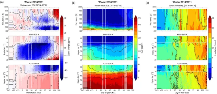
win-Figure 2.Chemical ozone change (left column, in ppmv), assimilated N2O volume mixing ratio (middle column, in ppbv) and the time change of cumulative insolation (right column, in h day−1) during the Arctic winter 2010/11. The top panels of each column represent the vortex mean for each variable (70–90◦N, EQL range) as a function of time and potential temperature. The two panels below show the temporal evolution of the spatial distribution in EQL at selected isentropic surfaces (the mid-stratospheric average between 600 and 800 K and the lower stratospheric average between 425 and 500 K, respectively). The horizontal white solid lines in these plots indicate the EQL of 70◦N, used as the vortex edge border in our study. The shaded areas indicate the temporal gaps in the SMR O3and N2O data sets. The values shown during these periods correspond to the transport model only.
ter. However, in these two cases, the reversal of the zonal-mean zonal wind at 60◦N and 10 hPa, as deduced from the
ECMWF analyses, was shorter than a week, and the polar stratosphere was less disturbed. As we can see in Fig. 1 and Table 1, the observed O3 loss in the mid-stratosphere was
much lower for these less-disturbed winters than for the four above-mentioned events in 2003/04, 2005/06, 2008/09 and 2012/13. The winter 2011/12 was characterised by a minor SSW (no reversal of the zonal wind at 60◦N and 10 hPa
was observed), and in that case the mid-stratospheric loss also overwhelmed the lower stratospheric loss, with a loss ratio comparable to the other four above-mentioned events. Since the mid-stratospheric loss was not greater than 1 ppmv in magnitude, this event was not retained in the composite, but this subjective choice does not affect greatly our results. In the two following sections, we will address separately the cases of the particularly cold and warm Arctic winters, in or-der to further characterise the mechanisms responsible for the chemical ozone destruction in the lower and middle strato-sphere.
4 Lower stratospheric ozone loss during cold winters As described in the introduction (Sect. 1), the ozone loss in the polar lower stratosphere can be explained, to a large extent, by chemical destruction processes involving halogen compounds, occurring in spring when cold vortex air is
ex-posed to sunlight. The Arctic winter 2010/11 is a very good opportunity to study these processes. The zonal-mean zonal wind derived from ECMWF analyses at 55 hPa and 60◦N,
averaged over the two months of February and March 2011, was around 25 m s−1, while the mean for all the years into
consideration in our study is 12.5 m s−1with a standard
de-viation of 5.5 m s−1. This is the only winter for which the
value is above the mean plus 1 standard deviation, which in-dicates a particularly strong and stable vortex. This section is hence dedicated to the study of the O3destruction
mecha-nisms during this specific winter, as an outstanding case of a cold Arctic stratosphere.
Figure 2 shows the temporal evolution of chemical ozone change (left column) and of assimilated N2O volume
mix-ing ratio (middle column) durmix-ing the Arctic winter 2010/11; also shown is the time change of cumulative insolation with a unit of hours per day (right column). The latter was calcu-lated in each model grid box by looking at the solar zenith angle (SZA), and by transporting this information with the advection model. We used a SZA value of 102◦, which is
also known as a border of nautical twilight, as a threshold between day and night. Hence, a local increase of this pa-rameter can indicate both direct exposure of the air parcel to sunlight and mixing with air masses which had received longer insolation.
The top panels of each column represent the vortex mean (70–90◦N, EQL range) for each variable as a function of
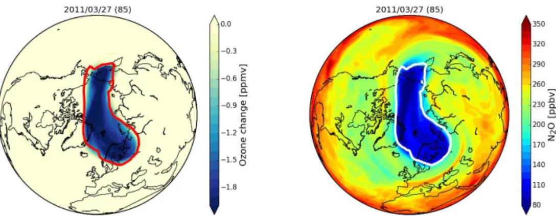
Figure 3.Example of maps of the estimated ozone loss (left panel, in ppmv) and of N2O assimilated fields (right panel, in ppbv). Both maps show the average volume mixing ratio in the lower stratosphere (vertical range 425–500 K) on 27 March 2011, which corresponds to the time and place where the maximum ozone loss occurred. Red and white contour lines indicate the polar vortex border (EQL of 70◦N).
the temporal evolution of the latitudinal distribution in EQL for each variable, averaged over the mid-stratosphere be-tween 600 and 800 K, and the lower stratosphere bebe-tween 425 and 500 K. The white solid lines in these latter plots in-dicate the equivalent latitude of 70◦N, used to delineate the
vortex border. The shaded areas correspond to gaps in the SMR data set. During these periods, the assimilated variables are only transported by the model, with no assimilation incre-ment.
As explained in Sect. 2.1, N2O is commonly used as a
tracer for the transport processes in the stratosphere. The lat-itudinal distribution of N2O is characterised by a very strong
gradient around the EQL of 70◦N, which indicates a
par-ticularly sharp barrier at the vortex edge. We can see that the chemical O3 loss below 500 K was strictly confined to
the interior of the polar vortex, beginning in mid-February. That time corresponds to the end of the polar night, when the vortex air was exposed to solar radiation and the hetero-geneous chemical processes involving halogen compounds could come into effect. The maximum of the vortex-averaged ozone loss (Fig. 2, upper left panel) reached 2.1 ppmv around 450 K by the end of March and early April, when more than 80 % of the ozone was depleted from the stratosphere at that time and altitude. Figure 3 shows maps of the inferred ozone loss and of assimilated N2O averaged over the vertical range
(425–500 K) on 27 March 2011, when the maximum O3loss
was observed. The polar vortex border (EQL of 70◦N),
indi-cated by the thick solid lines, confines the area of ozone loss, which is perfectly consistent with what we see in Fig. 2.
These results are consistent with other studies dedicated to this specific winter, although our estimated loss is slightly lower (approximately 0.4 ppmv) (Arnone et al., 2012; Man-ney et al., 2011; Sinnhuber et al., 2011; Hommel et al., 2014). This is generally the case not only for the Arctic winter in consideration here, but also for other winters and in both hemispheres. Our ozone-loss estimations during the whole time period 2002–2013 have been thoroughly compared to those in other publications in Sagi and Murtagh (2016), and
two plausible explanations for the differences are discussed. One reason is the vortex boundary criterion. Another reason is the instrumental quality such as vertical resolution and sen-sitivity. Considering these issues, we have approximately an uncertainty of 0.2 ppmv in our estimation. The largest differ-ence was found between the O3 loss estimated by
compar-ing SCIAMACHY ozone measurements and quasi-passive ozone calculated by a chemical transport model (Hommel et al., 2014). The corresponding maximum loss is 1 ppmv higher than our result. Quasi-passive ozone is not completely passive but uses an adapted version of the linearised chem-istry scheme excluding heterogeneous chemchem-istry. Thus their quantification only indicates chemical loss by heterogeneous reactions, while ours includes all chemical O3 changes,
in-cluding NOx-induced and even O3production.
As we can see in Fig. 2, the spatial distribution of ozone change in the middle stratosphere (600–800 K) shows a very different pattern to the distribution in the lower stratosphere. The O3 chemical destruction was observed outside the
vor-tex from the beginning of December and extended through the mid-latitude surf zone up to the vortex edge. A maxi-mum loss of approximately 2 ppmv is observed just south of 70◦N of EQL, confined outside of the strong vortex. In
contrast, the loss inside the vortex was below 0.6 ppmv, and began in late January 2011, simultaneously with a short en-hancement in insolation time as seen in the right panel. This increase in insolation time is associated with the weakening and the deformation of the vortex, which now extends into lower latitudes. The polar maps of N2O show that the vortex
was split into two parts by a minor SSW on 4 February 2011 (not shown here). However, the vortex reformed after only a few days. This explains that a slight O3destruction was
ob-served in the vortex during the period following this event, induced by horizontal mixing of NOx-rich air.
In summary, an exceptionally important halogen-induced O3 destruction occurred inside the vortex below 500 K in
lat-Figure 4.Same as Fig. 2 for the composite of the Arctic winters 2003/04, 2005/06, 2008/09 and 2012/13, affected by a mid-winter major sudden stratospheric warming. The time is expressed in days relative to SSW central date.
itudes. The ozone loss during other relatively cold winters, such as 2004/05 and 2007/08, presented similar patterns, al-though the relative magnitudes of losses in the lower and middle stratosphere varied.
5 Mid-stratospheric ozone loss after SSW events We now focus on the chemical ozone destruction in the mid-stratosphere in warm conditions, during the winters 2003/04, 2005/06, 2008/09 and 2012/13. A major midwinter strato-spheric warming is defined as the sudden reversal of the zonal mean zonal wind at a latitude of 60◦ and 10 hPa between
November and March, associated with a positive zonal-mean temperature gradient between 60 and 90◦ at the same
pres-sure level (Andrews et al., 1987). In addition, during these four Arctic winters, the reversal of the zonal-mean zonal wind persisted over more than 1 week according to the ECMWF analyses, which increased the potential of these SSWs to affect the circulation in the middle atmosphere. As already mentioned in Sect. 3, these events were followed by the recovery of the vortex associated with the formation of an elevated stratopause (Orsolini et al., 2010; Pérot et al., 2014). The SSW central date is defined as the first day of the zonal-mean zonal wind reversal at 10 hPa, and has been chosen as a reference date to calculate the composite of these four winters. It corresponds to 4 January 2004, 21 January 2006, 24 January 2009 and 6 January 2013, respectively.
Figure 4 represents the temporal evolution of the chemical ozone change (left column), assimilated N2O volume mixing
ratio (middle column) and the time change of cumulative in-solation (right column) for the composite of warm winters. These winters were characterised by a temperature increase
in the lower stratosphere occurring much earlier than the cli-matological springtime temperature increase associated with the final warming (Sagi and Murtagh, 2016). These warm conditions were not favourable to PSC formation, which ex-plains that the ozone loss in the vertical range 425–500 K is particularly low during these years, as seen by the con-trast with Fig. 2. This loss started from the SSW central date and was confined to the interior of the vortex. The maximum loss in the composite in the lower stratosphere is 0.5 ppmv at 500 K around 15 days after the central date, corresponding to the vortex distortion due to the warming event. This sig-nature is consistent with the loss observed during the Arctic winter 2012/13 using the Aura/MLS instrument by Manney et al. (2015), who explained that moderately cold conditions in December 2012 resulted in extensive PSC formation be-fore the SSW. A combination of early chlorine activation on PSCs and slow chlorine deactivation due to denitrification led to O3loss in January 2013, following the warming event.
These warm winters affected by strong dynamical pertur-bations are however characterised by important ozone loss in the mid-stratosphere. As we can see in Fig. 4 in theθ-range
600–800 K, O3is depleted outside the vortex starting already
in December at low EQL. This ozone depletion expands over a wider range of EQL over the course of the winter, and is not bounded by EQL of 70◦. It reaches the vortex approximately
Figure 5.Ozone loss (top panels, in ppmv) and N2O (bottom panels, in ppbv) maps in the mid-stratosphere (600–800 K) for four selected dates in early 2013. The date format is YYYY/MM/DD. The number of days after the SSW central date (6 January 2013) is given in brackets. Thus, the first map corresponds to the SSW onset, the second one to the break-up of the polar vortex, the third one to the recovery of the vortex, and the last map corresponds to the beginning of the spring.
to ozone production. This is in contrast with PT levels below 500 K, where the vortex air exposure to sunlight-induced O3
destruction due to heterogeneous activation of chlorine. Af-ter the brief production period, a particularly strong chemical ozone loss is observed at high equivalent latitudes, extending from 600 to near 900 K, as there is mixing between vortex air and NOx-rich air from lower latitudes over a broad alti-tude range. This horizontal mixing is visible in the middle panel of Fig. 4, representing the temporal evolution of the N2O spatial distribution. This loss is stronger higher up in
late January and descends down to 600 K, where it signifi-cantly increases up to its maximum around 90 days after the central date. The beginning of the period corresponding to an ozone loss higher than 1.5 ppmv coincides with the vor-tex recovery. As explained in Sect. 1, downward transport of NOx produced by energetic particle precipitation in the mesosphere–lower thermosphere region during winter is an-other source of stratospheric NOx. This is especially true in the case of a winter affected by a SSW-ES event, when this descent motion starts higher than usual and can thus bring more NO down from the mesosphere (Orsolini et al., 2010; Pérot et al., 2014). We therefore expect to see an impact of EPP-NOxon ozone in the middle stratosphere sometime af-ter the warming event. However, we were not able to distin-guish this effect from the impact of the horizontal mixing of air masses in the framework of our study, because it was not possible to assimilate SMR NO observations.
In order to describe in more detail the NOx-induced ozone loss in the case of a warm winter, we look now specifically at O3 loss and N2O polar maps averaged between 600 and
800 K for 4 selected days after the onset of the SSW in Arc-tic winter 2012/13 (Fig. 5). At the beginning, the vortex was
elongated and displaced from the pole, and the O3chemical
loss was observed only outside the vortex (left column). Soon after the central date, the vortex was split into several smaller vortices (second column), and the vortex air was mixed with air parcels from lower latitudes. After the recovery, the O3
destruction occurred mainly inside the vortex (third column). The chemical loss progressively increased and moved to-wards the pole as the NOx-rich air was transported into the vortex, with a maximum at the end of March, as seen in the right column. At that time, there could also be a possible ef-fect of the EPP-NOxtransported downwards in the vortex.
The vortex was sustained even after the end of the polar night, which is consistent with the findings of Thiéblemont et al. (2013) who showed that, when a strong SSW occurs, the final warming tends to occur later than in other years. The inferred ozone loss was at least 2 ppmv by the time of the final warming.
The composite represented in Fig. 4 shows a good sim-ilarity in the vertical and horizontal distribution of chemi-cal ozone change with the case study of the winter 2002/03 discussed in Konopka et al. (2007) (see in particular the Figs. 2 and 3 in this article). As explained in the introduction (Sect. 1), NOx-induced chemical reactions leading to O3 de-pletion play an important role in the altitude range in consid-eration here. The study of the composite of these four winters show that this O3loss mechanism becomes predominant in
6 Conclusions
We assessed the chemical ozone loss in the Northern Hemi-sphere in order to document the inter-annual variability of halogen-induced loss occurring in the lower stratosphere in comparison to the loss in the mid-stratosphere, mainly due to chemical reactions involving NOx species. We applied a data assimilation approach based on an extended version of the off-line wind-driven isentropic transport and assimila-tion model DIAMOND, in which cross-isentropic transport was implemented using diabatic heating rates. Ozone verti-cal profiles retrieved from the emission line at 544 GHz ob-served by Odin/SMR were assimilated into the DIAMOND model in order to obtain spatial and temporal ozone distri-butions at potential temperatures between 425 and 950 K in the Northern Hemisphere. Assimilation experiments of SMR ozone measurements were performed for each Arctic winter between 2001 and 2013. The analysis period for each assimi-lation experiment runs from 1 December to 30 April. Inferred chemical ozone loss was calculated by subtraction of pas-sive ozone, which corresponds to paspas-sively transported ozone fields by DIAMOND model, from the assimilated (or active) ozone. The Arctic ozone losses both in the lower and mid-stratosphere are characterised by a large inter-annual vari-ability.
To describe the ClOx-induced ozone loss in the case of cold winters, we chose to focus on the 2010/11 winter, when the vortex was exceptionally strong in February and March. The sharp vortex barrier during this winter, seen in Fig. 2, allowed a confined ozone depletion to occur in the lower stratosphere below 500 K, with a maximum loss of 2.1 ppmv (0.2 ppmv uncertainty) at 450 K on 27 March 2011. On the other hand, the ozone loss in the middle stratosphere (600–800 K) remained low due to limited horizontal mix-ing into the strong vortex. Similar tendencies are also seen in the other relatively cold winters, such as 2004/05 and 2007/08. Note that during these cold winters, the loss ratio
1OLower3 /1OMiddle3 was greater than 1 (see Table 1).
Konopka et al. (2007) showed, in a case study of the 2002/03 winter affected by a SSW, that NOx-induced loss was comparable to or could even outweigh ClOx-induced loss (albeit at different heights), and was mostly due to meridional transport of NOx-rich air from lower latitudes. Here we have re-assessed and quantified these conclusions over a much longer period, spanning more than a decade characterised by a series of major SSWs. Pronounced mid-stratospheric ozone losses are consistent with occurrences of such major SSW events and their attendant large transport from lower latitudes, as revealed in a composite of the four winters 2003/04, 2005/06, 2008/09 and 2012/13. This loss begins at high altitudes in late January and then descends down to 600 K. Inferred loss of more than 1.5 ppmv between 600–800 K occurs with the vortex recovery in all four win-ters selected for the composite analysis. During these four events, the contribution of the NOx-induced loss was even
more pronounced – broadly by a factor 2 – than during the warming considered in Konopka et al. (2007). The longer du-ration of the zonal wind reversal, as explained in Sect. 3, and the resulting larger disruption of the polar stratosphere, can explain this significant difference.
As shown in this article, ozone depletion in both the lower and middle Arctic stratosphere are significantly influenced by dynamical and thermal conditions. Meanwhile, it is ex-pected that EPP indirectly affects the stratospheric ozone during the polar winter. This is especially true in the South-ern Hemisphere, where Fytterer et al. (2015) indicated con-tributions of EPP-NOxon the Antarctic ozone depletion be-tween 2005 and 2010. Based on the measurements from three satellite instruments, they brought an negative O3
sig-nal out, associated with geomagnetic activity, reaching am-plitudes between−5 and−10 % of the respective O3
back-ground. However, according to Konopka et al. (2007), in the 2002/03 Arctic winter, the NOxdescent from the meso-sphere had a minor impact upon the stratospheric ozone de-pletion in comparison to the meridional transport, as the mesospheric NOx did not propagate low enough to reach the mid-stratosphere. While the warm winters considered in this study, i.e. 2003/04, 2005/06, 2008/09 and 2012/13, were characterised by a strong mesospheric descent (Pérot et al., 2014), we could not find clear evidence that it played a sig-nificant role in the mid-stratospheric ozone depletion. This is partly due to the insufficient temporal sampling of NO ob-servations by the SMR instrument for an assimilation study. Furthermore, assimilation of NOxwould require the develop-ment of a model with relevant stratospheric chemistry. Such investigations would be necessary in order to quantify the small contribution of the downward transport of EPP-NOx from the contribution of horizontal transport of NOx from lower latitudes.
7 Data availability
The DIAMOND assimilation model can be obtained on request to Donal Murtagh (murtagh@chalmers.se). The Odin/SMR level 2 products used in this study are the ver-sion 2.3 of frequency mode 1 (mode ID name: SM_AC2ab) for N2O and frequency mode 2 (mode ID name: SM_AC1e)
for O3. The information needed to access these data sets is
available on http://odin.rss.chalmers.se. The diabatic heating rates, derived from the SLIMCAT model, have been provided by Martyn Chipperfield and Wuhu Feng from the University of Leeds (m.chipperfield@leeds.ac.uk).
Research Council of Norway/CoE under contract 223252/F50. We thank the study group for the added value of chemical data assimilation in the stratosphere and upper troposphere supported by the International Space Science Institute (ISSI). We thank Martyn Chipperfield and Wuhu Feng from the University of Leeds for providing the diabatic heating rates for this study.
Edited by: F. Khosrawi
Reviewed by: two anonymous referees
References
Andrews, D. G., Holton, J. R., and Leovy, C. B.: Middle atmosphere dynamics, Academic Press, New York, NY, USA, 1987. Arnone, E., Castelli, E., Papandrea, E., Carlotti, M., and Dinelli,
B. M.: Extreme ozone depletion in the 2010–2011 Arctic win-ter stratosphere as observed by MIPAS/ENVISAT using a 2-D tomographic approach, Atmos. Chem. Phys., 12, 9149–9165, doi:10.5194/acp-12-9149-2012, 2012.
Bailey, S. M., Thurairajah, B., Randall, C. E., Holt, L., Siskind, D. E., Harvey, V. L., Venkataramani, K., Hervig, M. E., Rong, P., and Russell, J. M.: A multi tracer analysis of thermo-sphere to stratothermo-sphere descent triggered by the 2013 Strato-spheric Sudden Warming, Geophys. Res. Lett., 41, 5216–5222, doi:10.1002/2014GL059860, 2014.
Barth, C. A.: Global observations of nitric oxide in the thermosphere, J. Geophys. Res., 108, 1027, doi:10.1029/2002JA009458, 2003.
Brasseur, G. P. and Solomon, S.: Aeronomy of the Middle Atmo-sphere, Chemistry and Physics of the Stratosphere and Meso-sphere, Vol. 32 of Atmospheric and Oceanographic Sciences Li-brary, Springer, Dordrecht, the Netherlands, 2005.
Charlton, A. J. and Polvani, L. M.: A New Look at Stratospheric Sudden Warmings. Part I: Climatology and Modeling Bench-marks, J. Climate, 20, 449–469, doi:10.1175/JCLI3996.1, 2007. Chipperfield, M. P.: New version of the TOMCAT/SLIMCAT off-line chemical transport model: Intercomparison of stratospheric tracer experiments, Q. J. Roy. Meteor. Soc., 132, 1179–1203, doi:10.1256/qj.05.51, 2006.
El Amraoui, L., Semane, N., Peuch, V. H., and Santee, M. L.: Inves-tigation of dynamical processes in the polar stratospheric vortex during the unusually cold winter 2004/2005, Geophys. Res. Lett., 35, L03803, doi:10.1029/2007GL031251, 2008.
Farman, J. C., Gardiner, B. G., and Shanklin, J. D.: Large losses of total ozone in Antarctica reveal seasonal ClOx/NOxinteraction, Nature, 315, 207–210, doi:10.1038/315207a0, 1985.
Funke, B., López-Puertas, M., Stiller, G. P., and von Clarmann, T.: Mesospheric and stratospheric NOy produced by energetic par-ticle precipitation during 2002–2012, J. Geophys. Res.-Atmos., 119, 4429–4446, doi:10.1002/2013JD021404, 2014.
Fytterer, T., Mlynczak, M. G., Nieder, H., Pérot, K., Sinnhuber, M., Stiller, G., and Urban, J.: Energetic particle induced intra-seasonal variability of ozone inside the Antarctic polar vortex observed in satellite data, Atmos. Chem. Phys., 15, 3327–3338, doi:10.5194/acp-15-3327-2015, 2015.
Grooß, J. U. and Müller, R.: Simulation of ozone loss in Arctic winter 2004/2005, Geophys. Res. Lett., 34, L05804, doi:10.1029/2006GL028901,2007.
Hommel, R., Eichmann, K.-U., Aschmann, J., Bramstedt, K., We-ber, M., von Savigny, C., Richter, A., Rozanov, A., Wittrock, F., Khosrawi, F., Bauer, R., and Burrows, J. P.: Chemical ozone loss and ozone mini-hole event during the Arctic winter 2010/2011 as observed by SCIAMACHY and GOME-2, Atmos. Chem. Phys., 14, 3247–3276, doi:10.5194/acp-14-3247-2014, 2014.
Hurwitz, M. M., Newman, P. A., and Garfinkel, C. I.: The Arctic vortex in March 2011: a dynamical perspective, Atmos. Chem. Phys., 11, 11447–11453, doi:10.5194/acp-11-11447-2011, 2011. Isaksen, I. S. A., Zerefos, C., Wang, W.-C., Balis, D., Eleftheratos, K., Rognerud, B., Stordal, F., Berntsen, T. K., LaCasce, J. H., Søvde, O. A., Olivié, D., Orsolini, Y. J., Zyrichidou, I., Prather, M., and Tuinder, O. N. E.: Attribution of the Arctic ozone col-umn deficit in March 2011, Geophys. Res. Lett., 39, L24810, doi:10.1029/2012GL053876, 2012.
Jackson, D. R. and Orsolini, Y. J.: Estimation of Arctic ozone loss in winter 2004/05 based on assimilation of EOS MLS and SBUV/2 observations, Q. J. Roy. Meteor. Soc., 134, 1833–1841, doi:10.1002/qj.316, 2008.
Jin, J. J., Semeniuk, K., Manney, G. L., Jonsson, A. I., Bea-gley, S. R., McConnell, J. C., Dufour, G., Nassar, R., Boone, C. D., Walker, K. A., Bernath, P. F., and Rinsland, C. P.: Severe Arctic ozone loss in the winter 2004/2005: obser-vations from ACE-FTS, Geophys. Res. Lett., 33, L15801, doi:10.1029/2006GL026752, 2006.
Jones, A., Urban, J., Murtagh, D. P., Eriksson, P., Brohede, S., Ha-ley, C., Degenstein, D., Bourassa, A., von Savigny, C., Sonkaew, T., Rozanov, A., Bovensmann, H., and Burrows, J.: Evolution of stratospheric ozone and water vapour time series studied with satellite measurements, Atmos. Chem. Phys., 9, 6055–6075, doi:10.5194/acp-9-6055-2009, 2009.
Khosrawi, F., Urban, J., Pitts, M. C., Voelger, P., Achtert, P., San-tee, M. L., Manney, G. L., and Murtagh, D.: Denitrification and polar stratospheric cloud formation during the Arctic win-ter 2009/2010 and 2010/2011 in comparison, in: Proceedings of the ESA Atmospheric Science Conference 18–22 June 2012, Eur. Space Agency Spec. Publ., Bruges, Belgium, 2012.
Konopka, P., Engel, A., Funke, B., Müller, R., Grooß, J.-U., Günther, G., Wetter, T., Stiller, G., von Clarmann, T., Glatthor, N., Oelhaf, H., Wetzel, G., López-Puertas, M., Pirre, M., Huret, N., and Riese, M.: Ozone loss driven by nitro-gen oxides and triggered by stratospheric warmings can out-weigh the effect of halogens, J. Geophys. Res., 112, D05105, doi:10.1029/2006JD007064, 2007.
Kuttippurath, J., Godin-Beekmann, S., Lefèvre, F., and Pazmiño, A.: Ozone depletion in the Arctic winter 2007–2008, Int. J. Re-mote Sens., 30, 4071–4082, doi:10.1080/01431160902821965, 2009.
Kuttippurath, J., Godin-Beekmann, S., Lefèvre, F., and Goutail, F.: Spatial, temporal, and vertical variability of polar stratospheric ozone loss in the Arctic winters 2004/2005–2009/2010, Atmos. Chem. Phys., 10, 9915–9930, doi:10.5194/acp-10-9915-2010, 2010.
Lambert, A., Read, W. G., Livesey, N. J., Santee, M. L., Manney, G. L., Froidevaux, L., Wu, D. L., Schwartz, M. J., Pumphrey, H. C., Jimenez, C., Nedoluha, G. E., Cofield, R. E., Cuddy, D. T., Daffer, W. H., Drouin, B. J., Fuller, R. A., Jarnot, R. F., Knosp, B. W., Pickett, H. M., Perun, V. S., Snyder, W. V., Stek, P. C., Thurstans, R. P., Wagner, P. A., Waters, J. W., Jucks, K. W., Toon, G. C., Stachnik, R. A., Bernath, P. F., Boone, C. D., Walker, K. A., Urban, J., Murtagh, D., Elkins, J. W., and Atlas, E.: Vali-dation of the Aura Microwave Limb Sounder middle atmosphere water vapor and nitrous oxide measurements, J. Geophys. Res., 112, D24S36, doi:10.1029/2007JD008724, 2007.
Manney, G. L., Santee, M. L., Froidevaux, L., Hoppel, K., Livesey, N. J., and Waters, J. W.: EOS MLS observations of ozone loss in the 2004–2005 Arctic winter, Geophys. Res. Lett., 33, L04802, doi:10.1029/2005GL024494, 2006.
Manney, G. L., Santee, M. L., Rex, M., Livesey, N. J., Pitts, M. C., Veefkind, P., Nash, E. R., Wohltmann, I., Lehmann, R., Froide-vaux, L., Poole, L. R., Schoeberl, M. R., Haffner, D. P., Davies, J., Dorokhov, V., Gernandt, H., Johnson, B., Kivi, R., Kyro, E., Larsen, N., Levelt, P. F., Makshtas, A., McElroy, C. T., Nakajima, H., Parrondo, M. C., Tarasick, D. W., von der Gathen, P., Walker, K. A., and Zinoviev, N. S.: Unprecedented Arctic ozone loss in 2011, Nature, 478, 469–475, doi:10.1038/nature10556, 2011. Manney, G. L., Lawrence, Z. D., Santee, M. L., Livesey, N. J.,
Lam-bert, A., and Pitts, M. C.: Polar processing in a split vortex: Arctic ozone loss in early winter 2012/2013, Atmos. Chem. Phys., 15, 5381–5403, doi:10.5194/acp-15-5381-2015, 2015.
Ménard, R. and Chang, L.-P.: Assimilation of Stratospheric Chem-ical Tracer Observations Using a Kalman Filter. Part II: χ2 -Validated Results and Analysis of Variance and Correlation Dy-namics, Mon. Weather Rev., 128, 2672–2686, doi:10.1175/1520-0493(2000)128<2672:AOSCTO>2.0.CO;2, 2000.
Ménard, R., Cohn, S. E., Chang, L.-P., and Lyster, P. M.: Assimila-tion of stratospheric chemical tracer observaAssimila-tions using a Kalman filter. Part I: Formulation, Mon. Weather Rev., 128, 2654–2671, doi:10.1175/1520-0493(2000)128<2654:AOSCTO>2.0.CO;2, 2000.
Murtagh, D., Frisk, U., Merino, F., Ridal, M., Jonsson, A., Stegman, J., Witt, G., Eriksson, P., Jiménez, C., Megie, G., de la Noë, J., Ricaud, P., Baron, P., Pardo, J. R., Hauchcorne, A., Llewellyn, E. J., Degenstein, D. A., Gattinger, R. L., Lloyd, N. D., Evans, W. F. J., McDade, I. C., Haley, C. S., Sioris, C., von Savigny, C., Solheim, B. H., McConnell, J. C., Strong, K., Richardson, E. H., Leppelmeier, G. W., Kyrölä, E., Auvinen, H., and Oikarinen, L.: An overview of the Odin atmospheric mission, Can. J. Phys., 80, 309–319, doi:10.1139/p01-157, 2002.
Nash, E. R., Newman, P. A., Rosenfield, J. E., and Schoeberl, M. R.: An objective determination of the polar vortex using Ertel’s potential vorticity, J. Geophys. Res., 101, 9471–9478, doi:10.1029/96JD00066, 1996.
Orsolini, Y. J., Urban, J., Murtagh, D. P., Lossow, S., and Limpa-suvan, V.: Descent from the polar mesosphere and anomalously high stratopause observed in 8 years of water vapor and tempera-ture satellite observations by the Odin Sub-Millimeter Radiome-ter, J. Geophys. Res., 115, D12305, doi:10.1029/2009JD013501, 2010.
Pérot, K., Urban, J., and Murtagh, D. P.: Unusually strong nitric oxide descent in the Arctic middle atmosphere in early 2013 as
observed by Odin/SMR, Atmos. Chem. Phys., 14, 8009–8015, doi:10.5194/acp-14-8009-2014, 2014.
Prather, M. J.: Numerical Advection by Conservation of Second-Order Moments, J. Geophys. Res., 91, 6671–6681, doi:10.1029/JD091iD06p06671, 1986.
Randall, C. E.: Stratospheric effects of energetic particle pre-cipitation in 2003–2004, Geophys. Res. Lett., 32, L05802, doi:10.1029/2004GL022003, 2005.
Rex, M., Salawitch, R. J., Deckelmann, H., von der Gathen, P., Harris, N. R. P., Chipperfield, M. P., Naujokat, B., Reimer, E., Allaart, M., Andersen, S. B., Bevilacqua, R., Braathen, G. O., Claude, H., Davies, J., De Backer, H., Dier, H., Dorokov, V., Fast, H., Gerding, M., Hoppel, K., Johnson, B., Kyrö, E., Lityn-ska, Z., Moore, D., Nagai, T., Parrondo, M. C., Risley, D., Skrivankova, P., Stübi, R., Trepte, C., Viatte, P., and Zerefos, C.: Arctic winter 2005: Implications for stratospheric ozone loss and climate change, Geophys. Res. Lett., 33, L23808, doi:10.1029/2006GL026731, 2006.
Rösevall, J. D., Murtagh, D. P., and Urban, J.: Ozone depletion in the 2006/2007 Arctic winter, Geophys. Res. Lett., 34, L21809, doi:10.1029/2007GL030620, 2007a.
Rösevall, J. D., Murtagh, D. P., Urban, J., and Jones, A. K.: A study of polar ozone depletion based on sequential assimilation of satellite data from the ENVISAT/MIPAS and Odin/SMR in-struments, Atmos. Chem. Phys., 7, 899–911, doi:10.5194/acp-7-899-2007, 2007b.
Rösevall, J. D., Murtagh, D. P., Urban, J., Feng, W., Eriksson, P., and Brohede, S.: A study of ozone depletion in the 2004/2005 Arctic winter based on data from Odin/SMR and Aura/MLS, J. Geophys. Res., 113, D13301, doi:10.1029/2007JD009560, 2008. Sagi, K. and Murtagh, D.: A long term study of polar ozone loss derived from data assimilation of Odin/SMR observations, At-mos. Chem. Phys. Discuss., doi:10.5194/acp-2016-352, in re-view, 2016.
Sagi, K., Murtagh, D., Urban, J., Sagawa, H., and Kasai, Y.: The use of SMILES data to study ozone loss in the Arctic win-ter 2009/2010 and comparison with Odin/SMR data using as-similation techniques, Atmos. Chem. Phys., 14, 12855–12869, doi:10.5194/acp-14-12855-2014, 2014.
Singleton, C. S., Randall, C. E., Harvey, V. L., Chipperfield, M. P., Feng, W., Manney, G. L., Froidevaux, L., Boone, C. D., Bernath, P. F., Walker, K. A., McElroy, C. T., and Hoppel, K. W.: Quanti-fying Arctic ozone loss during the 2004–2005 winter using satel-lite observations and a chemical transport model, J. Geophys. Res., 112, D07304, doi:10.1029/2006JD007463, 2007.
Sinnhuber, B. M., Stiller, G., Ruhnke, R., von Clarmann, T., Kellmann, S., and Aschmann, J.: Arctic winter 2010/2011 at the brink of an ozone hole, Geophys. Res. Lett., 38, L24814, doi:10.1029/2011GL049784, 2011.
Solomon, S., Ivy, D. J., Kinnison, D., Mills, M. J., Neely, R. R., and Schmidt, A.: Emergence of healing in the Antarctic ozone layer, Science, 353, 269–274, doi:10.1126/science.aae0061, 2016. Sonkaew, T., von Savigny, C., Eichmann, K.-U., Weber, M.,
Søvde, O. A., Orsolini, Y. J., Jackson, D. R., Stordal, F., Isaksen, I. S. A., and Rognerud, B.: Estimation of Arctic O3loss during winter 2006/2007 using data assimilation and comparison with a chemical transport model, Q. J. Roy. Meteor. Soc., 137, 118–128, doi:10.1002/qj.740, 2011.
Strong, K., Wolff, M. A., Kerzenmacher, T. E., Walker, K. A., Bernath, P. F., Blumenstock, T., Boone, C., Catoire, V., Coffey, M., De Mazière, M., Demoulin, P., Duchatelet, P., Dupuy, E., Hannigan, J., Höpfner, M., Glatthor, N., Griffith, D. W. T., Jin, J. J., Jones, N., Jucks, K., Kuellmann, H., Kuttippurath, J., Lam-bert, A., Mahieu, E., McConnell, J. C., Mellqvist, J., Mikuteit, S., Murtagh, D. P., Notholt, J., Piccolo, C., Raspollini, P., Ri-dolfi, M., Robert, C., Schneider, M., Schrems, O., Semeniuk, K., Senten, C., Stiller, G. P., Strandberg, A., Taylor, J., Tétard, C., Toohey, M., Urban, J., Warneke, T., and Wood, S.: Validation of ACE-FTS N2O measurements, Atmos. Chem. Phys., 8, 4759– 4786, doi:10.5194/acp-8-4759-2008, 2008.
Thiéblemont, R., Orsolini, Y. J., Hauchecorne, A., Drouin, M.-A., and Huret, N.: A climatology of frozen-in anticyclones in the spring arctic stratosphere over the period 1960–2011, J. Geo-phys. Res.-Atmos., 118, 1299–1311, doi:10.1002/jgrd.50156, 2013.
Tummon, F., Hassler, B., Harris, N. R. P., Staehelin, J., Steinbrecht, W., Anderson, J., Bodeker, G. E., Bourassa, A., Davis, S. M., Degenstein, D., Frith, S. M., Froidevaux, L., Kyrölä, E., Laine, M., Long, C., Penckwitt, A. A., Sioris, C. E., Rosenlof, K. H., Roth, C., Wang, H.-J., and Wild, J.: Intercomparison of vertically resolved merged satellite ozone data sets: interannual variabil-ity and long-term trends, Atmos. Chem. Phys., 15, 3021–3043, doi:10.5194/acp-15-3021-2015, 2015.
Urban, J., Lautié, N., Le Flochmoën, E., Jiménez, C., Eriksson, P., de La Noë, J., Dupuy, E., Ekström, M., El Amraoui, L., Frisk, U., Murtagh, D., Olberg, M., and Ricaud, P.: Odin/SMR limb observations of stratospheric trace gases: Level 2 processing of ClO, N2O, HNO3, and O3, J. Geophys. Res., 110, D14307, doi:10.1029/2004JD005741, 2005a.
Urban, J., Lautié, N., Le Flochmoën, E., Jiménez, C., Eriksson, P., de La Noë, J., Dupuy, E., El Amraoui, L., Frisk, U., Jé-gou, F., Murtagh, D., Olberg, M., Ricaud, P., Camy-Peyret, C., Dufour, G., Payan, S., Huret, N., Pirre, M., Robinson, A. D., Harris, N. R. P., Bremer, H., Kleinböhl, A., Küllmann, K., Künzi, K., Kuttippurath, J., Ejiri, M. K., Nakajima, H., Sasano, Y., Sugita, T., Yokota, T., Piccolo, C., Raspollini, P., and Ri-dolfi, M.: Odin/SMR limb observations of stratospheric trace gases: Validation of N2O, J. Geophys. Res., 110, D09301, doi:10.1029/2004JD005394, 2005b.