Improvement of semi-analytical design sensitivities of
non-linear structures using equilibrium relations
E. Parente Jr. and L. E. Vaz
∗
;†Civil Engineering Department;PUC-Rio;Rio de Janeiro;RJ;Brazil
SUMMARY
The accuracy problem of the semi-analytical method for shape design sensitivity analysis has been reported for linear and non-linear structures. The source of error is the numerical dierentiation of the element internal force vector, which is inherent to the semi-analytical approach. Such errors occur for structures whose displacement eld is characterized by large rigid body rotations of individual elements. This paper presents a method for the improvement of semi-analytical sensitivities. The method is based on the element free body equilibrium conditions, and on the exact dierentiation of the rigid body modes. The method is ecient, simple to code, and can be applied to linear and non-linear structures. The numerical examples show that this approach eliminates the abnormal errors that occur in the conventional semi-analytical method. Copyright ? 2001 John Wiley & Sons, Ltd.
KEY WORDS: design sensitivity; semi-analytical method; non-linear analysis
1. INTRODUCTION
The most ecient numerical optimization algorithms require the evaluation of design sensi-tivities in order to compute the search direction of the optimization process. The convergence of this process is strongly dependent on the quality of the design sensitivity. Moreover, the sensitivity analysis is generally a very time-consuming task. Therefore, the ecient and accu-rate computation of the design sensitivities plays a central role in the overall eciency of the shape optimization process. The existing methods for performing design sensitivity analysis are the global nite dierence method, the analytical method and the semi-analytical method. The implementation of the global nite dierence method is simple and independent of the type of nite element. On the other hand, this method is not computationally ecient, specially for non-linear structures. Moreover, the accuracy of this method is strongly dependent on the perturbation size of the design variable.
∗Correspondence to: L. E. Vaz, Civil Engineering Department, PUC-Rio, Marques de S˜ao Vicente 225, 22453-900,
Rio de Janeiro, RJ, Brazil
†E-mail: [email protected]
Contract=grant sponsor: CNPq Brazilian Research Agency
The analytical method is computationally ecient and reliable, since the problem of the choice of the perturbation size does not need to be addressed. However, its formulation and implementation are more dicult and dependent on the particular nite element type. This method has been successfully applied to isoparametric and truss elements [1–3], but its application to more complex elements can be very cumbersome, specially for non-linear structures.
The semi-analytical (SA) method combines the eciency of the analytical method with the simplicity and the generality of the global nite dierence method. Nevertheless, it has been reported that this method can lead to severe errors in certain cases. It has been shown that such errors occur when the displacement eld is dominated by the rigid body rotations of individual elements. This behaviour occurs in linear [4–6] as well as non-linear [3] structures. The computation of the displacement sensitivities by the analytical and semi-analytical methods involves the evaluation of the global pseudo-load vector. This vector is computed by the dierentiation of the element internal force vector w.r.t. the design variables. In the conventional semi-analytical method, these derivatives are usually evaluated by means of the forward nite dierence scheme. This procedure has been recognized as the source of errors in the semi-analytical method [4–6]. Three dierent approaches have been proposed to solve this problem.
The rst one applies higher-order nite dierence schemes (e.g. central dierence) to the numerical dierentiation. Its implementation for linear and non-linear structures is simple and general. However, this approach can lead to additional computational eorts.
The second one is called ‘exact’ semi-analytical method [6–8] and uses correction factors to upgrade nite dierences to exact derivatives. This method is not always straightforward to implement, specially for non-linear structures.
The third approach, called rened semi-analytical (RSA) method was initially formulated for linear structures [9; 10]. Later, the method was extended to linear buckling [11] and to geometrically non-linear structures [12–14]. The basic idea of the method is to improve the nite dierence evaluation of the pseudo-load vector using the rigid body motions and their derivatives. The implementation of this method is simple and general since it does not depend on the element formulation but only on the element degrees of freedom. The rigid body modes are obtained using the property that the increment of rigid body displacements do not produce increment of element deformations [12–14].
In the present work, RSA method is developed using a dierent approach. The new approach is based on the free body equilibrium conditions of an individual element. Although both approaches lead to the same nal expressions for the correction of the pseudo-load vector, the new approach allows an easy physical interpretation and a simple determination of the rigid body motions, highlighting the similarities and dierences between the linear and the non-linear cases. The numerical examples presented in this paper, show once again that the RSA method can dramatically reduce the errors presented by the conventional SA method for some non-linear structures.
2. SHAPE SENSITIVITY ANALYSIS
be evaluated in a straightforward manner. Thus, the rst objective of the sensitivity analysis is the computation of the sensitivity of nodal displacements.
Without loss of generality, let us consider a structure described by a single design variableb. The starting point for the displacement sensitivity analysis is the FE non-linear equilibrium equation
g(u; b)−f(b) =0 (1)
where u is the displacement vector, g is the internal force vector, is the load factor, and
f is the reference vector for external loads. It should be noticed that u and are implicit functions of b.
For a xed load factor, the total derivative of Equation (1) w.r.t. b, is
@g @u
du
db+ @g @b−
df
db=0 (2)
Noting that the derivative of internal forces w.r.t. the nodal displacements is the tangent stiness matrix [15] Kt, the sensitivity of the nodal displacement vector can be computed from
Kt du
db=
df
db− @g
@b=pb (3)
where p is known as the pseudo-load vector.
In the above equation, the pseudo-load vector pb is evaluated using the total derivative of the external load vector and the partial derivative of the internal load vector w.r.t. b
(keeping u xed). The derivative of the external load vector is evaluated exactly in the same way as in the linear analysis. As shown in Equation (3), the displacement sensitivities are computed without iteration. In the solution phase, the stiness matrix was factored in the
LDLt form. Thus, only vector reductions and back-substitutions are necessary for sensitivity evaluation.
The global pseudo-load vector is assembled from element vectors in exactly the same way as the internal and the external load vectors. Therefore, the key to the process is the computation of the internal force derivative of each element.
In the semi-analytical method, the derivative of the element internal force vector is evaluated by nite dierences. Using the rst-order forward-dierence scheme, this derivative is given by
dg
db=
g(b+ b)−g(b)
b (4)
where b is the absolute perturbation on the variable b. Since it is dicult to dene a valid perturbation for the entire range of variation of b, the absolute perturbation is generally computed using the equation
b=b (5)
where is a given relative perturbation. The same procedure is applied to the computation of the derivative of the external load vector.
co-ordinates aj by using the chain rule. Thus, the displacement sensitivity w.r.t. bi can be computed from
@u @bi
= @u
@aj
@aj
@bi
(6)
In this equation and in the rest of this paper, the summation convention for repeated indices is used. Alternatively, it can be more ecient to directly compute the displacement sensitivity using Equation (3) with the pseudo-load vector given by
pbi=paj
@aj
@bi
(7)
where
paj=
@f @aj
− @g
@aj
(8)
The derivatives of nodal co-ordinates w.r.t. the design variables are easily evaluated [7], thus we are going to focus on the computation of the sensitivities w.r.t. the nodal co-ordinates.
The derivative of the external load vector can also be accurately evaluated by nite dif-ferences. It can be noted that these derivatives vanish for design independent loads (e.g. concentrated nodal loads). Thus, the source of the abnormal errors that occur in the con-ventional semi-analytical method are the errors in the nite dierence computation of the derivative of the element internal force vector w.r.t. the nodal co-ordinates [3]. The objective of this paper is to present a method to reduce these errors.
3. REFINED SEMI-ANALYTICAL METHOD
It is important to remember that, regardless of the particular element formulation, the in-ternal force vector of each element must satisfy the equilibrium conditions for a free body. Mathematically, these conditions can be represented by the inner product
g·rk= 0 (9)
where rk is a vector that describes the equilibrium conditions. It is well known, from elemen-tary mechanics, that a system of self-equilibrating forces applied to a body does not produce any work when the body is submitted to rigid body displacements. Therefore, the rk vectors can be interpreted physically as the rigid body modes associated to the given nite element. The number of equilibrium equations is independent of the particular element, but it depends on the problem at hand. Thus, for three-dimensional problems, there are three equations for the equilibrium of forces:
PF
x= 0; PFy= 0; PFz= 0 (10)
and three equations for the equilibrium of moments:
PM
x= 0; PMy= 0; PMz= 0 (11)
be shown that the dierentiation of Equation (9) w.r.t. the nodal displacements yield
Krk=0 (12)
It can be realized that the vectorsrk form a basis for a vector space. For the purposes of this work, these basis vectors should be mutually orthogonal (ri·rj= 0 fori6=j), but not unitary. As it will be shown later, these vectors are explicit functions of the nodal co-ordinates, and can be easily dierentiated in an exact manner.
The dierentiation of Equation (9) w.r.t. aj yields
g′·r
k+g·r′k= 0 (13)
where, in this equation and in the rest of this paper, g′ denotes @g=@a
j and so on. Clearly, the internal force derivative computed by the analytical method satises the Equation (13) for the equilibrium of forces and moments. On the other hand, numerical experiments carried out by the authors showed that the semi-analytical derivatives satisfy this condition only for the equilibrium of forces, and that the errors in moment equations are critical for problems in which the displacement eld is characterized by large rigid body rotations of individual elements. In the present paper, Equation (13) is used as the starting point of the method for improving semi-analytical sensitivities.
Omitting the subscripts aj for the pseudo-load vector, Equation (8) can be written as
p=f′−g′ (14)
Decomposing the vector g′ in a component in the space spanned byr
k and another component orthogonal to this space, the derivative of the element internal force vector can be written as
g′= g′·rk
rk·rk
rk+
g′− g′·rk
rk·rk
rk
(15)
Now, the substitution of (15) in (14) yields
p=f′−g′+ g′·rk
rk·rk
rk−
g′·r k
rk·rk
rk (16)
The fourth term on the right-hand side of the equation above represents the projection of
g′ along r
k, which is inaccurately evaluated by nite dierences, specially when large rigid body rotations are present. On the other hand, the second and third terms together represent the component of g′ orthogonal to the space spanned by r
k, which is less sensitive to the errors in the evaluation of g′.
It should be noted, from Equation (13), that
g′·r
k= −g·rk′ (17)
This means that the projection of g′ along r
k can be evaluated in an exact manner, since the derivative of rk can be exactly computed. This procedure can dramatically decrease the abnormal errors in the computation of the pseudo-load vector when large rigid body rotations are present.
Using Equation (17), the pseudo-load vector can be written as
p=f′−g′+ g′·rk
rk·rk
rk+
g·r′ k
rk·rk
but in the practical implementation of the method it is more ecient to use the expression
p=f′−g′+
krk (19)
where
k=
g′·r
k+g·r′k
rk·rk
(20)
Obviously, the parameters k of Equation (13) are zero for analytical derivatives. Therefore, this condition can be used as a test for the implementation of the analytical method of sensitivity analysis for a particular nite element.
From the equations above, it can be noted that the objective of the present method is to replace the components of g′ in the direction of r
k, which are inaccurately evaluated by nite dierences, by its analytical derivative, which can be easily computed. It should be emphasized that this method is completely independent of a particular element formulation, and can be implemented in a generic form. Moreover, it can be applied to linear and non-linear structures. The approach used in this work gives an interesting interpretation of the RSA method. From Equation (18), the rened sensitivity of the internal force vector can be written as
g′
ref=g′− g′·r
k+g·rk′
rk·rk
rk (21)
The dot product of g′
ref by the rk vector leads to
g′
ref·rk=g′·rk−
g′·r
k+g·r′k
rk·rk
rk·rk=g′·rk−(g′·rk+g·r′k) = −g·r′k (22)
Finally, rearranging the terms, the following expression is obtained:
g′
ref·rk+g·rk′= 0 (23)
This expression shows that the rened sensitivity of the internal force vector satises exactly the orthogonality conditions given by expression (13), even when the sensitivity of this vector is not well evaluated by nite dierences. Therefore, the RSA method corrects the sensitivity of the internal force vector in order to satisfy the orthogonality conditions derived from the free body equilibrium equations of an individual element.
4. IMPLEMENTATION ASPECTS
In order to compute the pseudo-load vector using Equations (19) and (20), it is necessary to compute the orthogonal basis vector rk and the respective derivatives r′k. To this purpose, the rst step is to compute a set of non-orthogonal basis vectors rk and the respective derivatives
r′
k. After that, an orthogonalization procedure is applied to these vectors yielding the desired vectors rk and rk′ [10].
4.1. Non-orthogonal basis vectors
d.o.f. are translations. Therefore, the internal force vector is composed only by forces. For elements that also have rotations as d.o.f., the internal force vector is composed by forces and moments.
The rst basis vectors express the equilibrium of forces in each global direction (x; y; z), and are given by
r1 r2 r3 =
F1 F2 · · · Fn (24)
where n is the number of element nodes, and
Fi=
1 0 0
0 1 0
0 0 1
(25)
It is interesting to note that these basis vectors are not a function of the element nodal coordinates. Therefore,
r′
k=0; for k63 (26)
The other basis vectors express the equilibrium of moments around each global axis (x; y; z), and are given by
r4 r5 r6 =
M1 M2 · · · Mn (27)
In this equation, each sub-matrix is given by
Mi=
0 −(zi+wi) (yi+vi) (zi+wi) 0 −(xi+ui) −(yi+vi) (xi+ui) 0
(28)
where (xi; yi; zi) are the element nodal coordinates, and (ui; vi; wi) are the element nodal dis-placements. The nodal displacements are included in the equation above since the equilibrium for geometrically non-linear structures must be written in the deformed conguration.
In order to apply this method to linear or to pure materially non-linear structures, the nodal displacements should be discarded as the equilibrium is written in the undeformed conguration. Thus, Equation (28) is rewritten as
Mi=
0 −zi yi
zi 0 −xi −yi xi 0
(29)
The partial derivative of the sub-matrix Mi w.r.t the nodal coordinate aj is given by
@Mi @aj =
0 0 0
0 0 −1
0 1 0
and
@Mi
@aj
=0 for j6=i (31)
The derivatives for aj=yi and for aj=zi are completely analogous and will not be shown here.
4.2. Orthogonalization procedure
Using the Gram–Schmidt orthogonalization procedure [16], the orthogonal basis vectorsrk are computed from the non-orthogonal vectors rk by the equation
rk= rk− k−1
P
p=1
apkrp (32)
where
apk =rk·rp
rp·rp
(33)
Since the rst three vectors rk are already mutually orthogonal, the application of this proce-dure yields
rk= rk for k63 (34)
The derivative of orthogonal basis vectors rk is given by
r′ k= r′k−
k−1 P
p=1
apk′rp+apkr′p
(35)
In order to compute this derivative exactly, it is necessary to compute the terms apk′. However, in the present method, the vectors r′
k are used only to compute the product g·r′k, which is given by
g·r′
k=g·r′k− k−1
P
p=1
apk′g·rp+apkg·r′p
(36)
Using the equilibrium condition
g·rp= 0 (37)
Equation (36) can be simplied to
g·r′
k=g·r′k− k−1
P
p=1 apkg·r′
p (38)
Therefore, in the practical implementation of the present method, the vectors r′
k can be computed using
r′
k:= r′k− k−1
P
p=1 apkr′
p (39)
From Equations (34) and (26), it can be observed that
r′
Since the vectors associated to force equilibrium are always independent of the nodal co-ordinates and mutually orthogonal, Equations (26) and (34) are valid for all element types, and only the number of these vectors is dependent on the element at hand. It is important to underline that the structure of (32) is identical to the structure of (39); thus, the vectors rk and r′
k can be handled in the same way in the orthogonalization procedure. Finally, it can be seen from the equations above that the orthogonalization procedure is independent from nite element type and can be implemented in a generic way.
4.3. Computer implementation
The presented method was implemented in the FEMOOP program [17] developed in the Civil Engineering Department of the Pontical Catholic University of Rio de Janeiro (PUC-Rio). This program is written in C++ language and uses the concepts of Object Oriented Programming (OOP) to build an easily extendable framework for computational mechanics.
In this program, an object of the Element class contains pointers to Analysis Model and
Shape classes. The former is responsible for the specic features of the type of analysis being
performed (e.g. truss, plane stress, plate, shell, solid, etc.) and the latter holds the geometric and eld interpolation aspects of an element (e.g. Q4, Q8, T6, BRICK8, BRICK20, TET10, etc.). Using these classes, it is possible to treat dierent element types in an unied way. This approach is particularly elegant in the case of isoparametric elements.
In the FEMOOP program, the non-orthogonal basis vectors and their derivatives are evalu-ated by a virtual method dened for each Analysis Modelsub-class. Therefore, this method is valid for all nite element shapes associated with the given model. Since the orthogonalization process does not depend on Shape and Analysis Model classes, it is performed by a specic method of the Element class. It is important to note that the Shape and the other classes of the program do not require any modication.
5. NUMERICAL EXAMPLES
This section presents examples to illustrate the eectiveness of the present method to improve the shape sensitivities computed by the semi-analytical method. The rst three examples are truss structures, and the other two are plane stress problems discretized with isoparametric elements. The Total Lagrangian approach [15; 18] is used in the element formulation to deal with the large displacement eects. The load-controlled Newton–Raphson algorithm is used to evaluate the equilibrium points of each example.
The results obtained by the semi-analytical (SA) method for shape sensitivity analysis are compared with the results obtained by the rened semi-analytical method (RSA), presented in this paper. The relative error (e) for each sensitivity (d) is dened as
e=
d−dAM dAM
(41)
Figure 1. Two-bar truss (EA = 105 kN, P= 1 kN, b= 10 m, h= 1 m).
Figure 2. Relative errors for the two-bar truss.
To perform the comparison between the SA and the RSA sensitivities, the relative error is shown as a function of the relative perturbation (). This perturbation is dened as
=s
s (42)
where s is the element length in the perturbation direction. If this length is zero for truss models, then s is the total element length. The concept of boundary layer [7] is used in the examples. Therefore, when the nite element mesh is perturbed, only the elements connected with the boundary nodes are perturbed.
5.1. Two-bar truss
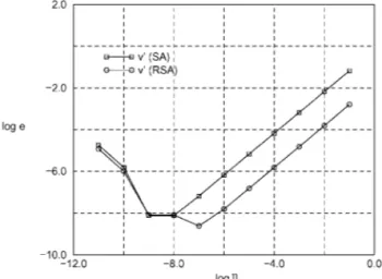
Consider the plane truss shown in Figure 1, where the design variable is the height h of the truss. Due to symmetry conditions, only the vertical displacement v of the central node is considered. The relative errors in the computation of v′ for a load factor (= 75) close to the rst limit point are given in Figure 2.
This structure does not have large rigid body rotations, thus the SA method generates ac-ceptable results for a large range of relative perturbations, as shown in Figure 2. Nevertheless, this gure also shows that the proposed method improves the quality of the SA results for perturbations greater than 10−8, where the sensitivity error is dominated by the truncation
Figure 3. Star-shaped truss (EA = 10976 kN,P= 1 kN).
Figure 4. Relative errors for the star-shaped truss.
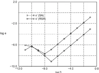
5.2. Star-shaped truss
The second example deals with the hexagonal star-shaped dome depicted in Figure 3. The de-sign variable is the vertical coordinate of the central node. This structure has a highly nonlinear behaviour with several limit points [19]. However, in the present work, the sensitivity of the vertical displacement v of the central node is computed at a load factor (= 3:4) before the rst limit point. The relative errors for this sensitivity are shown in Figure 4.
The displacement eld of this structure is not dominated by the rigid body rotation of individual elements. However, these rotations are greater than the rotations of the elements in the previous example. Therefore, as shown in Figure 4, the SA method provides acceptable results for a large range, but the improvement obtained with the proposed method in this example is greater than the improvement obtained in the previous test case.
It is worth noting that, in the adopted scale, the relative errors for both methods decrease almost linearly with the relative perturbation up to the point where the round-o errors be-come signicant. For relative perturbations smaller than 10−8 the round-o errors become
Figure 5. Cantilever truss (L= 50 m, H= 1 m, EA = 105 kN, and P= 1 kN).
Figure 6. Relative errors for the long-span truss.
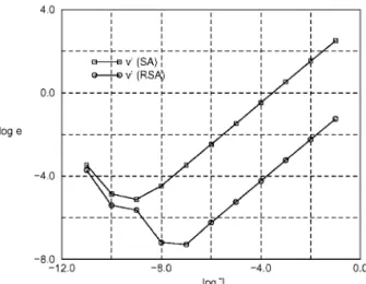
5.3. Cantilever truss
This example deals with the long-span cantilever truss depicted in Figure 5. The structure has 102 nodes, and 251 bars and the design variable is the horizontal co-ordinate (L) of the loaded nodes. It should be noted that, unlike the previous examples, the displacement eld of this structure is dominated by the rigid body rotations of individual elements.
The sensitivity v′ of the vertical displacement of the point A is computed for = 3:0. The relative errors for both methods are given in Figure 6. This gure shows that the SA method does not generate good results in this example. Only for relative perturbations smaller than 10−5, the relative error is smaller than 1 per cent. On the other hand, the proposed method
eliminates these abnormal errors, and very acceptable results are computed for perturbations from 10−4 to 10−10.
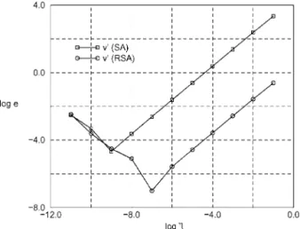
5.4. Cantilever beam
Figure 7. Cantilever beam (E= 2:1×10⁵ N=mm2,= 0:3,P= 1 N=mm,H= 1 mm,L= 50 mm).
Figure 8. Relative errors for the cantilever beam.
The beam is subjected to a load at the free end and is modeled by a regular mesh of 200×4 quadratic isoparametric (8-node) elements, as shown in Figure 7. The numerical integration is carried out with a 2×2 Gaussian integration scheme.
The sensitivities of the vertical displacement of node A are computed for = 7:0. The SA sensitivity errors as a function of the relative perturbations are given in Figure 8. From this gure, one can observe that the conventional SA method provides inaccurate results for almost the entire range of relative perturbations.
The benets of the proposed method become very signicant in this example. It can be seen from Figure 8 that the errors of the sensitivities computed using this method, for a large range of relative perturbations, is approximately 100 times smaller than the errors of the conventional SA method. As in previous examples, for very small perturbations, the round-o errors are dominant and the proposed method gives approximately the same results as the conventional SA method.
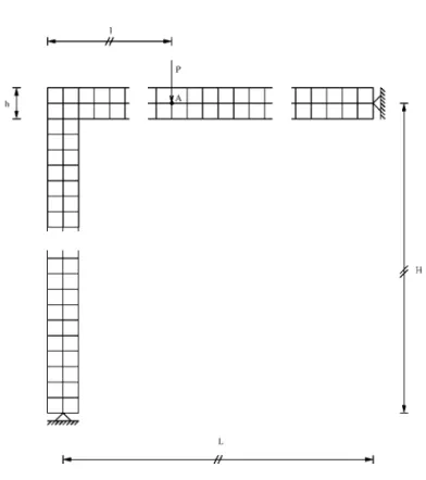
5.5. Lee frame
Figure 9. Lee frame (L= 120 cm, H= 120 cm, l= 24 cm, h= 2 cm, Thickness = 3 cm,E= 720 kN=cm2, v= 0:3,P= 1 kN).
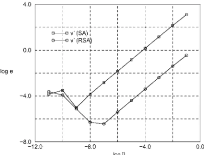
This structure has a highly non-linear behaviour with two limit points and a snap-back behaviour after the rst limit point. However, in the present paper, the displacement v of node A and the respective sensitivity v′ are computed for a load factor (= 1:8) before the rst limit point. The SA sensitivity errors as a function of the relative perturbations are depicted in Figure 10.
The displacement eld of this structure is characterized by large rigid body rotations, there-fore the semi-analytical method generates very inaccurate results, as shown in Figure 10. The improvement provided by the proposed method is very signicant for almost the entire range of relative perturbations. For the range of 10−5 to 10−10, the relative errors of this method
are smaller than 0:1 per cent.
As in previous examples, the relative errors for both methods decrease almost linearly (in the log scale) with the relative perturbation up to the point where the round-o errors become signicant. In this range, the errors of the proposed method are approximately 100 times smaller than the errors of the conventional SA method.
6. CONCLUSIONS
Figure 10. Relative errors for the Lee frame.
analysis is presented. The equilibrium equations relating the element internal force vector and the rigid body modes are the starting point of the present formulation. The dierentiation of these equilibrium equations w.r.t the design variables yields important relations involving the element internal force vector, the rigid body motions, and their derivatives. It is worthwhile pointing out that the rigid body modes and their derivatives depend only on the structural problem at hand, and not on the element formulation.
The main idea of the RSA method is the decomposition of the derivative of the element internal force vector, which appears in the expression of the pseudo-load vector, into a compo-nent in the space spanned by the rigid body modes and another one orthogonal to this space. Using the relations mentioned above, the components in the space of rigid body modes are evaluated in an exact manner, provided that the derivatives of rigid body modes are exactly computed.
This procedure allows the elimination of the abnormal errors presented by the conventional SA method for structures whose displacement eld is dominated by the rigid body rotations of individual elements. The proposed method can be implemented in a generic form since the rigid body modes and their derivatives do not depend on the particular element formulation. The additional terms which appear in the expression of the pseudo-load vector can be evaluated very eciently since they involve only dot products. It is important to note that, due to its generality, the RSA method is particularly suited for implementation using the OOP paradigm. The examples presented in this paper show the improvement of the shape sensitivities computed by the RSA method in comparison with the conventional SA sensitivities, specially when greater rigid body rotations are present. For these structures, the relative error in the design sensitivity can be reduced by a factor of 100.
The performance of the method is more impressive for relative perturbations larger than 10−7, where the truncation errors of the SA method are dominant. For relative perturbations
smaller than 10−7, the round-o errors become dominant, and the dierences between the SA
the numerical examples are related only to geometrically non-linear structures, the proposed method can also be applied to materially non-linear problems.
ACKNOWLEDGEMENTS
The rst author acknowledges the nancial support provided by the CNPq Brazilian Research Agency. The authors would like to thank to TeCGraf (Computer Graphics Technology Group) at PUC-Rio University for providing the computer facilities in which most of the computational work of this paper was performed. The authors acknowledge J.B.M. Sousa Jr. and A.S. de Holanda for their careful reading of the manuscript and valuable suggestions.
REFERENCES
1. Sun Y, Wang S, Gallagher RH. Sensitivity analysis of continuum structures.Computers and Structures1985; 20(5):855–867.
2. El-Sayed MEM, Zumwalt KW. Ecient design sensitivity derivatives for multi-load case as an integrated part of nite element analysis.Computers and Structures 1991;40(6):1461–1467.
3. Parente E Jr., Vaz LE. Shape sensitivity analysis of geometrically nonlinear structures.Design Optimization
1999;1(3):305–327.
4. Barthelemy B, Chon CT, Haftka RT. Accuracy problems associated with semi-analytical derivatives of static response.Finite Element Analysis Design1988;4:249 –265.
5. Cheng G, Olho N. Rigid body motion test against error in semi-analytical sensitivity analysis.Computers and Structures1993;46(3):515–527.
6. Olho N, Rasmussen J, Lund E. A method of ‘exact’ numerical dierentiation for error elimination in nite-element-based semi-analytical shape sensitivity analysis. Mechanics of Structures and Machines 1993; 25(8):1118–1125.
7. Olho N, Lund E. Finite element based engineering design sensitivity analysis and optmization. InAdvances in Structural Optmization, Herskovits J. (ed.). Kluwer Academic Publishers: Dordrecht, 1– 45.
8. Hinton E, Sienz J, Afonso SMB. Experiences with olho’s ‘exact’ semi-analytical algorithm. In WCSMO-1,
First World Congress of Structural and Multidisciplinary Optimization, Olho N, Rozvany GIN. (eds). Goslar, Germany, 1995; 41– 46.
9. de Boer H, van Keulen F. Error analysis of rened semi-analytical design sensitivities.Structural Optimization
1997;14:242–247.
10. van Keulen F, de Boer H. Rigorous improvement of semi-analytical design sensitivities by exact dierentiation of rigid body motions.International Journal for Numerical Methods in Engineering 1998;42:71–91. 11. van Keulen F, de Boer H. Rened semi-analytical design sensitivities for buckling, aiaa-98-4761. In
AIAA=USAF=NASA=ISSMO Symposium on Multidisciplinary Analysis and Optimization, 1998; 420 – 429. 12. de Boer H, van Keulen F. Improved semi-analytic design sensitivities for a linear and nite rotation shell element.
InWCSMO-2,Second World Congress of Structural and Multidisciplinary Optimization, Gutkowski W, Mroz Z. (eds). Zakopane, Poland, 1997; 199 –204.
13. van Keulen F, de Boer H. Accurate design sensitivities for deployable structures by exact dierentiation of rigid body modes.IUTAM-IASS Symposium on Deployable Structures, to appear.
14. de Boer H, van Keulen F. Rened semi-analytical design sensitivities.International Journal of Solid Structures
2000;37:6961–6980.
15. Criseld MA.Non-linear Finite Element Analysis of Solids and Structures, vol. 1, Wiley: New York, 1991. 16. Strang G.Linear Algebra and Its Applications. Saunders: London, (3rd edn).
17. Martha LFCR, Menezes IFM, Lages EN, Parente Jr. E, Pitangueira RLS. An oop class organization for materially nonlinear fe analysis.Proceedings of XVII CILAMCE, Venice, Italy, 1996; 229 –232.
18. Bathe KJ. Finite Element Procedures. Prentice-Hall: Englewood Clis, NJ, 1996.
19. Wriggers P, Simo JC. A general procedure for the direct computation of turning and bifurcation points.
International Journal for Numerical Methods in Engineering1990;30:155–176.
20. Schweizerho KH, Wriggers P. Consistent linearization for path following methods in nonlinear fe analysis.