A note on the population genetic consequences of delayed larval development in insects

A note on the population genetic consequences of delayed larval

development in insects

Marcos Mattoso de Salles and Paulo A. Otto

Departamento de Genética e Biologia Evolutiva, Instituto de Biociências, Universidade de São Paulo,

São Paulo, SP, Brazil.

Abstract

Observations by Dobzhansky’s group in the 1940s suggesting that the presence of recessive genotypes could ac-count for lower larval developmental rates inDrosophila melanogaster were not confirmed at the time and all subse-quent investigations on this subject focused on the analysis of ecological models based on competition among pre-adult individuals. However, a paper published in this journal in 1991 eventually confirmed the finding made by Dobzhansky and his co-workers. In this report, we provide a theoretical analysis of the population genetic effects of a delay in the rate of larval development produced by such a genetic mechanism.

Keywords: difference and differential equations,Drosophila, dynamic systems, larval development, population genetics.

Received: March 11, 2013; Accepted: July 7, 2013.

Introduction

Based on an analysis of samples from natural popula-tions ofDrosophila pseudoobscuracollected from three lo-calities on Mount San Jacinto (California), Dobzhanskyet

al.(1942) showed that homozygotes for genes located on

the second and third chromosomes in this species had a lower developmental rate than expected. These authors suggested that, under controlled culture conditions, the via-bility and developmental rates were dependent on the de-mographic density of the larvae. In contrast to the genetic finding, the latter observation was subsequently confirmed by several authors (Bakker, 1959, 1969; De Witt, 1960;

Robertson, 1963, 1964; Barker and Podger, 1970; Huanget

al., 1971; Tosic and Ayala, 1981; Mather and Caligari,

1981; Ménsua and Moya, 1983; Adellet al., 1988), not only for drosophilid populations but for other insects as well. As a result, all subsequent research on this subject has centered on the analysis of ecological models based on competition among pre-adult individuals. Oliveira and Cordeiro (1981) detected a major gene effect on delayed development in

Drosophila melanogasterthat was later associated with a recessive gene located on the second chromosome of this fly (Oliveiraet al., 1991).

Since the development of molecular genetics in the early 1990s many authors have examined the role of genes involved in the regulation of developmental timing and body size determination inDrosophila. Most of these

stud-ies focused on genes related to apoptosis and to the produc-tion or release of ecdysone and other ecdysteroids (molting hormones). The results of some relevant articles (all deal-ing with this hormone inD. melanogaster) are summarized below. Other authors described the importance of addi-tional gene-controlled systems, such as those involved in the regulation of adenosine deaminase-related growth

fac-tor ADGF-A, in developmental timing (Dolezal et al.,

2005) and in the regulation of the activities of oxidative phosphorylation complexes through nuclear-encoded

mito-chondrial tyrosyl-tRNA synthetases (Meiklejohn et al.,

2013). Oldhamet al.(2000) and Quinnet al.(2012) provide appropriate reviews of this subject.

Sliter and Gilbert (1992) showed that loss of function mutations at thedre4gene caused ecdysteroid deficiency and developmental delay or arrest. Later, Bialeckiet al.

(2002) showed that isoform-specific null mutants for the

orphan memberE75Agene had a reduced ecdysteroid titer

that resulted in developmental delay. McBrayer et al.

(2007) showed that prothoracicotropic (PTTH) hormone production was not essential for molting or metamorphosis but that its lack resulted in significantly delayed larval

de-velopment. Ghoshet al.(2010) showed that the gap gene

giant(gt) regulated ecdysone production through specifica-tion of PTTH and that mutants for this gene exhibited de-layed larval development (in addition to other effects).

The purpose of the present theoretical investigation was to analyze the population genetic effects of a delay in the larval developmental rate produced by an autosomal re-cessive mode of inheritance.

www.sbg.org.br

Send correspondence to Paulo A. Otto. Departamento de Genética e Biologia Evolutiva, Instituto de Biociências, Universidade de São Paulo, Caixa Postal 11461, 05422-970 São Paulo, SP, Brazil. E-mail: otto@usp.br.

Using elements from the theory of finite differences, difference and differential equations, and dynamic systems, we examined the problem based on a model with discrete generations and with the total number of individuals (adults plus larvae) kept constant. We also summarize the results obtained with alternative models involving an increase or decrease in the total population number. The case of contin-uous generations (to be presented in detail elsewhere) is also briefly discussed.

Description of the main model in which the total

number of individuals is kept constant over

discrete generations

The central principle of this model is that the total number of individuals (adults + larvae) is kept constant in a population with discrete generations. For this, letAanda be a pair of segregating alleles at an autosomal locus. In the homozygous state the recessive geneainduces a delay in larval development (increase in the diapause phase), mea-sured in an integer number of generations: crosses therefore take place randomly (panmixia) only among individuals belonging to the same generation. The population size, kept rigorously constant throughout generations, is assumed to be so large that the effects of random sampling genetic drift are negligible. Consequently, the mathematical treatment is deterministic and gene frequencies are interpreted as proba-bilities. The effects of differential migrations, selection pressure and mutation are also considered negligible.

In the equations describing the model we will use the following parameters:N0= number of adults in the initial

population at generation 0; this number equals the total number of individuals (adults plus larvae) at any time or generationK³0;q0= initial frequency of the recessive

al-lelea[q0=f0(a)];p0= initial frequency of the normal allele

A [p0= f0(A) = 1-q0];T= delay in larval development

de-termined by the genotypeaa, measured in an integer num-ber of generations;K= index corresponding to an integer number of generations;NK= number of adult individuals in

the population at theK-th generation;N’K= number of

lar-vae in the population at theK-th generation;qK= frequency

of the recessive geneaamong adults at theK-th generation; pK= frequency of the normal allele, also among adults

be-longing to theK-th generation;QK= frequency of the

re-cessive gene in the total population (adults plus larvae) at theK-th generation;PK= frequency of the normal allele,

also in the total population, at theK-th generation (PK= 1

-QK).

Derivation of pertinent equations

Based on the foregoing definitions:

(a) the total number of adults at generationKis given by

NK= NK-1(1-qK-12)ifK£Tor

NK= NK-1(1-qK-12) + NK-1-TqK-1-T2ifK > T;

(b) the genotypic proportions amongAA,Aaandaa

adult individuals at generationKare, respectively:

(NK-1/NK)pK-12, (NK-1/NK)2pK-1qK-1, and0ifK£T

or

(NK-1/NK)pK-12, (NK-1/NK)2pK-1qK-1, and

(NK-1-T/NK)qK-1-T2ifK > T;

(c) the number of larvaeaapresent at generationK after the maturation of normal individuals is given by

N’K= N0q02+ N1q12+ ... + NK-1qK-12ifK£Tor

N’K= NK-TqK-T2+ NK-T+1qK-T+12+...+ NK-1qK-12if

K > T.

Using the foregoing equations, it is not difficult to show thatNK+1+N’K+1= NK+ N’K= ... = N0+ 0 = N0and

that, if PK = f(A) in the total population, then PK =

(NK/N0)pK= (NK/N0)(N0p0/NK) = p0,i.e., allele frequencies

and the number of individuals remain constant when the whole population (adults plus larvae) is considered, as as-sumed by the model.

ForK£_{T, we have, among adults of the population, a}

mechanism similar to the classic model of total selection

against homozygous recessive individualsaa, despite the

absence of selection against any individual of the popula-tion (when adults and larvae are considered together), as shown by the equations derived in the previous paragraph. This results inqK+1= qK/(1+qK), a recurrence equation that

has the general solution in simple analytical form qK =

q0/(1+Kq0).

ForK > T, we have

NK+1= NK(1-qK2) + NK-TqK-T2=

NK(1-qK)(1+qK) + NK-TqK-T2=

NKpK(2-pK) + NK-T(1-pK-T)2.

Since pK+1 = (NKpK2+NKpKqK)/NK+1 = NKpK/NK+1

and, hence, NK = N0p0/pK, it follows that N0p0/pK+1 =

N0p0(2-pK) + N0p0(1-pK-T)2/pK-Tand

1/pK+1= 1/pK-T+ pK-T- pK,

pK+ 1/pK+1= pK-T+ 1/pK-T,

or, sincepK= N0p0/NK, we also obtain

NK+1= NK-T+ (N0p0)2(1/NK-T- 1/NK).

Dynamic behavior of allele frequencies

Below, we analyze the behavior of allele frequencies pKandqK.

ForK£_{T,pK= (p0+ Kq0)/(1 + Kq0),i.e.,pKis a}

Analysis of the functionf(x) = x + 1/xin the interval0 < x < 1shows thatf’(x) = 1 - 1/x2< 0;f(x)is therefore a monotonically decreasing function ofxin this interval.

IfpK> pK-T, then we havepK+ 1/pK< pK-T+ 1/pK-T=

pK+ 1/pK+1and, therefore,pK+1< pK; similarly,pK< pK-T

implies thatpK+1> pK, andpK= pK-Timplies thatpK+1= pK.

In the interval0 < K£_{T,pKincreases such that when}

KsurpassesT, we havepK> pK-T;pKthen decreases to a

new point wherepK< pK-Tis reached and we will then have

another increase inpK, and so on. Thus, there will be an

os-cillation in gene frequencies among adults of the

popula-tion. With the passing of generations, i.e., when K

in-creases, the variations become smaller. In the limit case,

when K tends to infinity, the gene frequencies reach an

equilibrium (pinf= pe, qinf= qe).

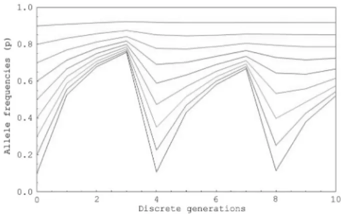
Figures 1-3 show numerical examples of oscillatory convergence to equilibrium points (pe) over 10 generations

of random crosses, for populations starting with initial gene frequenciesp0=0.1, ... ,0.9andTvalues ofT = 1,2, and3.

These graphs and others shown in this paper were prepared

using routines and packages from Mathematicaâ v.8.0

(Wolfram Research).

The preliminary global analysis presented above al-ready shows a point of real theoretical interest, namely, that despite intense selective pressure among adult individuals (but not among the total population of adults plus larvae), the recessive allele is never eliminated from the population, but rather is kept in equilibrium at a pointqe> 0. This is true

except when the number of generations involved in the de-velopmental delay is very large or tends to infinity such that alleleais practically eliminated from the adult population and all larvae fail to develop.

Equilibrium gene frequencies

In a generic instant we have the following population composition (Figure 4).

If we consider an equilibrium situation where

NK+1= NK= NK-1= NK-2= ... = NK-T= Ne

qK+1= qK= qK-1= qK-2= ... = qK-T= qe= 1-pe,

fromNK+ N’K= N0it follows thatNe+ TNeqe2= N0.

Since Ne = N0p0/pe, it follows that

N0p0(1+Tqe2)/(1-qe) = N0, and, hence,p0+ Tp0qe2= 1-qe

and, finally,

qe= [(1+4Tp0q0)1/2-1]/(2Tp0) =

2q0/[(1+4Tp0q0)1/2+1].

Figure 1- Oscillatory convergence of allele frequencies (ordinate axis) to equilibrium points for populations starting with initial allele frequencies ofp0= 0.1, ..., 0.9 andT = 1generation of delayed larval development over a period of 10 discrete generations (abscissa axis).

Figure 2- Oscillatory convergence of allele frequencies (ordinate axis) to equilibrium points for populations starting with initial allele frequencies ofp0= 0.1, ..., 0.9 andT = 2generations of delayed larval development over a period of 10 discrete generations (abscissa axis).

Figure 3- Oscillatory convergence of allele frequencies (ordinate axis) to equilibrium points for populations starting with initial frequencies of

p0=0.1, ...,0.9andT = 3generations of delayed larval development over a period of 10 discrete generations (abscissa axis).

As expected,qe= q0ifT = 0(simple case of panmixia

without selection) andqe= 0ifT =¥(special case of

com-plete selection against recessive individualsaa). Considering that:

pK= NK-1pK-1/NK= N0p0/NKfor anyK,

NK= NK-1(1-qK-12)for anyK£T,

and

NK= NK-1(1-qK-12) + NK-T-1qK-T-12for anyK > T,

it is not difficult to show that the recurrence equation1/pK+1

= pK-T+ 1/pK-T- pKcan be rewritten in the more convenient

form

1/pK= 1/p0-S[j = 1, T]{(1-pK-j)2/pK-j}.

This recurrence equation allows straightforward deri-vation of the equilibrium pointpe. Indeed, whenKtends to

infinity, the limit for the right-hand side of the above equa-tion is1/p0- T(1-pe)2/peand it follows thatpe= p0(1+Tqe2)

andpe= 1 - qe= 1 - [(1+4Tp0q0)1/2-1]/(2Tp0).

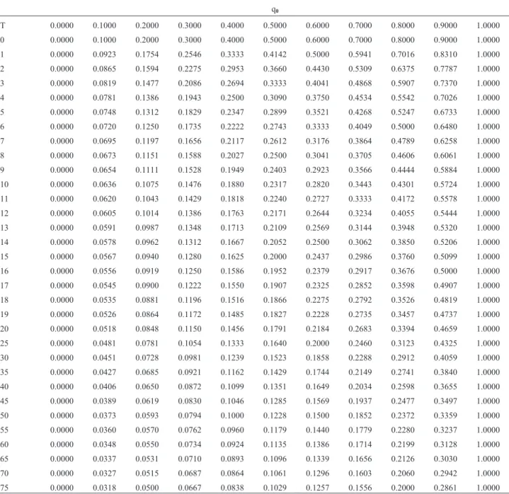
Table 1 shows the sets of equilibrium pointsqe for

several values ofT, as a function of the initial valuesq0=

0.0,0.1, ...,0.9,1.0.

Figure 5 shows the sets of equilibrium valuesqeas a

function of the initial frequency valuesq0andT varying

from 0 to 15.

Table 1- Equilibrium points (qe) as a function ofTand of the initial allele frequency (q0).

q0

T 0.0000 0.1000 0.2000 0.3000 0.4000 0.5000 0.6000 0.7000 0.8000 0.9000 1.0000

0 0.0000 0.1000 0.2000 0.3000 0.4000 0.5000 0.6000 0.7000 0.8000 0.9000 1.0000

1 0.0000 0.0923 0.1754 0.2546 0.3333 0.4142 0.5000 0.5941 0.7016 0.8310 1.0000

2 0.0000 0.0865 0.1594 0.2275 0.2953 0.3660 0.4430 0.5309 0.6375 0.7787 1.0000

3 0.0000 0.0819 0.1477 0.2086 0.2694 0.3333 0.4041 0.4868 0.5907 0.7370 1.0000

4 0.0000 0.0781 0.1386 0.1943 0.2500 0.3090 0.3750 0.4534 0.5542 0.7026 1.0000

5 0.0000 0.0748 0.1312 0.1829 0.2347 0.2899 0.3521 0.4268 0.5247 0.6733 1.0000

6 0.0000 0.0720 0.1250 0.1735 0.2222 0.2743 0.3333 0.4049 0.5000 0.6480 1.0000

7 0.0000 0.0695 0.1197 0.1656 0.2117 0.2612 0.3176 0.3864 0.4789 0.6258 1.0000

8 0.0000 0.0673 0.1151 0.1588 0.2027 0.2500 0.3041 0.3705 0.4606 0.6061 1.0000

9 0.0000 0.0654 0.1111 0.1528 0.1949 0.2403 0.2923 0.3566 0.4444 0.5884 1.0000

10 0.0000 0.0636 0.1075 0.1476 0.1880 0.2317 0.2820 0.3443 0.4301 0.5724 1.0000

11 0.0000 0.0620 0.1043 0.1429 0.1818 0.2240 0.2727 0.3333 0.4172 0.5578 1.0000

12 0.0000 0.0605 0.1014 0.1386 0.1763 0.2171 0.2644 0.3234 0.4055 0.5444 1.0000

13 0.0000 0.0591 0.0987 0.1348 0.1713 0.2109 0.2569 0.3144 0.3948 0.5320 1.0000

14 0.0000 0.0578 0.0962 0.1312 0.1667 0.2052 0.2500 0.3062 0.3850 0.5206 1.0000

15 0.0000 0.0567 0.0940 0.1280 0.1625 0.2000 0.2437 0.2986 0.3760 0.5099 1.0000

16 0.0000 0.0556 0.0919 0.1250 0.1586 0.1952 0.2379 0.2917 0.3676 0.5000 1.0000

17 0.0000 0.0545 0.0900 0.1222 0.1550 0.1907 0.2325 0.2852 0.3598 0.4907 1.0000

18 0.0000 0.0535 0.0881 0.1196 0.1516 0.1866 0.2275 0.2792 0.3526 0.4819 1.0000

19 0.0000 0.0526 0.0864 0.1172 0.1485 0.1827 0.2228 0.2735 0.3457 0.4737 1.0000

20 0.0000 0.0518 0.0848 0.1150 0.1456 0.1791 0.2184 0.2683 0.3394 0.4659 1.0000

25 0.0000 0.0481 0.0781 0.1054 0.1333 0.1640 0.2000 0.2460 0.3123 0.4325 1.0000

30 0.0000 0.0451 0.0728 0.0981 0.1239 0.1523 0.1858 0.2288 0.2912 0.4059 1.0000

35 0.0000 0.0427 0.0685 0.0921 0.1162 0.1429 0.1744 0.2149 0.2741 0.3840 1.0000

40 0.0000 0.0406 0.0650 0.0872 0.1099 0.1351 0.1649 0.2034 0.2598 0.3655 1.0000

45 0.0000 0.0389 0.0619 0.0830 0.1046 0.1285 0.1569 0.1937 0.2477 0.3497 1.0000

50 0.0000 0.0373 0.0593 0.0794 0.1000 0.1228 0.1500 0.1852 0.2372 0.3359 1.0000

55 0.0000 0.0360 0.0570 0.0762 0.0960 0.1179 0.1440 0.1779 0.2280 0.3237 1.0000

60 0.0000 0.0348 0.0550 0.0734 0.0924 0.1135 0.1386 0.1714 0.2199 0.3128 1.0000

65 0.0000 0.0337 0.0531 0.0710 0.0893 0.1096 0.1339 0.1656 0.2126 0.3030 1.0000

70 0.0000 0.0327 0.0515 0.0687 0.0864 0.1061 0.1296 0.1603 0.2060 0.2942 1.0000

For the caseT = 1, the recurrence equation above can be rewritten as

1/pK+1= 1/p0- (1-pK)2/pKor pK+1=

p0pK/[pK-p0(1-pK)2].

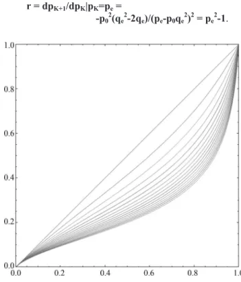
The eigenvaluerresponsible for the convergence of the series{p0, ...,pe} is obtained by directly differentiating

pK+1= f(pK)at equilibrium pointpe:

r = dpK+1/dpK|pK=pe=

-p02(qe2-2qe)/(pe-p0qe2)2= pe2-1.

Since|r| = |pe2-1| < 1for any value ofpein the interval

0 < pe< 1, the equilibrium pointpeis asymptotically stable

and convergence to this point occurs at a geometric rate. Sinceris always smaller than zero in this interval, conver-gence to equilibrium is oscillatory.

Figure 6 shows the values ofrandqeas functions of

the initial gene frequencyq0for the caseT = 1.

For a generic value ofTthe method that follows is used for determining convergence rates as well as equilib-rium properties.

q0

80 0.0000 0.0310 0.0486 0.0648 0.0815 0.1000 0.1222 0.1512 0.1945 0.2787 1.0000

85 0.0000 0.0302 0.0474 0.0631 0.0793 0.0973 0.1189 0.1472 0.1895 0.2718 1.0000

90 0.0000 0.0295 0.0462 0.0615 0.0773 0.0949 0.1160 0.1436 0.1849 0.2655 1.0000

95 0.0000 0.0288 0.0451 0.0601 0.0755 0.0926 0.1132 0.1402 0.1806 0.2596 1.0000

100 0.0000 0.0282 0.0441 0.0587 0.0737 0.0905 0.1106 0.1370 0.1766 0.2541 1.0000

105 0.0000 0.0277 0.0432 0.0574 0.0721 0.0885 0.1082 0.1340 0.1728 0.2490 1.0000

110 0.0000 0.0271 0.0423 0.0563 0.0706 0.0867 0.1060 0.1313 0.1693 0.2442 1.0000

115 0.0000 0.0266 0.0415 0.0552 0.0692 0.0850 0.1039 0.1287 0.1660 0.2396 1.0000

120 0.0000 0.0261 0.0407 0.0541 0.0679 0.0833 0.1019 0.1262 0.1629 0.2353 1.0000

125 0.0000 0.0257 0.0400 0.0531 0.0667 0.0818 0.1000 0.1239 0.1600 0.2313 1.0000

130 0.0000 0.0253 0.0393 0.0522 0.0655 0.0804 0.0982 0.1218 0.1572 0.2275 1.0000

135 0.0000 0.0249 0.0387 0.0513 0.0644 0.0790 0.0966 0.1197 0.1546 0.2238 1.0000

140 0.0000 0.0245 0.0380 0.0505 0.0633 0.0777 0.0950 0.1177 0.1521 0.2203 1.0000

145 0.0000 0.0241 0.0374 0.0497 0.0623 0.0764 0.0935 0.1159 0.1497 0.2170 1.0000

150 0.0000 0.0238 0.0369 0.0489 0.0613 0.0753 0.0920 0.1141 0.1475 0.2139 1.0000

inf 0.0000 0.0000 0.0000 0.0000 0.0000 0.0000 0.0000 0.0000 0.0000 0.0000 0.0000

Table 1 (cont.)

Figure 5- Sets of stable equilibrium valuesqe(ordinate axis) as a function of initialq0values (abscissa aixs) forTvalues varying from 0 to 15.

Equilibrium dynamics

As shown above, for anyK > T,

1/pK= 1/p0-S[j = 1,T]{(1-pK-j)2/pK-j}or

pK= 1/[1/p0-S[j = 1,T]{(1-pK-j)2/pK-j}].

We then define a set ofTvariables as follows: x1(K) pK

x2(K) pK-1

. .

XK= ( . ) = ( . ).

. .

. .

xT(K) pK-T+1

Since

pK+1= [1/p0-S[j = 1,T]{(1-pK-j+1)2/pK-j+1}] - 1

we have:

x1(K+1) = f[x1(K), x2(K), x3(K+1), x4(K), ... , xT(K)]

x2(K+1) = x1(K)

x3(K+1) = x2(K)

x4(K+1) = x3(K)

...

xT(K+1) = xT-1(K).

Considering the equilibrium point, at which x1(K) pe

x2(K) pe

. .

Xe= ( . ) = ( . ),

. .

. .

xT(K) pe

we have, in an infinitesimal neighborhood of this point, DX(K+1) = A.DX(K), or, in expanded form,

Dx1 a a a ... a a Dx1

Dx2 1 0 0 ... 0 0 Dx2

Dx3 0 1 0 ... 0 0 Dx3

(.)K+1= (...) (.)K

. ... . . ... .

DxT 0 0 0 ... 1 0 DxT

where

a = df/dx1(K) |x=xe= df/dx2(K) |x=xe= ... =

= df/dxj(K) |x=xe=

= pe2- 1.

The eigenvaluesr1,r2, ... ,rTare the solutions of the

characteristic equation

det(A-rI) = (-1)T(1+r+r2+ … +rT-1- rT/a) = 0

or

rT/a = 1 + r + r2+ r3+ ... + rT-2+ rT-1,

which can also be rewritten asrT/a = (1-rT)/(1-r), r¹_1.

Based on the functionf(r) = rT+1- (a+1)rT+ a, r¹_1,

-1 < a < 0, it can be shown thatf(0) = a < 0,f(1) = 0and df(r)/dr = f’(r) = (T+1)rT- T(a+1)rT-1. Also, asrtends to +¥_{,f(r)tends to+infand asrtends to-}¥_{,f(r)tends to+}¥_if

Tis odd, and to-¥_{ifTis even. When T is even,f’(r)is an}

increasing function ofrin the open interval (-¥_{, 0),}

de-creasing in the open interval(0, (a+1)T/(T+1))and again increasing forr > 0. Therefore,r = 0is a relative maximum andr = (a+1)T/(T+1)a relative minimum. WhenTis odd, f’(r)is a decreasing function ofrin the open interval(-inf, (a+1)T/(T+1)) and an increasing function of r for r > (a+1)T/(T+1). Therefore,r = 0in the case whenTis odd is an inflection point, whereasr = (a+1)T/(T+1)is a relative

minimum (as in the case whenTis even). Hence, we

con-clude that whenTis even, the equationrT+1- (a+1)rT+ a =

0, r¹_{1, -1 < a < 0does not have any real root sincef(r)}

tends to-¥_{asrtends to-}¥_{; whenTis odd, the above}

equa-tion has just one real negative root sincef(r)tends to+¥_as

rtends to-¥_.

For the casesT = 1to4it is possible to obtain explicit solutions in simple analytical form for the values of the eigenvaluesr; forT > 4the eigenvalues can be determined using numerical methods. Analytical procedures applied in the caseT < 5and extensive numerical analysis of the equa-tion for any values ofT > 4have shown that (a) whenTis odd, there is always one real eigenvalue, with|ri| < 1and -1 < ri < 0, and(T-1)/2pairs of complex conjugatesrj,k=A

±_{iB, with(A}2_+B2₎1/2_{< 1for any initial gene frequencyp0;}

(b) whenTis even, there are always onlyT/2pairs of com-plex conjugates with the same properties as stated before. We therefore conclude that the set of equilibrium points pe= f(p0, T)is a stable one, with convergence always

oc-curring to it for any initial valuep0in the open interval

(0, 1)and for any integer value ofT.

Description of the model in which there are

fluctuations in the total number of individuals

In order to study the effect of an increase or decrease in population size, it is enough to introduce the additional parameterc:N1p1= cN0p0into equationN1p1= N0p0of the

previous section. Consideration of this parameter leads straightforwardly the equation pK+1 = 1/[2-pK+(1-pK-T)2/

(cTpK-T)],K > T. This is the same equation obtained in the

analysis of the constant population size model ifc = 1. At equilibrium,pK+1= pK= pK-T= peand the above

equation reduces tope(1-pe)2(1-cT) = 0, c¹1. Whenc¹1,

the only possible solutions for the foregoing equation are pe=0andpe= 1,i.e., the normal allele is completely lost or

fixed. Intuitively, it is easy to show thatpe= 0whenc < 1

in-verse,i.e., whenc > 1(population increasing in size), is also obviously true since proportionally fewer recessive genes will be introduced into the adult population by emerging larvae. Clearly, then,petends to1as generations go by.

Brief remarks on a model with continuous

generations

LetP(t),R(t),Q(t)andL(t)be the normalized pro-portions {P(t) + R(t) + Q(t) + L(t) = 1} of adultsAA,Aa andaa, and larvaeaa in generationt. Among adults, the normalized genotypic proportions are given by:

f(AA) = P’ = P/(1-L)

f(Aa) = R’ = R/(1-L)

f(aa) = Q’ = Q/(1-L)

and the corresponding allelic frequenciesf(A) andf(a)by

f(A) = p(t) = P’ + R’/2

f(a) = q(t) = Q’ + R’/2.

In the total population (adults + larvae), the allelic fre-quencies are given by

p(t) = P + R/2

and

q(t) = Q + L + R/2, p(t) + q(t) = 1.

After a time interval Dt, the frequency of allele A among adults of the population is given by

p(t+Dt) = [N(t).p2(t) + N(t).2p(t)q(t)/2]/N(t+Dt) =

= {N(t).p(t)[p(t)+q(t)]}/N(t+Dt) =

= N(t).p(t)/N(t+Dt),

with the restrictionN(t+Dt).p(t+Dt) = N(t).p(t) = N0p0=

constant, as in the discrete model.

The expression forp(t+Dt)can be used for quantita-tive analysis (to be presented elsewhere) in the case of con-tinuous generations. One expects that equilibrium values for any fraction0 <e_{< 1inT < T+}e_{< T+1would}

interpo-late between the equilibrium curves that represent the set of equilibrium points for the integer cases ofTandT+1 gener-ations in delayed larval development.

Acknowledgments

The subject of this paper was suggested to Paulo A. Otto in the 1980s by the late Prof. Luiz Edmundo de Magalhães, at the time a professor in the Department of Bi-ology at USP. Subsequently, a congress note on this subject (Ottoet al., 1990) was published with the co-authorship of Prof. Magalhães and a PhD student, Luiz Antonio Bene-detti, now a professor in the Mathematics Department of

the Federal University of Uberlândia in Minas Gerais. This work was partly funded by FAPESP.

References

Adell JC, Moya A and Botella LM (1988) Larval arrest in the de-velopment of the lygaeid bugSpilostethus pandurus. Evol Biol 2:251-260.

Bakker K (1959) Feeding period, growth and pupation in larvae of Drosophila melanogaster. Entomol Exp Appl 2:171-186. Bakker K (1969) Selection for rate of growth and its influence on

competitive ability of larvae ofDrosophila melanogaster. Netherl J Zool 19:541-595.

Barker JSF and Podger RN (1970) Interspecific competition be-tweenDrosophila melanogasterandDrosophila simulans: Effects of larval density on viability, developmental period and adult body size. Ecology 51:170-189.

Bialecki M, Shilton A, Fichtenberg C, Seagraves WA and Thum-mel CS (2002) Loss of the ecdysteroid-inducible E75A or-phan nuclear receptor uncouples molting from metamorpho-sis inDrosophila. Dev Cell 3:209-220.

De Witt CT (1960) On competition. Versl Landbouwk Onderz 66:8-82.

Dobzhansky T, Holz AM and Spassky B (1942) Genetics of natu-ral populations. VIII. Concealed variability in the second and the fourth chromosomes ofDrosophila pseudoobscura and its bearing on the problem of heterosis. Genetics 27:463-490.

Dolezal T, Dolezelova E, Zurovec M and Bryant PJ (2005) A role for adenosine deaminase inDrosophilalarval development. PloS Biol 3:e201.

Ghosh A, McBrayer Z and O’Connor MB (2010) TheDrosophila gap gene giant regulates ecdysone production through speci-fication of the PTTH-producing neurons. Dev Biol 347:271-278.

Huang SL, Singh M and Kojima KI (1971) A study of fre-quency-dependent selection observed in the esterase-6 locus of Drosophila melanogaster using a conditioned media method. Genetics 68:97-104.

Mather K and Caligari PDS (1981) Competitive interactions in Drosophila melanogaster. II. Measurement of competition. Heredity 46:239-244.

McBrayer Z, Ono H, Shimell MJ, Parvy JP, Beckstead RB, War-ren JT, Thummel CS, Dauphin-Villemant C, Gilbert LI and O’Connor MB (2007) Prothoracicotrophic hormone regu-lates developmental timing and body size in Drosophila. Dev Cell 13:857-871.

Meiklejohn CD, Holmbeck MA, Siddiq MA, Abt DN, Rand DM and Montooth KL (2013) An incompatibility between a mi-tochondrial tRNA and its nuclear-encoded tRNA synthetase compromises development and fitness inDrosophila. PloS Genet 9:e1003238.

Ménsua JL and Moya A (1983) Stopped development in over-crowded cultures of Drosophila melanogaster. Heredity 51:347-352.

Oldham S, Böhni R, Stocker H, Brogiolo W and Hafen E (2000) Genetic control of size inDrosophila. Proc R Soc Lond B 355:945-952.

Oliveira AK, Monjelo LAS and Cordeiro AR (1991) A second chromosome major gene for developmental rate in Drosophila melanogaster. Rev Bras Genet 14:953-965.

Otto PA, Benedetti LA and Magalhães LE (1990) Efeitos do atraso de desenvolvimento larval sobre as frequências aléli-cas em uma população. Resumos do XXXVI Congresso Nacional de Genética, Caxambu, pp 167-167.

Quinn L, Lin J, Cranna N, Lee JEA, Mitchell N and Hannan R (2012) Steroid hormones inDrosophila: How ecdysone co-ordinates developmental signalling with cell growth and di-vision. In: Abduljabbar H (ed) Steroid – Basic Science. Intech, Rijeka, pp 141-168.

Robertson FV (1963) The ecological genetics of growth in Drosophila. 6. The genetic correlation between the duration

of the larval period and body size in relation to larval diet. Genet Res 4:74-92.

Robertson FV (1964) The ecological genetics of growth in Drosophila. 7. The role of canalization in the stability of growth relations. Genet Res 5:107-126.

Sliter TJ and Gilbert LI (1992) Developmental arrest and ecdys-teroid deficiency resulting from mutations at the dre4 locus ofDrosophila. Genetics 130:555-568.

Tosic M and Ayala FJ (1981) Density- and frequency-dependent selection at the Mdh-2 locus inDrosophila pseudoobscura. Genetics 97:679-701.

Associate Editor: Louis Bernard Klaczko