ABSTRACT: This study aimed to map the stem biomass of an even-aged eucalyptus plantation in southeastern Brazil based on canopy height profile (CHPs) statistics using wall-to-wall discrete return airborne laser scanning (ALS), and compare the results with alternative maps generated by ordinary kriging interpolation from field-derived measurements. The assessment of stem bio-mass with ALS data was carried out using regression analysis methods. Initially, CHPs were determined to express the distribution of laser point heights in the ALS cloud for each sample plot. The probability density function (pdf) used was the Weibull distribution, with two parameters that in a secondary task, were used as explanatory variables to model stem biomass. ALS metrics such as height percentiles, dispersion of heights, and proportion of points were also investigated. A simple linear regression model of stem biomass as a function of the Weibull scale parameter showed high correlation (adj.R² = 0.89). The alternative model considering the 30th percentile and the Weibull shape parameter slightly improved the quality of the estimation (adj. R² = 0.93). Stem biomass maps based on the Weibull scale parameter doubled the accuracy of the ordinary kriging approach (relative root mean square error = 6 % and 13 %, respectively). Keywords: LiDAR, basal area, biometric model, forest inventory, fast-growing plantations
represented by a probability function is a convenient way of summarizing and retrieving the canopy vertical form (Coops et al., 2007). The Weibull probability densi-ty function (pdf) has been used to model vertical profiles thanks to its flexibility in characterizing different types of vegetation, and its parameters of scale and shape were successfully correlated with above ground attributes, such as height of trees, density of stems, and diameter at breast height (Coops et al., 2007; Mori and Hagihara, 1991). In Brazil, ALS technology has been used for ter-rain modeling, but applications involving assessment and mapping of biomass in eucalypt stands are still in-cipient (Packalén et al., 2011; Silva et al., 2014; Vauh-konen et al., 2011). This study aimed to map the stem biomass stock based on canopy height profiles statistics using ALS data of an even-aged eucalypt plantation, in southeastern Brazil, and compare the results with alter-native maps generated by ordinary kriging interpolation from field-derived measurements.
Materials and Methods
Study site
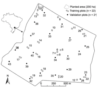
The study site is located in the state of São Paulo, southeastern Brazil (22º58’04” S; 48º43’40” W) (Figure 1). The area is approximately 200 ha and is composed of a 6.5-year-old Eucalyptus grandis (W. Hill ex Maiden) plantation with seedlings coming from a fourth-genera-tion seed orchard (Campoe et al., 2012). The stands were planted in December 2002, with an approximate density of 1600 trees ha−1 (3.75 m × 1.6 m) following minimum site preparation (Gonçalves et al., 2013). The Köppen cli-mate type is Cfa; with mean annual temperature equal 1University of São Paulo/ESALQ – Dept. of Forest Science,
Av. Pádua Dias, 11 − 13418-900 − Piracicaba, SP − Brazil. 2Forestry Science and Research Institute, Av. Comendador Pedro Morgante, 3500 − 13415-000 − Piracicaba, SP − Brazil.
3North Carolina State University – Dept. of Forestry and Environmental Resources, Jordan Hall, 3108 − 27695-8008 − Raleigh, NC – United States of America.
*Corresponding author <[email protected]>
Edited by: Rafael Rubilar Pons
Assessing biomass based on canopy height profiles using airborne laser scanning
André Gracioso Peres Silva1, Eric Bastos Görgens1, Otávio Camargo Campoe2, Clayton Alcarde Alvares2,3, José Luiz Stape3, Luiz Carlos Estraviz Rodriguez1*
Received February 13, 2015
Accepted July 06, 2015
data in eucalypt plantations
Introduction
Current methods of forest inventory are based on the direct surveying of trees and sampling of ground plots (Campos and Leite, 2013). Statistical models gen-erated to predict average estimates of stand attributes and their spatial variability are assessed only sporadi-cally (Zhou et al., 2013). Data interpolation techniques can be used to assess stand spatial structure, yet they are limited by the sampling intensity of ground plots, which is usually insufficient to yield precise estimates (Bouvier et al., 2015; Viana et al., 2012). On the other hand, in-tegrating remotely sensed data is an actual possibility, as it can be acquired to a great extent, within a short time and at reasonable prices (Hummel et al., 2011). Airborne laser scanning (ALS) technology is a potential remote sensing tool, as it can provide data on multiple strata of the canopy, while passive sensors cannot (Mag-nussen and Boudewyn, 1998; Næsset, 1997). The laser sensor records tridimensional coordinates over the sur-veyed area by collecting the time in which a laser pulse takes to go back to the aircraft after being reflected by the target. The result is a georeferenced 3D point cloud with high spatial resolution (Baltsavias, 1999; Reutebuch et al., 2005).
to 19.4 ºC and mean annual precipitation totaling 1300 mm (Alvares et al., 2013). The site relief is mainly flat to soft wavy, and the altitude approximately 750 m (Cam-poe et al., 2012).
Field measurements and plot summaries
Figure 1 shows the network of inventory ground plots in the study site. They were divided into 22 training plots and 21 validation plots. Plots 1 to 12 (457 m2 to 574 m2) were established for research related to ecophysiol-ogy. Their location covered the site’s productivity range after a census of diameter at breast height was carried out (Campoe et al., 2012). In addition, plots 13 to 22 (811 m2 to 881 m2) were designed specifically for ALS investiga-tions. Plots 23 to 43 (240 m2) are permanent ground plots of continuous inventory owned by the forest producer.
Field measurements were conducted in the train-ing plots in July 2009, and July 2008, in the validation plots (Table 1). Diameter at breast height (DBH, 1.3 m above ground level) and total tree height were measured on all plots. Stem dry biomass was estimated using the following local-specific allometric equation derived from destructive sampling in Sep 2008 (Campoe et al., 2012) (Eq. 1).
ˆ . .
Bi= −0 58 147 1+ D Hi i
2 (1)
where: Bˆi= dry stem biomass per tree (kg per tree), Di = diameter at breast height (cm), Hi = total height (m).
Airborne laser scanning (ALS) data
The ALS survey was undertaken during Apr 2009, a period of the year with maximum stable leaf area index (LAI) (le Maire et al., 2011). The flight mission was con-ducted by a twin-engined light aircraft equipped with a discrete-return small footprint laser scanner (laser
wavelength = 1064 nm). The parameters from the flight mission and the scanning process were as follows: flight height = 900 m; flight speed = 132 km h−1; swath width = 235 m; swath overlap = 30 %; scanning angle = 15º; scanning frequency = 74 Hz; frequency of pulse emis-sion = 110 kHz; footprint = 21 cm; point density = 6.5 pts m−2; standard deviation of point density = 2 pts m−2.
GPS observations from ground and aircraft were processed in a method to obtain a unique and adjusted cinematic solution to a well-known coordinate system, using the Waypoint GraphNav software. A digital ele-vation model (DEM) was generated with a one meter resolution, after ground points were labeled with the Multiscale Curvature Classification algorithm (MCC-LiDAR) (Evans and Hudak, 2007). The DEM was sub-tracted from all point elevations to remove topographic variations (normalization process). Then, the normalized point cloud was clipped to the same locations as the in-ventory field plots. The Fusion LiDAR Toolkit software was used to normalize the point cloud (clipdata), to clip plots using shapefiles (polyclipdata) and to extract ALS metrics (cloudmetrics).
We tried to select metrics based on a priori knowl-edge in an attempt to improve the capacity of the model generalization (Bouvier et al., 2015). Among the met-rics extracted from each ALS plot, we focused on using height percentiles. A percentile x is the height z in which x % of points in the ALS cloud are beneath z. We tested the percentiles which predicted better basal area and volume in Zonete et al. (2010): first return percentiles 10, 30, 70, 90. Moreover, we selected metrics such as mean height, standard deviation and variance of heights, all of them also being derived from first returns. These metrics were calculated disregarding laser points with a height less than 2 m (Næsset, 2002; Zonete et al., 2010). We also parameterized a metric of density, which we named p_understory consisting of the proportion of laser points between 0.3 and 15 meters in height and the laser points between ground, (0 meters) and 15-meters in height. The 15-meter threshold was set based on visual inspection of the point cloud and on field experience. In this case, all return echoes were used to increase the sample of points in the understory layer.
Figure 1 – Location map of the study site (22º58’04” S; 48º43’40” W; southeastern Brazil).
Table 1 – Summary of field measurements in the eucalypt plantation site.
Training plots (n = 22) Validation plots (n = 21) Stat. Surv. DBH G H B Stat. Surv. DBH G H B
- % cm m² ha−1 m Mg ha−1 - % cm m² ha−1 m Mg ha−1
Apparent canopy height profiles (CHPs)
From a set of possible theoretical distributions, we chose the Weibull pdf due to its flexibility in characterizing foliage distributions of different types of vegetation and its potential for fitting skewed data, which is a common fea-ture of forest-derived ALS data (Coops et al., 2007; Dean et al., 2009; Lovell et al., 2003; Magnussen et al., 1999).
The apparent canopy height profiles (CHPs) were obtained by curve-fitting all ALS returns with a height greater than 5 m. The threshold aimed to exclude laser points on the ground, in shrubs, and dominated trees, to eliminate the bimodal effect on the vertical profile (Coops et al., 2007; Lovell et al., 2003). Curve-fitting analysis was carried out applying the maximum likeli-hood estimation technique (Cohen, 1965) using fitdistr in R (R Foundation for Statistical Computing; MASS pack-age). The Weibull pdf with two parameters (scale and shape) is shown in Eq. (2).
f x/ ,α β αβxβ exp αx , x ;α ;β
β
(
)
= − − < < ∞ > >
1 0 0 0 (2)
where: f (x / α,β) = probability density of x; α = scale parameter; β = shape parameter.
A Weibull pdf with a shape parameter equal to 1 reduces to an exponential distribution, while shape val-ues between 3 and 4 will approximate a normal curve. The scale parameter is at the 63.2nd percentile of the distribution (McCool, 2012). The Weibull scale and shape parameters were obtained from the CHPs at each training plot, and they were used as candidate predictors for stem biomass modeling.
Regression modeling of stem biomass with ALS data
The linear relationships between the ALS predic-tors and stem biomass were explored by carrying out a paired sample correlation t-test. We suspended ALS metrics from further analysis when the Pearson’s cor-relation coefficient (ρ) was not significant at 99 % confi-dence level. Regression models were fit by the ordinary least squares method, and the ALS predictors were se-lected using the best subset approach (Lumley, 2009). We used the variance inflation factor (VIF) to detect mul-ticollinearity of explanatory variables (Fox and Monette, 1992). Models with VIF greater than 5 were excluded from further analysis (d’Oliveira et al., 2012). Graphical analyses of residuals and hypothesis testing were per-formed to check the assumptions underlying the linear regression theory.
The regression models were submitted to leave-one-out cross validation (Picard and Cook, 1984). This method uses the training data set without one of its observations (n-1) to predict the value removed from the sample (n is the sample size). This process occurs n times, so all observations are excluded once. The cross validation output was assessed by the relative root mean square error (rRMSE) statistic (Meng et al., 2009; Nys-tröm et al., 2012) (Eq. 3).
rRMSE y y n y i n i i = ∑
(
−)
− = ˆ * 1 21 100 (3)
where: rRMSE = relative root mean square error (%); yi = observed stem biomass in plot i (Mg ha−1); ˆy
i = predicted stem biomass in plot i (Mg ha−1); n = number of observa-tions; y mean of observed stem biomass (Mg ha−1).
Furthermore, we compared observed values of stem biomass in the validation dataset with predictions by the best regression models. To make such a compari-son, we used Pearson’s correlation coefficient statistic (Eq. 4).
ˆ
ρXY X X Y Y
X X Y Y
i n i i i n i i n i = ∑
(
−)
(
−)
∑
(
−)
2 ∑(
−)
2(4)
where: ρ^XY = sample Pearson’s correlation coefficient; Xi and Yi = observed values of variables X and Y; X_ and Y_= mean of variables X and Y.
Stem biomass interpolation with ordinary kriging We used ordinary kriging to interpolate stem bio-mass from the training dataset as an alternative method (Viana et al., 2012). The experimental semivariograms were obtained according to Eq. (5):
ˆ ˆ ˆ
γ h ε ε
N x x h
K K i N i i K
( )
= ∑=(
( )
−(
+)
)
1 2 1 2 (5)where: ˆγ
( )
hK = semivariance estimate of class k in dis-tance h h; K= mean distance of class k; Nk = number ofpairs observed in class k;εˆ
(
Xi)
= residual (random error) observed in xi; xi = position i with coordinates x and y.The following types of theoretical models were tested: spherical, exponential, linear, and Gaussian, and we picked the one with the least residual squares sum-mation (Hiemstra et al., 2009). Ordinary kriging interpo-lation was carried out according to Eq. (6):
ˆ
Z x i Z x
n
i i
0 1
( )
= ∑= λ( )
(6)where:Z xˆ
( )
0 = stem biomass estimate at position x0; n= number of observations; Z(xi) = observed value of stem biomass at position xi; λi = weight assigned to ob-servation Z(xi), in which the sum of weights is 1 (Viana et al., 2012).
The fitting of theoretical semivariograms and the ordinary kriging were conducted using autofitVariogram and autoKrige in R (automap package). As for the regres-sion models, we used leave-one-out cross validation and the validation dataset to assess the ordinary kriging per-formance.
Spatial representation of stand attributes
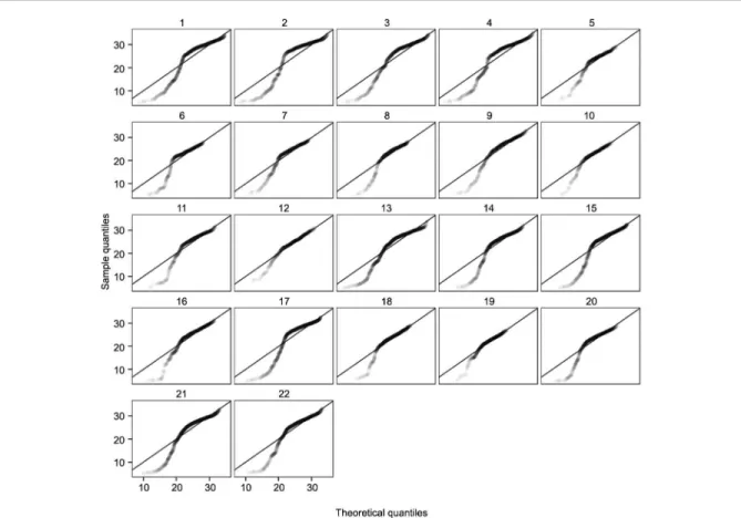
(lin-the best fit for (lin-the Weibull pdf in (lin-the canopy upper layer (Figure 3), partially due to crowns occluding the penetra-tion of laser beams at lower parts (Harding et al., 2001). The integration of terrestrial laser scanning (TLS) data with ALS-derived CHPs was presented as an alternative for improving canopy modeling at lower layers (Zhao et al., 2013).
The Weibull shape parameter (β_CHP) ranged from 5.7 to 11.3 confirming the negative asymmetry ob-served in the histograms of Figure 2 (Table 2). All the ALS metrics except β_CHP were positively correlated with the stem biomass. The metric P10 did not present strong correlation with the stem biomass, and it was ex-cluded from further analysis (Table 3).
ear regression and ordinary kriging) to visually compare results with one former basal area map obtained from a census of DBH on Feb 2008 (Campoe et al., 2012). To our knowledge, no study has yet compared the quality of stem biomass maps generated from regression with ALS data and generated from ordinary kriging of field-derived data, in even-aged eucalypt plantations.
Results
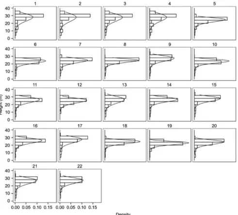
All plots presented negatively skewed data, and considerable variability between plots (Figure 2). On av-erage, 88 % of the laser points were observed above a height of 20 meters. The quantile-quantile plot showed
Figure 2 – Apparent eucalypt canopy height profiles (CHPs) per training plot. The vertical axis shows the laser point heights and the horizontal axis is the probability density of occurrence in each height class. The solid lines are the Weibull probability density functions fitted to the observed airborne laser scanning (ALS) data (histograms).
Table 2 – Summary of metrics resulted from processing the airborne laser scanning data (ALS) data of the 22 training plots in the eucalypt plantation site.
Stat. α_CHP β_CHP P10 P30 P70 P90 Mean St. dev. Variance p_understory
- m - --- m --- m² %
min 23.4 5.7 18.6 21.9 23.8 25.0 22.4 2.8 8.0 4.0
avg. 26.6 8.4 20.8 25.1 27.6 29.0 25.4 4.4 20.1 10.7
max 28.9 11.3 24.4 28.0 30.7 32.2 27.7 6.0 36.4 16.5
st. dev. 1.7 1.6 1.4 1.8 2.1 2.1 1.6 0.9 8.3 3.7
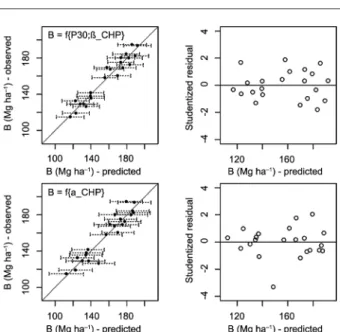
The best model resulted from using the explanatory P30 variable combined with β_CHP (adj. R² = 0.93), since using the P30 alone had already yielded a good fit (adj. R² = 0.91). It was already expected that height metrics would have greater explanatory power than metrics of height dispersion (Bouvier et al., 2015). The metric p_un-derstory had only moderate correlation with the stem bio-mass (adj. R² = 0.5) and no interaction effect with other ALS metrics was observed. On the other hand, there was an improvement issue when α_CHP was combined with the field-derived statistic density of stems (adj. R² = 0.89 to adj. R² = 0.92). No improvements were noted through using the natural logarithm of the stem biomass (Table 3). The observed and predicted values for the stem bio-mass regressed on P30 and β_CHP (model 1) and on α_CHP (model 2) are shown in Figure 4. The observations close to the 1:1 diagonal indicate a good model fit. This was also corroborated by the leave-one-out cross validation, which demonstrated rRMSE to be equal to 5 % for both models.
Figure 5 shows the Gaussian semivariogram for the stem biomass constructed from the training dataset. The model presented a nugget effect equal to 128 (Mg ha−1)2 and a sill equal to 1129 (Mg ha−1)2 at a range of 574 m. The leave-one-out-cross validation from the ordinary kriging resulted in an rRMSE equal to 13 %, which was 160 % greater than the regression models.
Figure 3 – Quantile-quantile plot per training plot. The vertical axis shows the sample quantiles for laser point heights and the horizontal axis illustrates the Weibull distribution quantiles.
Table 3 – Eucalypt stem biomass models dependent on airborne laser scanning (ALS) metrics. The values between parentheses represent the standard error of the parameters.
# Model adj.R² AIC VIF
1 B = -287.3 + 16.2*P30 + 4.3*β_CHP 0.93 151.1 3.43 (49.4) (1.5) (1.7)
2 B = -207.2 + 13.7*α_CHP 0.89 159.8 (27.63) (1.03)
3 B = 254.0 - 11.6*β_CHP 0.5 193.4
(20.9) (2.5)
4 B = 104.9 + 4.9*p_understory 0.5 193.5 (11.8) (1.0)
5 ln(B) = -3.9 + 2.6*ln(P30) + 0.16*sqrt(β_CHP) 0.93 -71.6 3.33 (0.88) (0.23) (0.06)
6* ln(B) = 2.9 + 0.09*P30 0.91 -65.6 (0.15) (0.006)
7* ln(B) = 4.6 + 0.1*P30 - 0.7*ln(P90) ns
0.91 -64.8 22.4 (1.6) (0.03) (0.67)
8* ln(B) = 2.6 + 0.09*Mean + 0.0002* sqrt(P70) ns
0.89 -60.9 40.4 (0.86) (0.04) (0.38)
9 B = -304.1 + 14.5*α_CHP + 0.05*stem.density 0.92 153.4 1.1 (40.1) (0.9) (0.02)
The predictions from the regression models showed slightly higher correlation with the validation dataset than the ordinary kriging (ρ = 0.8, ρ = 0.82, and
ρ = 0.71, respectively, Figure 6). The result is coherent with the work of Meng et al. (2009), who studied differ-ent methods of kriging to estimate the basal area in pine forests in the state of Georgia, USA. They found that applying regression kriging using Landsat ETM+ data as the auxiliary variable improved the results compared to ordinary kriging interpolation (R2 = 0.9 and R2 = 0.75, respectively).
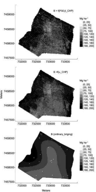
The map of the stem biomass generated from the metrics P30 and β_CHP were shown to be sensitive to the overlapping effect along adjacent flight lines (pixels scattered in the northwest-southeast direction) (Figure 7).
All maps show the gradient of productivity simi-lar to that described by Campoe et al. (2012); i.e., lower elevations in the terrain had higher stem biomass stock than the highest locations. However, the maps differed considerably in relation to local spatial patterns. A visual validation with the collinear variable of the stem bio-mass, basal area, is shown in Figure 8.
Discussion
There was great variability between the observed apparent canopy height profiles (CHPs), even though all trees in the stand are about the same age. The CHP is a signature of the forest structure, and is useful in a variety of contexts, like monitoring spatial and tempo-ral changes (Coops et al., 2007), mapping homogeneous strata (Nelson et al., 2003), and identifying vegetation types (Harding et al., 2001; Jaskierniak et al., 2011). Dean et al. (2009) were able to retrieve DBH values in a 36-year-old even-aged loblolly pine (Pinus taeda L.) stand from variable height to the base of live crown and height to crown median, which were retrieved from ALS-de-rived CHPs (n = 17, R2 = 0.97).
The ALS metric P30 presented the greatest cor-relation with stem biomass. d’Oliveira et al. (2012) observed a similar correlation between the height
per-Figure 4 – Eucalypt stem biomass (B) regressed on P30 and β_CHP (model 1, from Table 3) in the upper layer and regressed on α_CHP (model 2) in the lower layer. The horizontal bars in the left column represent the prediction intervals with 95 % confidence level.
Figure 5 – Gaussian semivariogram of eucalypt stem biomass built from the training dataset. The points represent the number of observed pairs in class k.
tical foliage profile from a hinoki stand (Chamaecyparis obtusa (Sieb. et Zucc.) Endl.) in central Japan. The im-provement from adding the field-derived variable den-sity of trees together with α_CHP seems to be promising owing to the potential of ALS data to quantify trees at the stand level (Görgens et al., 2015b; Popescu et al., 2003; Oliveira et al., 2012).
The shape parameter of the Weibull distribution (β_CHP) was the only ALS metric negatively correlat-ed with stem biomass. This result was also observcorrelat-ed in Coops et al. (2007) in relation to the DBH variable in different mixed stands of Vancouver Island, Canada. The Weibull pdf shape parameter is related to the degree of data dispersion in the distribution. With the scale pa-rameter fixed, the greater the value of the shape param-eter, the smaller the curve width at the mode. In models where β_CHP was used together with P30, there was a mediation effect; i.e., β_CHP correlated positively with stem biomass. The hypothesis is that for similar canopy height layers, a smaller vertical dispersion of heights is indicative of homogeneity, which would lead to more productive stands (Stape et al., 2010).
The ALS metric p_understory showed only moder-ate correlation with stem biomass and did not capture the variation in the forest horizontal structure as ex-pected. This is because the most productive plots also had more ALS points intercepted by the crown, thereby underestimating the density of trees in the understory layer. Additionally, observations were influenced by the point density heterogeneity within the ALS data, par-tially created by the overlapping of swaths during the flight (Bater et al., 2011; Görgens et al., 2015a). The se-lected regression models had at most two explanatory variables, and they were able to explain 93 % of the stem biomass variation. Stephens et al. (2012) explained 70 % of total carbon stock in forests of New Zealand with just one ALS height metric, observing that the addition of a density metric slightly improved the quality of the model (2 %), but a third variable did not bring any im-provement.
Figure 8 – Eucalypt basal area (G) maps. The map in the center is generated from a census of diameter at breast height (DBH) when the forest was 5.3 years old. The map on the left is G regressed on α_CHP, while the map on the right was derived from ordinary kriging interpolation.
Figure 7 – Eucalypt stem biomass prediction maps. In the upper and middle layer are linear regression models 1 and 2, from Table 3. The lower layer was derived from ordinary kriging interpolation (the white dots represent the training plots location).
ver-The stem biomass maps constructed from the linear models with ALS metrics and from the ordinary kriging interpolation were consistent with the existing gradient of productivity shown by Campoe et al. (2012). However, we observed from the validation statistics and visual inspection that the regression models fitted from the ALS metrics (P30 and α_CHP) generated more real-istic maps, corroborating the initial hypothesis.
Acknowledgments
This paper is part of the research program devel-oped by GET-LiDAR (http://cmq.esalq.usp.br/getlidar/ doku.php). We acknowledge the following institutions for their support in providing the laser and field datas-ets: the Eucflux project (http://www.ipef.br/eucflux/en/), Esteio Engenharia e Aerolevantamentos S.A., Duratex S.A., Forestry Science and Research Institute (IPEF), North Carolina State University (NCSU), and Virginia Polytechnic Institute and State University (VT). We also thank two anonymous reviewers whose suggestions helped to improve this manuscript.
References
Alvares, C.A.; Stape, J.L.; Sentelhas, P.C.; Gonçalves, J.L.M.; Sparovek, G. 2013. Köppen’s climate classification map for Brazil. Meteorologische Zeitschrift 22: 711-728.
Baltsavias, E.P. 1999. Airborne laser scanning: basic relations and formulas. ISPRS Journal of Photogrammetry and Remote Sensing 54: 199-214.
Bater, C.W.; Wulder, M.A.; Coops, N.C.; Nelson, R.F.; Hilker, T.; Næsset, E. 2011. Stability of sample-based scanning-LiDAR-derived vegetation metrics for forest monitoring. IEEE Transactions on Geoscience and Remote Sensing 49: 2385-2392.
Bouvier, M.; Durrieu, S.; Fournier, R.A.; Renaud, J. 2015. Generalizing predictive models of forest inventory attributes using an area-based approach with airborne LiDAR data. Remote Sensing of Environment 156: 322-334.
Campoe, O.C.; Stape, J.L.; Laclau, J.P.; Marsden, C.; Nouvellon, Y. 2012. Stand-level patterns of carbon fluxes and partitioning in a Eucalyptus grandis plantation across a gradient of productivity, in Sao Paulo state, Brazil. Tree Physiology 32: 696-706. Campos, J.C.C.; Leite, H.G. 2013. Forest Mensuration: Questions
and Answers = Mensuração Florestal:Perguntas e Respostas.
4ed. Editora UFV, Viçosa, MG, Brazil (in Portuguese).
Cohen, A.C. 1965. Maximum likelihood estimation in the weibull distribution based on complete and on censored samples. Technometrics 7: 579-588.
Coops, N.C.; Hilker, T.; Wulder, M.A.; St-Onge, B.; Newnham, G.; Siggins, A.; Trofymow, J.A.T. 2007. Estimating canopy structure of Douglas-fir forest stands from discrete-return LiDAR. Trees 21: 295-310.
Dean, T.J.; Cao, Q.V.; Roberts, S.D.; Evans, D.L. 2009. Measuring heights to crown base and crown median with LiDAR in a mature, even-aged loblolly pine stand. Forest Ecology and Management 257: 126-0133.
d’Oliveira, M.V.N.; Reutebuch, S.E.; McGaughey, R.J.; Andersen, H.E. 2012. Estimating forest biomass and identifying low-intensity logging areas using airborne scanning lidar in Antimary State Forest, Acre state, western Brazilian Amazon. Remote Sensing of Environment 124: 479-491.
Evans, J.S.; Hudak, A.T. 2007. A Multiscale curvature algorithm for classifying discrete return LiDAR in forested environments. IEEE Transactions on Geoscience and Remote Sensing 45: 1029-1038.
Fox, J.; Monette, G. 1992. Generalized collinearity diagnostics. Journal of the American Statistical Association 87: 178-183. Gonçalves, J.L.M.; Alvares, C.A.; Higa, A.R.; Silva, L.D.; Alfenas,
A.C.; Stahl, J.; Ferraz, S.F.B.; Lima, W.P.; Brancalion, P.H.S.; Hubner, A.; Bouillet, J.P.D.; Laclau, J.P.; Nouvellon, Y.; Epron, D. 2013. Integrating genetic and silvicultural strategies to minimize abiotic and biotic constraints in Brazilian eucalypt plantations. Forest Ecology and Management 301: 6-27. Görgens, E.B.; Packalen, P.; Silva, A.G.P.; Alvares, C.A.; Campoe,
O.C.; Stape, J.L.; Rodriguez, L.C.E. 2015a. Stand volume models based on stable metrics as from multiple ALS acquisitions in Eucalyptus plantations. Annals of Forest Science 72: 489-498. Görgens, E.B.; Rodriguez, L.C.E.; Silva, A.G.P.; Silva, C.A. 2015b.
Individual tree identification in airborne laser data by inverse search window. Cerne 21: 91-96 (in Portuguese, with abstract in English).
Harding, D.J.; Lefsky, M.A.; Parker, G.G.; Blair, J.B. 2001. Laser altimeter canopy height profiles: methods and validation for closed-canopy, broadleaf forests. Remote Sensing of Environment 76: 283-297.
Hiemstra, P.H.; Pebesma, E.J.; Twenhöfel, C.J.W.; Heuvelink, G.B.M. 2009. Real-time automatic interpolation of ambient gamma dose rates from the Dutch radioactivity monitoring network. Computers and Geosciences 35: 1711-1721.
Hummel, S.; Hudak, A.T.; Uebler, E.H.; Falkowski, M.J.; Megown, K.A. 2011. A comparison of accuracy and cost of LiDAR versus stand exam data for landscape management on the Malheur National Forest. Journal of Forestry 109: 267-273.
Jaskierniak, D.; Lane, P.N.J.; Robinson, A.; Lucieer, A. 2011. Extracting LiDAR indices to characterise multilayered forest structure using mixture distribution functions. Remote Sensing of Environment 115: 573-585.
Lefsky, M.A.; Cohen, W.B.; Acker, S.A.; Parker, G.G.; Spies, T.A.; Harding, D. 1999. LiDAR remote sensing of the canopy structure and biophysical properties of Douglas-Fir western hemlock forests. Remote Sensing of Environment 70: 339-361.
Le Maire, G.; Marsden, C.; Verhoef, W.; Ponzoni, F.J.; Seen, D.L.; Bégué, A.; Stape, J.L.; Nouvellon, Y. 2011. Leaf area index estimation with MODIS reflectance time series and model inversion during full rotations of Eucalyptus plantations. Remote Sensing of Environment 115: 586-599.
Lovell, J.L.; Jupp, D.L.B.; Culvenor, D.S.; Coops, N.C. 2003. Using airborne and ground-based ranging lidar to measure canopy structure in Australian forests. Canadian Journal of Remote Sensing 29: 607-622.
Magnussen, S.; Boudewyn, P. 1998. Derivations of stand heights from airborne laser scanner data with canopy-based quantile estimators. Canadian Journal of Forest Research 1031: 1016-1031.
Magnussen, S.; Eggermont, P.; LaRiccia, V.N. 1999. Recovering tree heights from airborne laser scanner data. Forest Science 45: 407-422.
Maltamo, M.; Eerikäinen, K.; Pitkänen, J.; Hyyppä, J.; Vehmas, M. 2004. Estimation of timber volume and stem density based on scanning laser altimetry and expected tree size distribution functions. Remote Sensing of Environment 90: 319-330. McCool, J.I. 2012. Using the Weibull Distribution: Reliability,
Modeling and Inference. John Wiley, Hoboken, NJ, USA. Meng, Q.; Cieszewski, C.; Madden, M. 2009. Large area forest
inventory using landsat ETM+: a geostatistical approach. ISPRS Journal of Photogrammetry and Remote Sensing 64: 27-36
Mori, S.; Hagihara, A. 1991. Crown profile of foliage area characterized with the Weibull distribution in a hinoki (Chamaecyparis obtusa) stand. Trees 5: 149-152.
Næsset, E. 1997. Estimating timber volume of forest stands using airborne laser scanner data. Remote Sensing of Environment 61: 246-253.
Næsset, E. 2002. Predicting forest stand characteristics with airborne scanning laser using a practical two-stage procedure and field data. Remote Sensing of Environment 80: 88-99. Nelson, R.; Valenti, M.A.; Short, A.; Keller, C. 2003. a multiple
resource inventory of Delaware using airborne laser data. BioScience 53: 981-992.
Nyström, M.; Holmgren, J.; Olsson, H. 2012. Prediction of tree biomass in the forest–tundra ecotone using airborne laser scanning. Remote Sensing of Environment 123: 271-279. Oliveira, L.T.; Carvalho, L.M.T.; Ferreira, M.Z.; Oliveira, T.C.A.;
Acerbi Junior, F.W. 2012. Application of LiDAR to forest inventory for tree count in stands of Eucalyptus sp. Cerne 18: 175-184.
Packalén, P.; Mehtätalo, L.; Maltamo, M. 2011. ALS-based estimation of plot volume and site index in a eucalyptus plantation with a nonlinear mixed-effect model that accounts for the clone effect. Annals of Forest Science 68: 1085-1092. Picard, R.R.; Cook, R.D. 1984. Cross-validation of regression
models. Journal of the American Statistical Association 79: 575-583.
Popescu, S.C.; Wynne, R.H.; Nelson, R.F. 2003. Measuring individual tree crown diameter with liDAR and assessing its influence on estimating forest volume and biomass. Canadian Journal of Remote Sensing 29: 564-577.
Reutebuch, S.E.; Andersen, H.E.; McGaughey, R.J. 2005. Light detection and ranging (LIDAR): an emerging tool for multiple resource inventory. Journal of Forestry 103: 286-292.
Silva, C.A.; Klauberg, C.; Carvalho, S.P.C.; Hudak, A.T.; Rodriguez, L.C.E. 2014. Mapping aboveground carbon stocks using LiDAR data in Eucalyptus spp. plantations in the state of São Paulo, Brazil. Scientia Forestalis 42: 591-604.
Stape, J.L.; Binkley, D.; Ryan, M.G.; Fonseca, S.; Loos, R.A.; Takahashi, E.N.; Silva, C.R.; Silva, S.R.; Hakamada, R.E.; Ferreira, J.M.A.; Lima, A.M.N.; Gava, J.L.; Leite, F.P.; Andrade, H.B.; Alves, J.M.; Silva, G.G.C.; Azevedo, M.R. 2010. The Brazil Eucalyptus Potential Productivity Project: influence of water, nutrients and stand uniformity on wood production. Forest Ecology and Management 259: 1684-1694.
Stephens, P.R.; Kimberley, M.O.; Beets, P.N.; Paul, T.S.H.; Searles, N.; Bell, A.; Brack, C.; Broadley, J. 2012. Airborne scanning LiDAR in a double sampling forest carbon inventory. Remote Sensing of Environment 117: 348-357.
Vauhkonen, J.; MehtÄtalo, L.; Packalén, P. 2011. Combining tree height samples produced by airborne laser scanning and stand management records to estimate plot volume in Eucalyptus plantations. Canadian Journal of Forest Research 41: 1649-1658.
Viana, H.; Aranha, J.; Lopes, D.; Cohen, W.B. 2012. Estimation of crown biomass of Pinus pinaster stands and shrubland above-ground biomass using forest inventory data, remotely sensed imagery and spatial prediction models. Ecological Modelling 226: 22-35.
Zhao, F.; Yang, X.; Strahler, A.H.; Schaaf, C.L.; Yao, T.; Wang, Z.; Román, M.O.; Woodcock, C.E.; Ni-Meister, W.; Jupp, D.L.B.; Lovell, J.L.; Culvenor, D.S.; Newnham, G. J.; Tang, H.; Dubayah, R.O. 2013. A comparison of foliage profiles in the Sierra National Forest obtained with a full-waveform under-canopy EVI lidar system with the foliage profiles obtained with an airborne full-waveform LVIS lidar system. Remote Sensing of Environment 136: 330-341.
Zhou, J.; Proisy, C.; Descombes, X.; le Maire, G.; Nouvellon, Y.; Stape, J.L.; Viennois, G.; Zerubia, J.; Couteron, P. 2013. Mapping local density of young Eucalyptus plantations by individual tree detection in high spatial resolution satellite images. Forest Ecology and Management 301: 29-141.