Probabilistic Analysis of Pattern Formation in
Monotonic Self-Assembly
Tyler G. Moore1*, Max H. Garzon1, Russell J. Deaton2
1Department of Computer Science, University of Memphis, Memphis, TN, United States of America, 2Department of Electrical Engineering and Computer Engineering, University of Memphis, Memphis, TN,
United States of America
Abstract
Inspired by biological systems, self-assembly aims to construct complex structures. It func-tions through piece-wise, local interacfunc-tions among component parts and has the potential to produce novel materials and devices at the nanoscale. Algorithmic self-assembly models the product of self-assembly as the output of some computational process, and attempts to control the process of assembly algorithmically. Though providing fundamental insights, these computational models have yet to fully account for the randomness that is inherent in experimental realizations, which tend to be based on trial and error methods. In order to develop a method of analysis that addresses experimental parameters, such as error and yield, this work focuses on the capability of assembly systems to produce a pre-determined set of target patterns, either accurately or perhaps only approximately. Self-assembly sys-tems that assemble patterns that are similar to the targets in a significant percentage are
“strong”assemblers. In addition, assemblers should predominantly produce target patterns,
with a small percentage of errors or junk. These definitions approximate notions of yield and purity in chemistry and manufacturing. By combining these definitions, a criterion for effi-cient assembly is developed that can be used to compare the ability of different assembly systems to produce a given target set. Efficiency is a composite measure of the accuracy and purity of an assembler. Typical examples in algorithmic assembly are assessed in the context of these metrics. In addition to validating the method, they also provide some insight that might be used to guide experimentation. Finally, some general results are established that, for efficient assembly, imply that every target pattern is guaranteed to be assembled with a minimum common positive probability, regardless of its size, and that a trichotomy exists to characterize the global behavior of typical efficient, monotonic self-assembly sys-tems in the literature.
Introduction
Self-assembly is a process by which self-directed systems gain complexity over time through the local interactions of their simple components, and is a fundamental and pervasive process OPEN ACCESS
Citation:Moore TG, Garzon MH, Deaton RJ (2015) Probabilistic Analysis of Pattern Formation in Monotonic Self-Assembly. PLoS ONE 10(9): e0137982. doi:10.1371/journal.pone.0137982
Editor:Ming Dao, Massachusetts Institute Of Technology, UNITED STATES
Received:December 26, 2014
Accepted:August 25, 2015
Published:September 30, 2015
Copyright:© 2015 Moore et al. This is an open access article distributed under the terms of the
Creative Commons Attribution License, which permits unrestricted use, distribution, and reproduction in any medium, provided the original author and source are credited.
Data Availability Statement:All relevant data are within the paper.
Funding:This work was supported by the National Science Foundation atwww.nsf.govthrough
“EAGER: Self-Assembly of Complex Systems” (CCF-1049719) and“Engineering Nano-Building Block Toolboxes for Programmable Self-Assembly of Nanostructures with Arbitrary Shapes and Functions”
(CMMI-1235100). The funders had no role in study design, data collection and analysis, decision to publish, or preparation of the manuscript.
in natural phenomena including membrane formation and protein folding. In experimental self-assembly, systems are designed to execute an algorithm that is implemented through spe-cific local interactions, for example, DNA template matching reactions. Study of the self-assembly of DNA-based nanostructures started with seminal work by Ned Seeman, Erik Win-free, Chad Mirkin, and others [1,2]. DNA continues to be a promising material for construc-tion of nanoscale structures and devices [3–11]. Other than DNA, diblock copolymers [12] and patchy particles [13] provide alternate mechanisms for algorithmic self-assembly. Although the results in this paper are potentially applicable to other systems, the focus here is on mono-tonic algorithmic self-assembly where stably bound components do not detach from the grow-ing assembly.
The design of nanostructures and their experimental realizations have been mainlyad hoc or trial and error. In the lab, self-assembly is subject to incomplete reactions, binding errors, kinetic trapping, and other inevitable random effects. The result is that the desired, target struc-tures are often lost in byproducts (junk) of the assembly process. Though revealing interesting capabilities of assembly systems, theoretical models have focused on the algorithmic power and properties of theprocessof assembly that are necessary to produce unique and exact target patterns. Therefore, there exists a disconnect between experimental practice, and theoretical models and results of algorithmic self-assembly.
In this paper, a probabilistic method of analysis to characterize how well self-assembly sys-tems produce sets of target patterns is proposed. The method is not an attempt to model proba-bilistic mechanisms during growth, as in Chandranet al.’s probabilistic tile assembly model [14] or Cooket al.’s Markov chains [15]. Rather, it focuses on the relationship between the sets of intended target and actually assembled patterns. The targets are what the designer or experi-mentalist wants to be assembled, and the quality of an assembly system is measured by its abil-ity to accurately construct the target set. Thus, strong assemblers should construct patterns that resemble target patterns, as well as produce a reasonable fraction of the target set. In addi-tion, assemblers should make target patterns with a limited amount of impurities (or junk). Assembly systems that have both these properties are termedefficient. The strength and effi-ciency of assembly should depend not only on the assembly system, but also on the set of target patterns.
Probabilistic analysis is concerned with the overall behavior of pattern formation by the assembly system, regardless of the system’s primary components, model of interaction, or the particulars of the growth process. One can run a probabilistic analysis to compare the perfor-mance of two assembly systems on a given target set, even if one or both of them are determin-istic, nondetermindetermin-istic, and/or probabilistic. Although the approach suggested is quite general and applies to many types of assembly systems, the focus here is on algorithmic self-assembly systems that produce target patterns with a degree of nondeterminism. No particular assump-tion is made on the nature of this nondeterminism, which may range from errors due to experi-mental implementation of a model, such as stochastic or nondeterministic binding, to kinetic effects, or flexibility in the properties sought in the assembled patterns. The method might pro-vide experimenters with a guide to choose assemblers that are more experimentally feasible. The method captures several notions of yield of an assembly process, as well as assemblers that are, borrowing from Valiant’s theory of the learnable [16],“probably approximately correct”.
not require cooperation [17] shows that noncooperative assembly systems are efficient. When cooperation is necessary to form target patterns, then, any degree of cooperation is more effi-cient than none at all. For example, in the formation of computational structures like binary counters, potential noncooperative binding results in assemblers that are not efficient. In addi-tion, the requirements of efficiency impose limits on the uncontrolled accretion of components that may be addressed by constraining the assembly of patterns to finite areas or geometries that simulate experimentally accessible parameters, such as relatively small concentrations of reactants or small, fixed-size reaction vessels. Finally, some general results follow from the defi-nitions of the method. For efficient assemblers, target patterns are assembled with positive probability independently of the dynamics of the assembler, and the dynamic behavior of a good assembler can be qualitatively characterized or estimated solely from the estimates of or bounds on its efficiency.
The layout of the paper is as follows. Some necessary background information is given in section 1. Section 2 provides precise definitions of the requisite concepts and discusses the pre-cise characterizations of desirable properties such as“strength”,“purity”, and“efficiency”. Examples in section 3 are then presented of analyses of typical systems in self-assembly, some with respect to implementations under plausible error conditions. Section 3 then presents gen-eral results on probabilistic analysis concerning efficiency, as previously characterized. In the final section we provide some discussion and raise a few questions of interest arising from this approach to self-assembly.
Background
The field of algorithmic self-assembly attempts to understand this process through models of molecular programs for the production of nanomaterials with complex structures, properties, and functionalities. Among the earliest and best known models is the abstract Tile Assembly Model (aTAM). Tile types are assigned four labels that abstract the bonding mechanism to the matching of labels or glues that color the sides of tiles [18,19]. Growth of the assembly pro-ceeds sequentially starting from some set of“seed”tiles. Tiles are attached to the growing assembly only if the glue strength of matching tile edges exceeds some designated“ tempera-ture”τ. Thus, temperature is an abstraction of the minimum energy required for bonding
between tiles. Recently, an equivalent structure was formed by conjugating DNA oligonucleo-tides at right angles on the surface of a gold nanoparticle [20]. The model demonstrates that cooperative self-assembly processes operating atτ= 2 are at least as complex as arbitrary
com-putation by programs equivalent to Turing machines. This property is referred to as computa-tion universality [1,21]. On the other hand, the assembly power of the model at temperatureτ
= 1 remains unknown [15], but is suspected not to be universal. From an experimental point of view, however, tile assembly atτ= 1 is considered to have advantages, such as speed and ease
of implementation. Recent work has also proved that cooperative models are intrinsically uni-versal [22],i.e., that there exist certain tile assembly systems that are capable of assembling sim-ulations of any other tile assembly system in the model, up to a re-scaling factor.
The notation for the TAM is taken from [15,18,19,23]. A tile typetis a“Wang”tile with glues (labels)σ2Sassigned to its 4 edges,σN(t),σE(t),σS(t),σW(t), corresponding to North,
East, South, and West, from some alphabetS. A tile assembly system is a tripleT= (T,s,τ),
whereTis a set of tile types,sTis a set of seed or initial tiles, andτis a temperature. In
addition, there is the glue functiong:S×S!Z+[0 that evaluates the bonding strength of
pairs of glues. An assemblyαcan then be described as a mapping from the integer latticeZ2
Usually, tile self-assembly takes place on the 2D square lattice or grid,Z2, and temperatures
are restricted toτ= 1 or 2. The assembly proceeds asynchronously and nondeterministically
with new tilest2Tattaching to eligible sites (i,j)2Z2ifαi,j=emptyandg(i,j,t)τ. An
assemblyα2A[T] is terminal if no tile can be added that is stable at temperatureτ(τ-stable).
The set of terminal assemblies isA◻[T]A[T]. An assembly sequence is calledlocally
deter-ministicif each new tile binds with strength exactlyτto the existing assembly, each eligible site
admits only one type of tile given that binding is allowed to occur only on pre-designated input labels on each tile type, and the the assembly sequence leads to a valid terminal assembly. A tile assembly system isdirectedif there is only one terminal assembly from any initial condition. If every assembly sequence associated with some tile assembly system is locally deterministic, then that tile assembly system is directed. An assembly sequence is a finite or infinite sequence of assemblies in which each assembly is a seed or is obtained from the previous one by the addi-tion of one tile. An example of a binary counter implemented with aτ= 2 tile set is shown in
Fig 1.
The family of tile assembly models includes a variety of other models, such as the 2-handed model or 2HAM [24] addressing unseeded arbitrary aggregation, the subsequent sTAM [25] in which tiles are given additional complexity and can react to local binding events, and the prob-abilistic pTAM [14]. Other models exist that account for the roles of kinetics [21], fuzzy tem-perature control [26], and global temperature scheduling and tile concentration programming [26–29] (see [30] for a survey). Other work has characterized the power of nondeterministic tile self-assembly to uniquely produce a single terminal assembly [31].
In addition to shedding light on the nature and complexity of the self-assembly process, tile assembly models are regularly used to analyze, predict and guide the results of molecular self-assembly in the laboratory. The kinetic Tile Assembly Model (kTAM) [21] is a nonmonotonic model of tile self-assembly that approximates the aTAM by controlling the forward rates (asso-ciation) and reverse rates (disso(asso-ciation) of tile types in the system. Other extensions of the aTAM allow for the robust and nearly optimal construction of a variety of unique terminal assemblies given a chance of error during aggregation using error-correcting and proofreading algorithms [32]. Despite this progress, tile assembly models have not fully addressed the role of errors in the assembly process, do not capture the intrinsic nondeterminism necessary for more realistic models or as seen in experimental nanofabrication, and have not completely explored the self-assembly power of other models, including noncooperative models of assem-bly [17,33].
As mentioned above, it is important to distinguish the type of probabilistic analysis in this paper from probabilistic models of self-assembly, where tiles attach with some probability based on the local context of the attachment. For example, the pTAM [14] is designed to show that tile assembly sets smaller than the Kolmogorov complexity of the set of patterns being assembled are possible, at the price of producing some undesirable patterns, and gives esti-mates of the probability of 1D assemblies of a fixed lengthNbeing constructed with tile sets of cardinalityO(log3N).
Patterns and Assemblers
Definition 1.Apatternx is a d-dimensional word over some alphabet∑(d>0). The size of
the patternjxjis a nonnegative integer number associated with every pattern x, such as the num-ber of unit squares/cubes in the corresponding region (its digital“area”or“volume”), the maxi-mum Manhattan distance of a cell in the support from a designated origin (also called the Manhattan radiusof the pattern), or the number of rows(height)or columns(width)in x.
An example of a 2D pattern is shown inFig 1. Ordinary words are defined up to rigid trans-lations in the 1D integer lattice where two words that only differ by a translation are considered to be identical. The situation is slightly more complicated in two and higher dimensions, par-ticularly in the context of tiling and self-assembly. An equivalent definition of size is a partition of the set of all possible patterns into layers, each consisting of all patterns of a particular size n0, regardless of the concept of size being used. We partition the set of patterns by size and, consistent with the aTAM, assume that patterns of sizenare obtained from patterns of sizen
−1 ornby adding some additional labeled units, so that patterns of size at mostnproperly
include those of size at mostn−1, for everyn0. In addition, patterns will be assumed to
snugly fit to the coordinate axes,i.e., their support must contain at least one unit square on each axis and they are entirely contained in the first quadrant/octant.
The object of study is a pattern assembler defined as any experimental process, mechanism or logical model that attempts to generate certain patterns from some initial conditions, possi-bly acting nondeterministically. Much attention has been given to analyzing the capabilities of the aTAM and other tiling models by designing assemblers that simulate deterministic compu-tations in order to ensure that the appropriate patterns will be error-free in the model. This work will focus on assemblers that will generally not produce patterns deterministically, or, even if deterministically, will produce patterns with a common set of features that characterize a possibly infinite family of target patterns. In general, the properties sought in the patterns of the target set may be dispersed throughout the patterns. Potentially desirable bulk properties of interest might include strength, conductivity, opacity, reflectivity, or plasmonic response. Other target properties include clusters of adjacent nonidentical labels (colorability), a ratio of one label to another (color mixing), and percolating subpatterns of active labels as discussed in Appendix A.
Fig 1. The binary counter tile set (Left) and a partial assembly (Right).The assembler counts from 0, represented asn-bits in the seed, by adding 1 to the previous layer up to the fulln-bit value 2n
−1.
Probabilistic Analysis
This section addresses the primary question: What is the appropriate definition of assembly of a target set of patternsPgiven that the assemblerGmay produce a set of patternsAthat poten-tially contains nontarget (or junk) patterns not inP? These two sets of interest are ideally the same, but in practice they may not be (Fig 2). At first, one might be tempted to require only thatGproduce a positive fraction of all patterns of every given sizen,i.e., to impose the condi-tion that for some fraccondi-tionp>0,
8n jAn\Pnj pjPnj; ð1Þ
whereAnandPndenote the set of patterns of sizeninAandP, respectively. A set of patternsP is weakly probabilistically assemblable if this condition holds for some assemblerGand some p>0. Thus, when an assemblerGweakly probabilistically assemblesPwith probabilityp= 1,
Gmust assemble all the target patterns of every sizen. In the aTAM, tile assembly systems are usually designed to implement an algorithm that produces the target setPwith probability p= 1 because the patterns assembled are all inPand all the target patterns are eventually gener-ated. In this case,A=P. In general, however, ConditionEq (1)is too weak to impose a hard constraint. For example, an assembler that produces every possible pattern of a given dimen-sion weakly assembles any target set of patternsPwith probabilityp= 1, since in that case An\Pn=Pn. Yet, the assembler has no idea what the set of target patterns is, so it will gener-ally produce an inordinate number of patterns not inPand cannot be considered“high yield”
or“efficient”. We also note that if one begins with any given assembler, it will likewise weakly assemble the full set of patterns it produces withp= 1 if the target set isfixed to be that seta posteriori. In contrast, an experimentalist wishing to self-assemble a product often has a partic-ular set of target patterns in mind before proceeding tofind an appropriate process in the lab to produce them. More desirable assemblers are expected not only to produce a significant frac-tion of the target set, but also to have some“idea”of what the target set of patterns is like. Therefore, we also require that no pattern produced be significantly different from all patterns of the same size in the target set. Such a concept can be obtained by adding a second condition as in Definition 3.
Strong and Efficient Probabilistic Pattern Formation
In order to evaluate the quality of an assembler, it is necessary to have a metric to quantify pat-tern similarity.
Definition 2.A pattern z is a subpattern of a given pattern x if its support is fully contained in the support of x (after an appropriate shift) and their tile labels match cell-wise. Given a frac-tion 0<p1, two patterns x and y of identical size n are said to be congruent modulo p,
denoted x*py, if and only if both contain a common subpattern z of size at least p × n (after an appropriate shift.)
Two patterns are thus congruent modulop= 1 if and only if they are identical. They are congruent mod1
2if they can be overlapped so that the labels of at least half of their unit cells match. Since every pair of patterns is congruent modulo 0, we assume thatp>0.
Definition 3.A pattern assemblerGprobabilistically assembles a given target set of patterns
Pwith respect to a notion of size n if and only if there exists a constant p>0 such that
8n jAn\Pnj pjPnj;
and
whereAn(Pn,respectively) denotes the set of patterns of size n assembled byG(contained inP,
respectively.) A set of patternsPis probabilistically assemblable if it is assembled with some prob-ability p>0 by some assemblerG.If so, the value p is then the strength of the assembler.
Informally, a (strong) probabilistic assembler has a good idea of the target set of patterns because every individual pattern it assembles captures a significant fractionpof some target pattern in the target set and because it captures a large fractionpof target patterns. A tightp can be regarded as the best common probability, across all sizes, of assembling a target pattern as compared to other target patterns. This value is different from the probability of assembling a target pattern with respect to the set of all assemblies, a matter that will be addressed in the next section. Note that an assemblerGprobabilistically assembles a target setPwithp= 1 only when every pattern assembled is a target pattern and every target pattern is assembled,i.e. if and only ifA=P. Thus we recover in this extreme case the usual notion of assembly used in the tile self-assembly literature, when restricting target patterns to terminal assemblies exclud-ing their partial assemblies. For example, aTAM assemblers are designed to produce the algo-rithmically assemblable target setPwith probabilityp= 1 because the patterns assembled are all inPand all the target patterns are eventually generated so thatA=P. However, implemen-tations of such systems for assemblers runin vitrousually do so withp<1 for large target sets.
Either some large fraction of patterns in the target set are not assembled perfectly, or the assem-bler produces some patterns that do not match closely with any pattern in the target set. Thus ifPis regarded as the theoretically ideal stoichiometric yield, then,pcan be regarded as an abstraction of the chemical reaction notion of“yield.”
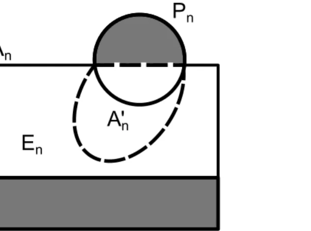
In order to address the production of undesirable (or“junk”) patterns outside the target set P, a bound is placed on the fraction of nontarget patterns assembled. The set of assembled pat-terns of every sizenis comprised of three characteristic subsets, namely the target patterns already assembled (An\Pn), the promising patterns that will eventually become targets with further assembly (A0n ðAn\PnÞ), and the erroneous or junk patterns (An A
0
n) that never
will (Fig 2).
Definition 4.Given a pattern assemblerGfor a set of target patternsP,an assembled pattern of size n>0 is called a promising pattern if it is either a target pattern itself or it will eventually become a target pattern by valid further assembly on it as a seed. The set of these patterns is
Fig 2. The three characteristic sets of assemblies in an assembly system.The set of assembled patternsAncontains some target patterns (An\Pn) that are already assembled, the set of promising patterns
A0
nthat includesAn\Pnas well as nontarget patterns that will eventually become target patterns of larger
denotedA0n.Otherwise it is nonpromising, erroneous or an assembly error.Endenotes the set of erroneous assemblies.
For every sizen, the set of erroneous patternsEn¼An A
0
nwill never become targets and
are thus“junk”produced by an assembler relative to the set of target patterns. It is clear that recognizing the set of promising patterns associated with some pattern assembler is, in general, not recursively solvable even in the aTAM. Often however, for physical systems, the concern is not just with the system’s ability to produce target patterns, but also with its ability to guarantee that the number of unavoidable error patterns produced by the assembly process is small rela-tive to the target product.
Definition 5.A set of patternsPis calledassemblable with impurityq if there exists some assemblerGand constant q>0 such that
8n0; jE
nj ¼ jAn A
0
nj qjPnj
IfPis both probabilistically assemblable by an assemblerGwith strength p and impurity q, the inverse1
qis called the purity and the ratio E¼ p
qis called theefficiencyofG.The setPisefficiently
probabilistically assemblableif it is assemblable by some assembler with efficiency E¼p q>1.
A tight suchqcharacterizes how conservative the assembler is in forming patterns in the target set by bounding the size of the set of error patterns assembled with respect to the size of the target set. It can be regarded as the worst-case fraction, across all sizes, of assembled error patterns in relation to the set of target patterns. As mentioned above, efficiency metrics allow the comparison of the relative efficiency of two assemblers to produce a given target set.
Strictly speaking, Definitions 3–5 require a proper concept of assembler. However, we will abstain from a general definition because our analysis specifically applies to a number of well-known models and experimental techniques in nanoscale self-assembly, as described below. Moreover, we believe the framework is adaptable to other models not discussed herein. Although the definitions apply to assemblers in models that are nonmonotonic (such as the aTAM with negative strength glues [34]), the analyses become more complex, and so this work is mostly concerned with monotonic systems where tile detachment is not allowed.
Examples
Next, several examples demonstrate the method of probabilistic analysis. Like complexity anal-ysis of algorithms, probabilistic analanal-ysis of an assembler requires that a target to be assembled is chosen first, as well as a concept of pattern sizen. The analysis requires estimation of thep’s andq’s,i.e., the worst-case probability of assembly strength and impurity in the assembled pat-terns, across all possible sizesn. The relative performance of different assemblers to realize the target set can then be compared using these measures. In addition, to investigate the effect of errors, we examine the extreme cases of perfect cooperativity or none.
While there exists target patterns that cannot be assembled by any noncooperative aTAM assembler [35], the cooperative aTAM is a powerful model for the algorithmic assembly of unique patterns. We begin with an analysis of the canonical cooperative aTAM assemblerℬc, a
binary counter [23].Fig 1shows the tile set and a partial assembly. The target set consists of 2D patterns producible from a single seed (representing 0 written innbits) and enumerating in increasing order all binary numbers with up to the same number of bits. Thus, the target set is infinite,jPnj>0 for alln>0. The size of a pattern is the Manhattan radius of the pattern’s sup-port taken from the seed at the origin (lower left corner.) Cooperative aTAM assemblers are capable of universal computation [21] and counting requires only the operation of addition by one (a local operation.) Therefore, assembly systemℬcis capable of producing this target
set algorithmically. First, by some valid assembly sequences,ℬ
pattern in the target set; therefore,A\P=P. Second, patterns of Manhattan radiusn assem-bled byℬ
cmatch perfectly with at least one pattern of radiusnin the target set, sinceℬc cor-rectly assembles the patterns of partial binary numbers and the target set includes all such patterns of the same radius. Thereforeℬ
cprobabilistically assemblesPwith probabilityp= 1. We analyze the impurity of this assembler by first counting the size ofAn A
0
n,i.e. we
com-pute the number of junk patterns assembled byℬ
c. In this case,jAn A
0
nj ¼0. We again refer
to the algorithmic construction and note that no tile can be placed in error in the model. There-fore,ℬcprobabilistically assemblesPwith perfect purity (anyq>0 will do) and arbitrarily
large efficiencyE.
Now let us consider an assemblerℬeidentical toℬcexcept that it is run at temperatureτ=
1. Tiles can now attach if only one glue matches an open edge, so the assembly is noncoopera-tive. Thus, in contrast with the idealℬcatτ= 2, this case ofτ= 1 represents the other extreme
of error-prone assembly. Although the targets are still assembled weakly withp= 1, many other nontarget patterns are now assembled that can have an arbitrarily small number of cells in common with any target pattern of the same size. For each larger size, the proportion of common tiles decreases to arbitrarily small values as the number of bits and radius increase. Therefore, the strength of the assembler cannot be any positivep>0. Likewise, an arbitrarily
large fraction of assembled patterns of sizenare not target patterns, so that the impurityqalso deteriorates (requiring larger and larger values forq.) Therefore, because the junk grows much faster than the target patterns asnincreases, the assembler effectively has efficiencyE= 0. We remark that similar probabilistic analyses are obtained for other systems deterministically pro-ducing unique shapes or finite sets of patterns, such as squares [18].
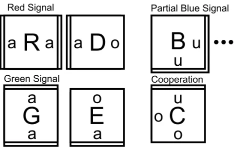
The second example, dubbed the RGB assembler (Fig 3), was designed to emphasize issues associated with nondeterminism, cooperative binding, and the effects of finite reaction spaces or numbers of reactants. In a variant aTAM, the assembly space is bounded by a given square seed of side sizeLwith a designated point of cooperation at (L/2,L/2) in the support. This frame is an abstraction that represents the effects of a finite-sized reaction vessel and limited numbers of reactants. The RGB assembler is designed to nondeterministically grow two signals, one red from gate R and one green from gate G, towards a point of cooperation C. If and when C is reached, another signal is produced from C that reports successful cooperation at a certain site B. Minimal cooperation at a single site C is required to nondeterministically produce and record a logical AND signal at an output location B from given seed input signals R and G, all three located on the perimeter of the tiling area, as illustrated inFig 4. The target set of patterns consists of an assembly successfully implementing the AND gate and the partial assemblies produced by the assembler required to build the circuit,i.e.A0n¼Pn. (A similar gadget has
been used previously in the proof of the Window Movie Lemma [36].) Two assemblersGcand Gewill be compared for efficiency using probabilistic analysis and the Manhattan radius for assembly size.
The first cooperative gate assemblerGcconsists of a tile set for the red and green signals as given inFig 3, and is designed to operate atτ= 2. The blue signal is composed of a hard-coded
tile set (with each location accepting only a single, unique tile) that deterministically tiles a path to the receiver B from the point of cooperation C. The second assemblerGeis identical except that it operates atτ= 1, as an implementation ofGcpotentially would in a worst case, experimental setting. InGe, all strength 2 bonds in the tile set are stable atτ= 1.
Fig 3. A tile set designed for a temperature 2 assembly system that uses cooperation to
simultaneously detect nondeterministic input signals, red (R) and green (G), and from the designed point of cooperation output a deterministic signal to the blue (B) site.For cooperative assembly, double edges indicate strength 2 glues, and single edges strength 1. When the system is run in noncooperative mode, all glues are strength 1. R and G propagate from the inputs r and g by a series of R and G tiles. The D and E tiles are placed nondeterministically at some point along the signal to enable attachment of the cooperation tile C. At the point of cooperation, the O tile binds cooperatively, and then, grows the
deterministic blue signal by a series of B tiles (only the first one is shown here.) The number of tiles in the blue signal is constrained by the size of the assembly spaceL.
doi:10.1371/journal.pone.0137982.g003
Fig 4. The ideal RGB assembler is designed to grow two signals, one red from site R and one green from site G, toward a point of cooperation C.The seed is anL×Lsquare perimeter where inputs R and G and output B are to be placed. Cooperation is achieved at the point C, where the signals would“meet”to effect the AND and produce a deterministic signal that is recorded at output B.
probabilistic analysis of the two assemblers. The cooperative tile setGcprobabilistically assem-bles the target set withpc1/2 and impurityqc, which grows asO(L). The algorithmic assem-bly of patterns assures reasonable control of the formation of target patterns. The pattern with least congruence is the assembly sequence that immediately attaches tiles in error to the seed. In this case, there are two congruent tiles and two noncongruent tiles. Growth stops at this point. We determine the impurityqby determining the ratio of erroneous patterns to target patterns in the assembled set. In this case, past the point of cooperation C, the size of the target set is just 1. We find the number of error patterns is linear inLsince there areLpossible error patterns assembled as a signal grows towards C. In other terms, the longest partial signal (R or G) sets the Manhattan radius and the shorter signal may varyLways.
On the other hand, the noncooperativeGe(Figs5and6) lacks the control seen under coop-erative conditions inGc. The noncooperative tile set probabilistically assembles the same target set withpe1Land impurityqethat degrades asO(L
3),i.e., at least order ofL3. Noncooperative
binding of the C tile in erroneous positions is primarily responsible for the increase in impurity. In this case, we cannot be sure that each signal will only grow a blue signal in the presence of the other signal. Atτ= 1, the system can“backfill”a phantom signal off a misbound C tile.
Thus, the least congruent pattern is that one that immediately fakes cooperation in both and grows multiple phantom signals. The red and green phantom signals compete to block near the origin, producing a pattern with at leastLerroneous tiles and 2 pattern tiles. Past the point C, the mechanism for misbinding of the cooperative C tile and subsequent nondeterministic growth is also responsible for most of the impurity. We must account not only for red and green phantom signals, but also for phantom blue signals. For each size, there is exactly one tar-get pattern, but the number of erroneous patterns is large. Each pattern failing to cooperate at the point C is in error and may additionally grow red, green, and blue phantom signals. These false signals carve up the available assembly space, producing error patterns at a rateO(L3).
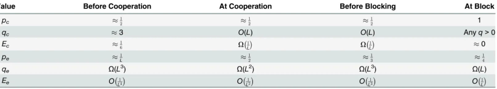
These numbers are derived for the most favorable target set (one that includes every assem-bly in any assemassem-bly sequence whose supremum is a valid terminal assemassem-bly that displays the property of the target set, defined as a perfectly placed blue signal that is generated when both red and green signals are present) and the most noncongruent partial assembly to produce it, as illustrated in Figs5and6. Likewise, the other counts can be estimated as shown inTable 1. This example demonstrates that, as to these target patterns,Gcdoes make a more efficient assembler than the noncooperative one. In general, cooperativity is a way to control the nega-tive effects of nondeterminism on efficiency. In fact, since misbinding of the cooperanega-tive C tile is the major cause of impurity, even partial experimental achievement of cooperativity is better than none.
Table 1. Efficiency of a cooperative assembler at temperatureτ= 2 and its noncooperative implementation at temperatureτ= 1.The substantial
drop in the probability of assembly with respect to the target set and its efficiency show the lack of robustness of the original assembler. Nevertheless, the data shows that some cooperation is better than none for efficiency of the assembler.
Value Before Cooperation At Cooperation Before Blocking At Block
pc
1
2
1
2
1
2 1
qc 3 O(L) O(L) Anyq>0
Ec 16 O
1
L O
1
L 0
pe 1L 12
1
3
1 4
qe Ω(L3) Ω(L2) Ω(L3) Ω(L)
Ee O L14
O 1 L2
O 1 L3
O1 L
Fig 5. The RGB assembler running in (noncooperative) experimental conditions can produce a variety of error patterns, both before and after the designed point of cooperation.Either the red, green,
or blue signal may set the radius (the size of the pattern.) Here, both signals attempt to fake cooperation by nondeterministically attaching a cooperation tile and spawning erroneous color signals. Each possible red and green signal may do so, producing a large quantity of error patterns.
doi:10.1371/journal.pone.0137982.g005
Fig 6. Past the point of cooperation, these phantom signals may or may not block one another, compounding the rate of error patterns.
By contrast to the previous two examples, our third example shows that strong assembly with perfect efficiency can be achieved at temperatureτ= 1, but on patterns that do not require
cooperation. An example is Meunier’s construction [17] by noncooperative assemblers for pro-ducing relatively large sets of 1D patterns for a given bound on the size (number of tile types) of the assembler. This construction shows that these assemblers are capable of assembling rea-sonably complex infinite families of terminal assemblies, where the complexity of the target pattern is measured by its size relative to the cardinality of the tile set. This holistic metric of complexity, however, does not address the issues of how strongly or efficiently the target set of patterns is being assembled. In [17], the author provides tree grammars for noncooperative tile assembly systems in the 2D planar aTAM. We begin our analysis by determining the target set P. In this case, the most naturalPis the set of terminal assemblies producible by some assem-bler such that each pattern in the target set has a height of5ðnþ2Þ
4 23, according to [17]. Since onlyfinite terminal patterns are desired, the target set should also contain promising patterns for the desiredfinite terminal patterns, as in the previous examples. A small example from [17] illustrates the point with a single-seeded assembler with 38 tile types. Meunier gives the size, measured by the 1D Manhattan diameter, as at most 27, so thatAn=Pn=Fare empty for n>27. Assembly proceeds from the seed, with tileable sites being occupied in a
nondetermin-istic order by tiles that bind stably with the existing aggregate. By design, it avoids costly nonde-terministic bindings which may produce nonpromising patterns or lead to infinite assembly sequences, a potential pitfall in noncooperative systems. Thus, as in the cooperative system, the assembler probabilistically assembles the target set with probabilityp= 1 (all target patterns are produced, and each assembled pattern is exactly some target pattern of the same size.) The impurity is equally easy to derive because it produces only target or promising patterns, there-fore the difference set of“junk”patterns is empty and perfect purity and efficiency are attained again. This is partially supported by the clever use of what Meunier calls“caves.”These geo-metric blocking artifacts constrain the assembly space by forcing new tiles to belong to either the construction of a cave, or the exploration of some previously constructed cave. Eventually, new cave construction ceases and all previously constructed caves are completely explored by the assembler. This halts the system’s growth. Similar to the frame in the RGB example above, the primary advantage of this geometric blocking relates to the impurity of the assembler. By ensuring that the assembler eventually exhausts its assembly space (an example of self-limiting assembly), the assembler avoids a largeq, which is apparent whenAisfinite. This analysis demonstrates that nontrivial target sets are probabilistically assemblable with perfect purity (anyq>0 will do) and arbitrarily large efficiencyEby noncooperative assembly systems in the
aTAM.
and the corresponding promising patterns leading to it forn<n0, as before, with all otherPn=
Fforn>n0. We can use the counts of nontarget patterns used in the calculation of his fidelity
to estimateqbased onn=n0since successful formation of the target pattern implies successful
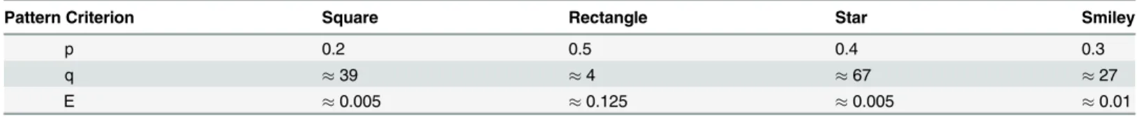
formation of smaller partial assemblies leading to it. The strengthpis grossly estimated from patterns that are least similar to the target by roughly counting the missing staples. For DNA origami, thep’s andq’s are shown inTable 2. Better estimates can be obtained from other ori-gami assemblers supported by gel electrophoresis as in [38]. Gels give a good indication of the
“junk”obtained at sizesn<n0. The protocol assembles origami squares into“superorigami”
structures with a reported yield of at least 95%. Our probabilistic analysis of this origami assembler yields values ofpcloser to 1 andqcloser to 0 using supplementary figures S8 and S9 from [38] including AFM images depicting folded squares with high congruency and gel elec-trophoresis showing little partially folded product or“junk”.
In each of the last three examples, the growth of the assembler is self-limiting or under severe assembly restrictions. Physically or metaphorically, these assemblers work inside of a finite assembly space as though on a prepared substrate or in a finite test tube. Meunier’s non-cooperative assemblers build walls as they grow the pattern, creating and then exploring finite caves in a process that eventually exhausts all possible future construction. The RGB assembler grows in a tiling space bounded by a given seed. Rothemund’s origami acts on a single finite strand (rather than the tiling notion of tile types in unbounded number.) In these systems, each new tile or staple constrains the space of possible future attachments, which allows for high efficiency. In the absence of these provisos, pumpable paths of tiles can yield extremely inefficient assemblers.
These examples show that the two concepts of assembly strength and assembly purity of an assembler with respect to a target set can vary independently, except for the case ofp= 1. Whenp= 1, the assembler must assemble all target patterns of every size, every assembled pat-tern must be a target patpat-tern, and there is no room for impurity. However, whenp<1,
assem-bled patterns may largely resemble target patterns but they still may be either target or junk patterns. A final family of examples described in detail in Appendix A exhibitdeterministic assemblers that assemble patterns with high probability close to but strictly smaller than 1 and still with perfect purity, for the set of target patterns assembled bynondeterministicand more complex assemblers with perfect strength and purity. These examples also illustrate how proba-bilistic assembly suggests a more general concept of simulation of an assembler by another that does not involved direct simulation of the dynamic process or kinetics of the original system. Because of the technical concepts involved, these systems are fully described in Appendix A.
General Results on Probabilistic Analysis
This section presents some general results that give a sense of the nature of probabilistic analy-sis, as well as its capabilities. One of the primary questions alluded to above is the relationship of the observable strengthpand impurityqto the probability of a pattern being assembled,i.e.,
Table 2. Strength and efficiency of DNA Origami assemblers.Values are roughly estimated based on their Monte Carlo sampling of the assembled prod-ucts, withpbeing estimated as the smallest fraction of well-formed subpatterns in the target pattern andqbeing estimated as the complement of his fidelity (fraction of correct origamis.) Due to incomplete information, these estimates disagree with the general perception that origami protocols are efficient assemblers.
Pattern Criterion Square Rectangle Star Smiley
p 0.2 0.5 0.4 0.3
q 39 4 67 27
E 0.005 0.125 0.005 0.01
the worst-case for the ratiospn=jAn\Pnj/jAnj, which is much harder to observe in an experi-mental setting or for very complex assemblers.
Theorem 1
If a set of patternsPis probabilistically assemblable with probability p, impurity q and effi-ciency E¼p
qby a monotonic pattern assemblerG, then
(a). target patterns are assembled with positive probability at leastpKpþq¼ KE
1þE>0,where K is the minimum positive probability of attachment of any single tile in the assembler; promis-ing patterns are assembled with positive probability at leastpþpq¼
E
1þE>0;
(b). nontarget (erroneous + nontarget promising) patterns are assemblable with probability at
most1 Kp
pþq¼
ð1 KÞpþq
pþq ¼
1þð1 KÞE
1þE .
(c). With respect to all assemblies, erroneous patterns are assembled with a complementary
probability to that of promising patterns and within the interval 0; 1
1þE
h i
.
Proof. Letpn,a0
n, andendenote the probabilities of target patterns, promising patterns, and
errone-ous patterns of sizenbeing assembled, respectively. For every sizen, the probability of a target pattern being assembled is given bypn:¼
jAn\Pnj
jAnj . The hypotheses thus guarantee that
jAn\Pnj
jPnj p, so thatpn¼
jAn\Pnj
jAnj ¼
jAn\Pnj
jPnj
jPnj
jAnjp
jPnj
jAnj, and that
en¼1 a
0
n¼
jAn A0nj
jAnj ¼ 1 jA0nj
jAnjq
jPnj
jAnj,i.e.,
1 a0
nq
jPnj
jAnjq pn
p pn
p
jA0nj
jAnj¼ q pa
0
nbecausepn
jA0nj
jAnj¼a
0
nsinceAn\PnA
0
n. Solving fora
0
nwe obtain thata
0
n
1
1þq
p¼ p
pþq>0,i.e., the
inequality in (a) holds for promising patterns. Now, since the assembler is monotonic, every target patternxis obtained from a nontarget promising patternain one step (as the last in a chain of only promising patterns), and then the probability ofxis given by the conditional probability
pðxÞ ¼pðxjaÞpðaÞ K p pþq;
whereKis the minimum probability of attachment of a single tile (here of the tile added toato obtainx.) Therefore, the inequality in (a) holds for target patterns as well. Statement (c) is straightforward from (a) and the fact that1 E
1þE¼
1
1þE. For inequality (b), The nontarget
pat-terns areEn[ ðA
0
n ðAn\PnÞ ¼An ðAn\PnÞ. Therefore,
enþa
0
n pn¼
jAn ðAn\PnÞj
jAnj ¼
jAnj jAn\Pnj
jAnj ¼
1 jAn\Pnj
jAnj
1 K p
pþq¼
1þð1 KÞE
1þE :
In manufacturing, the yield refers to the fraction of error-free target, in our notation jAn\Pnj/jAnj= (KE)/(E+1), while in chemistry it is described as the fraction of target product obtained of the theoretical optimum.
Another important question concerns information about the dynamic behavior of an arbi-trary assembler based solely on estimates of its strength and efficiency. The next results shows that a taxonomy of assemblers is indeed possible based on these parameters alone.
Theorem 2
If a set of patternsPis efficiently probabilistically assemblable by a pattern assemblerG, then one of the following three alternatives must hold:
(b). or the rate at which (erroneous + nontarget promising) are assembled switches in value in an alternating fashion;
(c). or the rate at which (erroneous + nontarget promising) are assembled is at least exponen-tial,i.e. |Ank| =O(α
nk)orjA0
nkj ¼Oðb
nkÞfor infinitely many n
k,for some constant rateα> 1 or some constant rateβ>1.
The proof requires the following concepts in real analysis in ordinary Euclidean space. A limit point of a given a sequence of real numbers {an}nis the limit of some converging subse-quence {anj}. Thus a converging sequence has only one limit point (its limit), but
nonconver-gent sequences such as {(−1)n} can have more than one limit point (such as ±1.) The well
known Bolzano-Weierstrass Theorem says that a bounded sequence of points in a real closed interval always has at least one limit point. This nonempty set of limit points for a sequence {an}nwill be denotedLim({an}).
Proof.
Letρnandνndenote the infinite sequences defined byrn:¼
jA0nj
jAnjandnn
:¼jAn A0nj
jAnj for the
corresponding sets of assembly for promising and erroneous patterns, as defined above. From Theorem 2(c), there follows that0r
nþnn<1 Kp
pþqfor every pattern sizen0, so these
sequences are bounded, andLim(ρn) andLim(νn) are nonempty sets, by the
Bolzano-Weier-strass Theorem.
IfLim(ρn) andLim(νn) consist of single elements, clearly condition (a) holds. Otherwise, letρ
andνbe the respective supremum (the smallest upper bound) of their nonempty limit sets. Only
one of two alternatives hold, eitherρ=νorρ6¼ν. Ifρ=ν, there must exist infinitely many cases
in whichρnνnholds and infinitely many cases in whichρnνnholds. Therefore there will be infinitely many intervals during which each of them predominates over the other, as stated in (b).
Otherwise,ρ6¼νand one type of patterns (promising or faulty) eventually dominates.
Given a promising or faulty patternxof sizen, let thecontextof an assembled pattern refer to a site where one tile may stably attach according to the given assembler and let theboundarybe the set of all contexts for an assembly of sizen. Ifxis faulty, every possible extension of the pat-tern will remain faulty, regardless of the boundary. Letαn(x) be the number of all such possible attachments. Ifxis promising, only a certain number of attachmentsβn(x) are not erroneous. The number of erroneous and promising attachments are complementary to the set of all pos-sible attachments. Letαnandβnbe the minimum ofαn(x) andβn(x) over all patternsxof sizen and letαandβbe the infimum (greatest lower bound) of allαn>0 andβn>0 over alln>0. Sinceρ6¼ν, at least one of them must be positive and, in fact, greater than 1 for infinitely many
n. Thereforeρncαnorνncβnfor infinitely manyn.
Discussion and Conclusions
assembler. A solution to the problem will likewise provide a way to compare the relative effi-ciency of two assemblers and a concept of the best assembler for the target set among a group of alternatives. A fairly general definition of probabilistic pattern assembly has been presented, along with an appropriate definition of efficiency of an assembler. The conditions require, not only that the assembler uniformly produce a certain fixed fractionpof the target patterns for every sizen, but that it have a good“idea”of the target set,i.e., that every assembled pattern of sizenshare a fractionpof some target pattern of the same size. The assembler is defined to have impurityqif it uniformly produces at most a factorqof nonpromising (junk) patterns for every sizenwith respect to the size of target patterns. The corresponding probabilistic analyses of typical assemblers in the self-assembly literature show that cooperative aTAM assemblers (at temperatureτ= 2) produce families of patterns deterministically with probabilityp= 1 and
arbitrarily large efficiency (with arbitrarily smallq>0), primarily because they only assemble
finite sets or unique patterns. Their efficiency, however, is substantially reduced when com-pared to the same assemblers run noncooperatively (at temperatureτ= 1),i.e., they are not
likely to be very robust assemblers experimentally. When assembling certain classes of infinite sets of 1D target patterns, nondeterministic assemblers can also perform at probabilityp= 1 and with arbitrarily large efficiency.
Examples also show that this concept of probabilistic assembly is valid and useful to com-pare the performance of different assembly systems on the same set of target patterns. Even if an ideal deterministic and cooperative assemblers is efficient, the corresponding assembler in which nondeterministic and noncooperative bonds are possible may, in general, be not effi-cient. Nevertheless, achieving any level of cooperation improves the efficiency over none at all. This result reinforces models like the kTAM [21], and motivates a search for mechanisms of cooperativity that are more experimentally accessible. When noncooperative assembly is appropriate or when cooperativity is not required, efficient assemblers are possible, and in fact, noncooperative assemblers inherently achieve them. Thus, because they are more likely to pro-duce good experimental results, applications that do not require cooperativity are worth exploring in detail in a search for more efficient assemblers. Probabilistic analysis produces results that are consistent with current intuition in algorithmic assembly models, while also providing some insights into the experimental feasibility of existing models.
Some general results have been established as well. First, every assembler assembling a target with strengthpand (im)purityqmust uniformly produce every target pattern with probability at least E
Eþ1, and erroneous patterns at a rate bounded by
KE
1þE, whereE¼
p
qis the efficiency of the
assembler andKis the minimum positive probability of attachment of a tile in the assembler. This framework and its results are quite general and apply to arbitrary assemblers, including the aTAM and experimental systems, as long as the system is monotonic,i.e., the assembly pro-cess can only enlarge the size of an assembly. The general results also demonstrate the utility of the model to examine or reason about efficiency or simulation of self-assembly without recourse to the details of the assembly model under consideration.
A number of questions are suggested by this probabilistic type of analysis of pattern forma-tion. First, the standard measure of complexity of an aTAM assembler has been the size of the tile set used to produce the target set. The efficiency is measured by the size of the assembled patterns relative to the size of the tile set. The notion of efficiencyEseems to bear no relation to the size of the tile set in the assembler. Is there any relationship between the two concepts? For example, it appears plausible that an upper and/or lower bound could be placed on the size of an optimal tile set necessary to simulate an assembler of a given strengthpand efficiencyE¼p
q.
producing the minimum amount of junk patterns. A larger efficiency indicates better strength and/or more purity (a smaller fraction of junk with respect to the set of target patterns.) By Theorem 1, efficiency ofE>1 guarantees that the probability of producing a promising
pat-tern is at leastK/2, as can be readily verified. IsE= 1 the appropriate threshold of efficiency that characterizes practical assemblers useful in the laboratory from assemblers that are not? Or, should one replacepandqby analogous functions of sizenand rather require that the ratiopn
qngrow at some polynomial ratef(jPnj) in the number of target patternsjPnj? Regardless
of the value, the related problem of then characterizing efficiently probabilistically assembl-able sets of patterns according to an appropriate threshold appears to be an interesting and difficult problem.
Third, the efficiencyEthus provides a way to holistically compare two assemblers of a target set for quality and, therefore, implicitly provides a criterion for choosing a best assembler for a given target set, namely one with unbeatable efficiency. How does this concept of optimality relate to the size of the most efficient tile set that assembles the given set probabilistically? At first glance, there appears to be no connection even for strict assembly (p= 1 and perfect effi-ciency), but one cannot completely rule out that a thrifty tile set may need to produce some junk to assemble the target patterns.
A fourth question posed by this approach is the exact power of nondeterministic assembly with respect to locally deterministic assembly. The examples show that running a cooperative assembler at temperatureτ= 1 substantially decreases its efficiency due to“errors”in the
coop-erative assembly that increase the nondeterministic choices in the assembly process. These examples show that there is a difference, but others in Appendix A also show that in some cases one might be able to“determinize”the assembly at the price of a smaller strength. Char-acterizing probabilistically determinizable assemblers is analogous to the corresponding com-plexity question and also appears to be a difficult problem.
Appendix
An important question in self-assembly is the power that nondeterministic assembly affords relative to deterministic models. Some insight into this question can now be obtained through probabilistic analysis because it allows a new way to compare the assembly power of different assemblers without resorting to direct dynamic simulation. The two examples below compare a particular kind of nondeterministic assembly system, namely probabilistic assemblers, to deterministic counterparts.
The assemblers are tile assembly implementations of cellular automata (CA). A CA is a computational model of a physical system defined on a homogeneous lattice, such as integer lattices in Euclidean spaces, by a set of rules that specify the state transitions of a discrete computational element at every node. Starting from a given seed as in the aTAM, a typical node/processorisynchronously updates its state to a valueδ(xi−1,xi,xi+1), according to a
com-mon local ruleδbased on the current state values of its immediate neighborsi−1,i(itself) and
the heightnof the pattern,i.e., the time it has taken the ECA to produce its assembly from the initial seed by the deterministic ruleδ.
There is a deterministic cooperative (temperatureτ= 2) tile assembler associated with every
ECA defined as follows.
1. Create one tile out of every 3 × 3 chunk of CA space time representing the transitionsa0i¼ dðai 1;ai;aiþ1Þanda00i ¼dða0i 1;ai0;a0iþ1Þ;
2. Label edges (with dashes) and corners (with dark quarter circles) whenever the value at that location is 1 (active);
3. ai−1,ai,ai+1are located at the W, NW and N locations, respectively, at timet(top line);
4. The valuea0i¼dðai 1;ai;aiþ1Þand possible flanking sites (4 values for 4 tiles)
ða0i 1;a0i;ai0þ1Þare located at W, C and E, respectively, at timet+1 (middle line); ifa0i¼1, then W and E are labeled;
5. a00i ¼dða0i 1;a0i;a0iþ1Þis located at the SE location at timet+2 (bottom line)
6. Create a new binding domain for each 3 bit binary number“read”from the edge of each tile
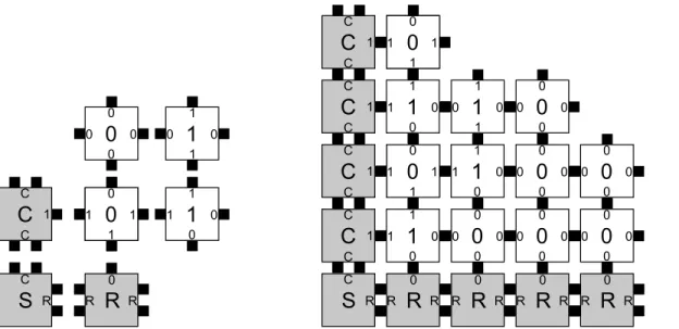
In the pattern of its glue types and symbols assigned to tiles, this tile set (Fig 7)(Left) assem-bles with probabilityp= 1 the target set of finite space-time 2D patterns generated by the origi-nal 1D ECA, on a given seed of arbitrary size. This tile set simulates the origiorigi-nal ECA in the following sense.
Definition 6.An assemblerGprobabilistically simulates assemblerHifGprobabilistically assemblesA(H),the set of patterns produced byH,with some probability p>0.GsimulatesH
ifGprobabilistically simulatesHwith p = 1.
A second example is the Domany-Kinzel Cellular Automaton (DKCA)[41], a 2D probabilis-tic assembler defined by a CA on binary states of radiusr= 1 whose transitions occur nondeter-ministically with probabilities given by
p½1j0;0 ¼0; p1¼p½1j0;1 ¼p½1j1;0; p2¼p½1j1;1
where 0/1 indicates an inactive/active (zero/nonzero) site andp[0j,] = 1−p[1j,]. Starting
from a given initial conditionsx0at timen= 0, simultaneous application of the transition rules defined byδwith the given probabilities produces another configurationxtat timet= 1, and iteration over time produces again 2D binary patterns of unbounded size by a random pro-cess. The DKCA is an abstract model of directed percolation, a phenomenon exhibited by directed spreading processes [41]. An important result in directed percolation theory is the existence of a phase transition from inactive (state 0) to active (state 1) global states as the com-bination ofp1andp2across a certain critical value on their way to 1, at which point the 2D
pat-tern generated is surely guaranteed to be percolating,i.e. locations in the seed are connected by paths of active sites to sites in the last row. An example of a percolating configuration is shown inFig 8(a) and 8(b)and the full active region is shown in the phase diagram on the right. We denote withPPercG the set of percolating patterns generated by a CA assemblerG.
A tiling system can again be designed that reproduces the space-time history of the DKCA, when operating at temperatureτ= 2. In the mapping from DKCA to assembly systems (Fig 7),
aggregate corresponds to the DKCA parametersp1andp2. For the weak assembly [35] of the
entire space-time history, there exists a concentration functionχwhich describes the relative concentrations of each tile to other tiles. With this mapping below, these tile assembly systems are parametrized by the DKCA parametersp1andp2as well.
It is straightforward to verify that these constructions guarantee that the two assemblers (the DKCA and the ECA tile sets) simulate each other with probabilityp= 1, according to Defi-nition 6. The assembler is maximally nondeterministic since, as usual, all tiles are available in saturation amounts. This observation implies the following result.
Theorem 3
The set of target patternsPDKCA(p1,p2)is strongly probabilistically assemblable with probability
p = 1 and perfect efficiency by the corresponding tile set described above for an arbitrary DKCA (p1,p2).
To address the question above, we are particularly interested in a target set of patterns assembled by this DKCA(p1,p2) tile set as an example to test whether certain nondeterministic
pattern assemblers can be found probabilistically equivalent todeterministicassemblers and if so, what exactly is the tradeoff involved in strength and efficiency, as defined in 5. This is in fact the case for several DKCA tile assemblers described next. The height of the pattern (corre-sponding to the time taken to generate it) is used as the appropriate notion of size.
Theorem 4
The target set of percolating configurationsPPerc
DKCAðp1;p2Þassembled by certain percolating DKCA(p1,p2)can be probabilistically assembled by a deterministic ECA tile assembly system
with high probability, but cannot be probabilistically assembled with probability p = 1.
Fig 7. Seed tiles and transition probabilities of probabilistic cellular automaton DKCA assemblers (Left).The tile set (Center) for ECA rule 122 uses
tile concentrations and nondeterminism to weakly assemble a variety of patterns (without spontaneous generation) from random seeds, as illustrated on the Right.
doi:10.1371/journal.pone.0137982.g007
Fig 8. DKCA patterns generated from the same seed can be wildly different (Left/Center).The DKCA phase diagram (Right) describes the observable behavior of the DKCA across a spectrum of probabilitiesp1andp2, with typical non/percolating behavior of an ECA assembler (shown as filled/empty circles,
respectively) consistent with the phase-transition DKCA behavior overall (the thresholding curve separates percolating from nonpercolating CA regions.)
Proof. We consider only ECA without the spontaneous generation of active sites (labeled 1), i.e., cells in the CA will remain inactive if the left and right neighbors are inactive, or, equiva-lently, such a cell will become active with probability 0 as a probabilistic CA. For a given DKCA(p1,p2), the target set of percolating patternsPpercDKCAðp1;p2Þincludes a wide variety of cluster shapes and sizes. From the construction of the assemblers, an ECA assembler essentially repro-duces the tiling coding of the space-time from any seed and therefore only prorepro-duces one pat-tern of a given height. In order to simulate a DKCA assembler, the transition rules of an ECA assembler have to be applied with the same probabilities (p1,p2). These probabilities arenot
identical to the probabilities in the transition rules of the ECA because its space-time generally has a structure that may eventually bias the applicable rules as the pattern is generated. How-ever, they can be empirically estimated from simulationsin silicoof the ECA from random ini-tial conditions. These restrictions, coupled with the fact that each seed only produces one pattern of a given size (height)n, imply that an ECA assembler can, in general, only reproduce a fraction of the set of percolating patterns generated by a DKCA at best. The ECA considered do not blanket the phase space evenly, as shown by simulation resultsin silicoon the Right in
Fig 8. However, for certain particular empirical valuesp1andp2, the ECA can probabilistically
assemble the set of percolating patterns produced by the DKCA(p1,p2) with a high probability
(p>0.9 in our simulations), as described next. Stochasticity in the tiling comes from the
ran-dom initial conditions.
The strengthpof the simulation was estimated experimentally as follows. For each candi-date ECA, 100 tiling simulations at size 300 were performed. Each tiling was run to completion (filling the simulation space as defined by the seed) at temperatureτ= 2 with no chance of
error or vacancy. Likewise, the corresponding DKCA for the empirical probabilities (p1,p2)
were simulated. By counting the actual use of each rule in the space-time history of the ECA over many runs and then determining the number of active children and inactive children gen-erated by the appropriate rules, an estimate can be given of which DKCA is producing the pat-terns. The space-times of the two assemblers were tested for percolation and thus how likely the two assemblers agree on the percolation property. Percolation in a finite assembly was determined by the presence of a spanning cluster of active sites that is incident on both the seed and the output row. An ECA assembler simulates the DKCA when it produces a set of pat-ternsAthat probabilistically assembles the targetPpercwith one of two thresholds,p>0.9 and
p>0.94. The resulting phase space diagram for the tile set reproduced the original DKCA
phase space diagram [41] at the sample points, as shown on the Right in (Fig 8). This shows that the ECA assembler generates a nonzero fraction of the DKCA patterns, and that it does not produce all of themi.e.,p<1.
Thus, these examples exhibit deterministic assemblers (ECA) that assemble patterns with high probability close to but strictly smaller than 1 and still with perfect purity, for the set of target patterns assembled by nondeterministic and more complex assemblers (DKCA) with perfect strength and purity. They also illustrate how probabilistic assembly suggests a more general concept of simulation of an assembler by another that does not involve direct simula-tion of the dynamic process or kinetics of the original system.
Acknowledgments
content and presentation of this paper. Simulations were supported by the University of Mem-phis High Performance Computing Center.
Author Contributions
Conceived and designed the experiments: TM MG RD. Performed the experiments: TM. Ana-lyzed the data: TM MG RD. Contributed reagents/materials/analysis tools: TM MG RD. Wrote the paper: TM MG RD.
References
1. Winfree E, Liu F, Wenzler LA, Seeman NC. Design and self-assembly of two-dimensional DNA crys-tals. Nature. 1998; 394(6693):539–544. doi:10.1038/28998PMID:9707114
2. Park SY, Lytton-Jean AK, Lee B, Weigand S, Schatz GC, Mirkin CA. DNA-programmable nanoparticle crystallization. Nature. 2008; 451(7178):553–556. doi:10.1038/nature06508PMID:18235497
3. Yurke B, Turberfield AJ, Mills AP, Simmel FC, Neumann JL. A DNA-fuelled molecular machine made of
DNA. Nature. 2000; 406(6796):605–608. doi:10.1038/35020524PMID:10949296
4. Zhang DY, Turberfield AJ, Yurke B, Winfree E. Engineering entropy-driven reactions and networks cat-alyzed by DNA. Science. 2007; 318(5853):1121–1125. doi:10.1126/science.1148532PMID: 18006742
5. Pei R, Matamoros E, Liu M, Stefanovic D, Stojanovic MN. Training a molecular automaton to play a game. Nature nanotechnology. 2010; 5(11):773–777. doi:10.1038/nnano.2010.194PMID:20972436
6. Maune HT, Han Sp, Barish RD, Bockrath M, Goddard WA III, Rothemund PW, et al. Self-assembly of carbon nanotubes into two-dimensional geometries using DNA origami templates. Nature nanotechnol-ogy. 2010; 5(1):61–66. doi:10.1038/nnano.2009.311PMID:19898497
7. Douglas SM, Dietz H, Liedl T, Högberg B, Graf F, Shih WM. Self-assembly of DNA into nanoscale three-dimensional shapes. Nature. 2009; 459(7245):414–418. doi:10.1038/nature08016PMID: 19458720
8. Tikhomirov G, Hoogland S, Lee P, Fischer A, Sargent EH, Kelley SO. DNA-based programming of quantum dot valency, self-assembly and luminescence. Nature nanotechnology. 2011; 6(8):485–490. doi:10.1038/nnano.2011.100PMID:21743454
9. Liedl T, Högberg B, Tytell J, Ingber DE, Shih WM. Self-assembly of three-dimensional prestressed ten-segrity structures from DNA. Nature nanotechnology. 2010; 5(7):520–524. doi:10.1038/nnano.2010. 107PMID:20562873
10. Qian L, Winfree E, Bruck J. Neural network computation with DNA strand displacement cascades. Nature. 2011; 475(7356):368–372. doi:10.1038/nature10262PMID:21776082
11. Zhao Z, Liu Y, Yan H. Organizing DNA origami tiles into larger structures using preformed scaffold frames. Nano letters. 2011; 11(7):2997–3002. doi:10.1021/nl201603aPMID:21682348
12. Hu H, Gopinadhan M, Osuji CO. Directed self-assembly of block copolymers: a tutorial review of
strate-gies for enabling nanotechnology with soft matter. Soft matter. 2014; 10(22):3867–3889. doi:10.1039/ c3sm52607kPMID:24740355
13. Zhang Z, Glotzer SC. Self-assembly of patchy particles. Nano Letters. 2004; 4(8):1407–1413. doi:10. 1021/nl0493500
14. Chandran H, Gopalkrishnan N, Reif J. Tile complexity of linear assemblies. SIAM Journal on Comput-ing. 2012; 41(4):1051–1073. doi:10.1137/110822487
15. Cook M, Fu Y, Schweller R. Temperature 1 self-assembly: deterministic assembly in 3D and probabilis-tic assembly in 2D. In: Proceedings of the twenty-second annual ACM-SIAM symposium on Discrete Algorithms. SIAM; 2011. p. 570–589.
16. Valiant LG. A theory of the learnable. Communications of the ACM. 1984; 27(11):1134–1142. doi:10. 1145/1968.1972
17. Meunier PÉ. Noncooperative algorithms in self-assembly. arXiv preprint arXiv:14066889. 2014;.
18. Rothemund PW, Winfree E. The program-size complexity of self-assembled squares. In: Proceedings of the thirty-second annual ACM symposium on Theory of computing. ACM; 2000. p. 459–468.