www.geosci-model-dev.net/5/975/2012/ doi:10.5194/gmd-5-975-2012
© Author(s) 2012. CC Attribution 3.0 License.
Geoscientific
Model Development
Analyzing numerics of bulk microphysics schemes in community
models: warm rain processes
I. Sednev and S. Menon
Dept. of Atmospheric Sciences, Lawrence Berkeley National Laboratory, Berkeley, CA, USA
Correspondence to:I. Sednev ([email protected])
Received: 14 May 2011 – Published in Geosci. Model Dev. Discuss.: 24 June 2011 Revised: 29 June 2012 – Accepted: 10 July 2012 – Published: 3 August 2012
Abstract. Implementation of bulk cloud microphysics (BLK) parameterizations in atmospheric models of different scales has gained momentum in the last two decades. Uti-lization of these parameterizations in cloud-resolving models when timesteps used for the host model integration are a few seconds or less is justified from the point of view of cloud physics. However, mechanistic extrapolation of the applica-bility of BLK schemes to the regional or global scales and the utilization of timesteps of hundreds up to thousands of seconds affect both physics and numerics.
We focus on the mathematical aspects of BLK schemes, such as stability and positive-definiteness. We provide a strict mathematical definition for the problem of warm rain for-mation. We also derive a general analytical condition (SM-criterion) that remains valid regardless of parameterizations for warm rain processes in an explicit Eulerian time inte-gration framework used to advanced finite-difference equa-tions, which govern warm rain formation processes in mi-crophysics packages in the Community Atmosphere Model and the Weather Research and Forecasting model. The SM-criterion allows for the existence of a unique positive-definite stable mass-conserving numerical solution, imposes an addi-tional constraint on the timestep permitted due to the micro-physics (like the Courant-Friedrichs-Lewy condition for the advection equation), and prohibits use of any additional as-sumptions not included in the strict mathematical definition of the problem under consideration.
By analyzing the numerics of warm rain processes in source codes of BLK schemes implemented in community models we provide general guidelines regarding the appro-priate choice of time steps in these models.
1 Introduction
and non-positive-definite time integration scheme could in-fluence the global water cycle causing artificial precipitation patterns that are then used as surface boundary conditions for ocean, land, lake, and sea ice models.
In the Weather Research and Forecasting (WRF) model version 3 (Skamarock et al., 2008), both the single mo-ment BLK schemes and the Morrison-Curry-Khvorostyanov double-moment BLK scheme (Morrison et al., 2005) (MCK05) might share similar deficiencies of non-positive and unstable solutions for warm rain processes if the mi-crophysical time step used is greater than a few tens of sec-onds. This feature of BLK schemes implemented in commu-nity models (CAM and WRF) could lead to possible erro-neous conclusions regarding the role of cloud microphysics and their influence on radiation or dynamics (amongst oth-ers) when relatively long time steps are used for integration. To avoid the uncertain performance of BLK microphysics schemes, if relatively long time steps are used for model integration and to improve the creditability of precipita-tion amount calculaprecipita-tions, we derive the necessary condi-tion (referred to as SM-criterion) to keep an explicit Eule-rian time integration scheme stable and positive-definite re-gardless of the parameterizations used for warm rain pro-cesses in BLK schemes. The SM-criterion constitutes the ex-istence of a unique positive-definite stable numerical solution and imposes constraints on the time step permitted (like the Courant-Friedrichs-Lewy condition for the advection equa-tion). We highlight that in addition to the limitations on the time step imposed by the dynamics, there also exists a limi-tation due to the microphysics. We also define well-behaved, conditionally well-behaved, and non-well-behaved Explicit Eulerian Bulk Microphysics Code (EEBMPC) classes and show that source codes of BLK schemes, which were origi-nally developed for use in cloud-resolving models and imple-mented in community models, belong to conditionally well-behaved EEBMPC class. We also provide recommendations regarding integration time steps for prospective simulations with WRF and CAM.
The paper is organized as follows. The general consid-erations are given in Sect. 2. The growth rate calculation due to warm rain processes in BLK schemes are discussed in Sect. 3. The comprehensive multi-step analysis of nu-merics for the system of differential equations that governs processes of warm rain formation in BLK scheme is pre-sented in Sect. 4. The first step in our analysis is the deriva-tion of a mass-conserving positive-definite analytical solu-tion for the linearized differential-difference equasolu-tions, pre-sented in Sect. 4.1. The second step in our analysis is the derivation of a numerically explicit Eulerian solution for the finite-difference equations, outlined in Sect. 4.2. The third step in the comprehensive analysis is the stability analysis for the numerical explicit Eulerian solution, given in Sect. 4.3. In Sect. 4.4 we show how the utilization of the “mass con-servation” technique might cause the violation of the sta-bility and positive-definiteness conditions when analytical
representation of autoconversion and accretion growth rates are known, using one of the BLK schemes as example. Dis-cussion and recommendations are provided in Sect. 5.
2 General consideration
We consider the following system of equations for bounded positive X(t ) and Y (t ) with initial conditions X(t=0)=
X0>0 andY (t=0)=Y0≥0 on time interval 0≤t≤τ:
dX
dt = −F (X)−G(X, Y ) , (1) dY
dt = +F (X)+G(X, Y ) , (2) whereF (X)andG(X, Y )are both positive and bounded, and positiveτ is given.
We are looking for a numerical solution forX(n+1)and Y (n+1)with initial conditions X(n)=X0 andY (n)=Y0
such that at each time step “n” satisfies the conservation equation
d[X+Y]
dt =0 (3)
as well as positiveness and boundedness conditions
0≤X(n+1)≤X0, (4)
Y0≤Y (n+1)≤X0+Y0, (5)
whereX(n)andY (n)areXandY at the beginning of time step “n”.
Explicit finite-difference scheme with time stepτis writ-ten as
X(n+1)=X(n)−τ[F (X(n))+G(X(n), Y (n))] (6) Y (n+1)=Y (n)+τ[F (X(n))+G(X(n), Y (n))]. (7) It is clearly seen that this solution conserves the sum ofX andY. By adding expressions (6)–(7) we get finite-difference analog for the conservation equation given by Eq. (3): X(n+1)+Y (n+1)=X(n)+Y (n).
The values ofX(n+1)andY (n+1)at the next time step are always bounded and positive only if
τmax≤
X(n)
3 Warm rain processes in community models
Applying these general considerations to cloud physics and defining
X=Qc>0
Y =Qr>0
F (X)=PAUTO>0 G(X, Y )=PACCR>0,
we obtain the following system of equations that governs the process of “warm” rain formation in prognostic BLK schemes:
∂Qc
∂t = −(PAUTO+PACCR) (9) ∂Qr
∂t = +(PAUTO+PACCR) (10) whereQcis cloud water mixing ratio,Qris rain water
mix-ing ratio, and PAUTO and PACCR are their changes due to auto-conversion and accretion, respectively. By adding Eqs. (9) and (10), we get
∂(Qc+Qr)
∂t =0. (11)
Equation (11) has the simple physical meaning. For the “warm” rain formation process total water mixing ratioQt=
Qc+Qrremains unchanged.
Different single-moment and double-moment BLK schemes used in CAM and WRF and referenced there-after as RaschCAM (Rasch and Kristjansson, 1998) and KESSLER (Kessler, 1969), LIN (Lin et al., 1983), ETA (Ferrier, 1994), TAO (Tao et al., 2003), THOMPSON (Thompson et al., 2004), MORRISON (Morrison et al., 2005), and WSM6 (Hong and Lim, 2006) schemes, respec-tively, calculate auto-conversion and accretion growth rates using a different non-linear analytical representation for functions PAUTO and PACCR. The system of non-linear differential Eqs. (9)–(10) is linearized and solved using an explicit Eulerian (EE) time integration scheme. Our analysis of source codes of MG08 scheme in CAM and TAO, THOMPSON, MORRISON, and WSM6 schemes in WRF, respectively, reveals that positiveness criterion (SM-criterion) similar to the inequality (8) and given by τmax≤
Qc
PAUTO+PACCR (12)
is never checked.
In our analysis of source codes for the BLK schemes re-ferred to above, we use the following definitions. Based on the validation of the SM-criterion we introduce definitions for three different classes that are a well-behaved EEBMPC class, a conditionally well-behaved EEBMPC class, and poorly-behaved EEBMPC class.
If the SM-criterion has always been validated and re-spected in EEBMPC, we define such a code as belonging to well-behaved EEBMPC class. The remarkable feature of a well-behaved EEBMPC is that it assures a unique sta-ble positive-definite mass-conserving numerical solution (re-ferred to as correct solution thereafter) for the governing dif-ferential equations. To the best of our knowledge, there is no well-behaved EEBMPC implemented in Community mod-els.
If the SM-criterion has never been checked in EEBMPC, we define such a code as belonging to a conditionally well-behaved EEBMPC class or a poorly-behaved EEBMPC class, whose common feature is that both rely on a so-called “mass conservation” technique in an attempt to avoid nega-tiveness of hydrometeors’ mixing ratios and make an explicit Eulerian time integration scheme positive-definite. As it is shown in the next section, the quintessence of the “mass con-servation” technique is an incorrect assumption: it assumes the existence of a positive numerical solution for the govern-ing differential equations in a time interval where this solu-tion is not defined.
The distinguishable feature of a conditionally well-behaved EEBMPC is that the SM-criterion is satisfied even if it has never been checked. As used in cloud resolving models or large eddy simulation models with temporal res-olution about a few seconds, conditionally well-behaved EEBMPC provides a correct solution for governing differ-ential equations because the limitation on the time step im-posed by dynamics is more restrictive than that imim-posed by microphysics (SM-criterion), and, in fact, the “mass conser-vation” technique is never applied. The transition between conditionally well-behaved EEBMPC and poorly-behaved EEBMPC is determined by the SM-criterion. If the time step used in a host model (CAM or WRF) is as those typically used for regional scale and especially large scale simula-tions and the SM-criterion is occasionally violated, a con-ditionally well-behaved EEBMPC would become a poorly-behaved EEBMPC. The eventual feature of a poorly-poorly-behaved EEBMPC is that it does not provide a correct solution for governing differential equations.
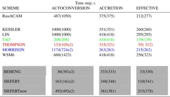
To avoid the use of an artificial “mass conservation” tech-nique, mimic the utilization of well-behaved EEBMPC, and provide guidelines regarding time steps permitted for model integration for prospective CAM and WRF users, we present maximal time steps for autoconversion and accretion pro-cesses as well as effective maximal time steps for both processes that are necessary to keep stability and positive-definiteness of an explicit Eulerian time integration scheme. These maximal time steps, which satisfy SM-criterion, are calculated for specified values of cloud water and rain water mixing ratios and two values of cloud droplet concentrations (Nc) for different BLK schemes and are shown in Table 1.
Table 1.Maximal time steps permitted to keep explicit Eulerian time integration scheme stable and positive-definite for autoconversion, accretion, and due to both processes in CAM and WRF bulk microphysics schemes. For comparison, the same values for Beheng (1994), Seifert and Beheng (2001), and Seifert and Beheng (2006) parameterizations are presented in gray. Maximal time steps shown forQc=
1.0 g kg−1,Qr=0.5 g kg−1,Nc=10(100)cm−3.
Time step, s
SCHEME AUTOCONVERSION ACCRETION EFFECTIVE
RaschCAM 487(1050) 375(375) 212(277)
KESSLER 1000(1000) 351(351) 260(260)
LIN 1000(1000) 418(418) 295(295)
TAO 208(208) 418(418) 139(139)
THOMPSON 133(105e2) 315(321) 93( 312)
MORRISON 1174(724e2) 263(263) 215(262)
WSM6 660(1423) 418(418) 256(323)
BEHENG 36(381e2) 333(333) 33(330)
SIEFERT 161(161e2) 348(348) 110(341)
SIEFERTnew 492(492e2) 381(381) 215(378)
cloud droplet concentrations (Nc) and indicate dependence
of autoconversion or accretion onNc=10(100) cm−3. For
example, the KESSLER scheme representation of both au-toconversion and accretion do not depend onNc, and for the
KESSLER row, values of time step are equal in each column. Non-dependence onNc, in the autoconversion column,
mani-fests non-applicability of KESSLER, LIN, and TAO schemes for cloud-aerosol interaction simulations, whereas, only the THOMPSON scheme accounts for dependence of accretion onNc. Except for this scheme, all other WRF BLK schemes
under consideration can be used for regional scale simula-tions if the time step in the host model does not exceed two to three hundred seconds. However, it should be noted that this conclusion is valid only for specificQc=1.0 g kg−1and
Qr=0.5 g kg−1 used to calculate maximal time steps
pre-sented in Table 1.
To demonstrate the instantaneous dependence of the effec-tive maximal time step on typical cloud water mixing ratio and rain water mixing ratio for different cloud types we de-fine a SM-number (Nsm) as
Nsm=
τ (PAUTO+PACCR) Qc
. (13)
It should be noted that there is an obvious relation-ship between the SM-criterion and the SM-number. The SM-criterion is valid (an explicit Eulerian finite-difference scheme is stable and positive-definite) if
Nsm≤1. (14)
Thus, the maximal time step permitted to keep an explicit Eulerian time integration scheme stable and positive-definite
corresponds to
Nsm=1. (15)
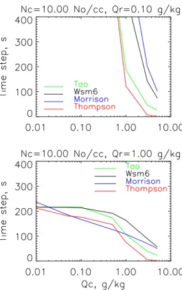
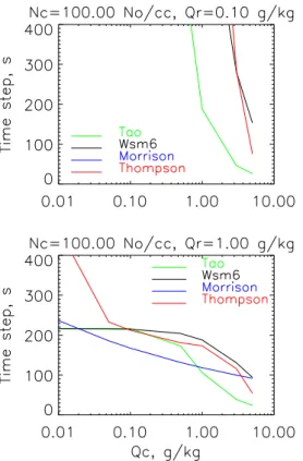
Maximal time steps calculated according to expres-sion (15) for TAO, THOMPSON, MORRISON, and WSM6 WRF BLK schemes as functions of Qc and Qr for two
different droplet concentration Nc=10 cm−3 and Nc=
100 cm−3, which are used as a proxy for clean “maritime” and “continental” clouds, are shown on Figs. 1 and 2 and Figs. 3 and 4, respectively. For “clean maritime” clouds, Fig. 1 shows instantaneous dependence of maximal time step on Qc for Qr=0.1 g kg−1 (top left), 0.5 g kg−1 (top
right), 1.0 g kg−1 (bottom left), and 3.0 g kg−1 (bottom right), respectively, whereas Fig. 2 shows instantaneous de-pendence of maximal time step on Qr for Qc=0.1 g kg−1
(top left), 0.5 g kg−1(top right), 1.0 g kg−1(bottom left), and 3.0 g kg−1(bottom right). Figures 3 and 4 replicate Figs. 1 and 2, respectively, for “clean continental” clouds.
Fig. 1.Maximal time step dependence onQcandQrforNc=10 cm−3.
Fig. 3.Maximal time step dependence onQcandQrforNc=100 cm−3.
step used in a multidimensional host model. For example, limitation on the time step provided in the WRF User Guide is given as
τwrf≤61Xwrf, (16)
whereτwrfis the time step in seconds and1Xwrfis the spatial
resolution in kilometers. However, this constraint does not account for additional restrictions due to the microphysics imposed by the SM-profiles that ensure an explicit Eulerian scheme stability and positive definiteness and reliability of model output. In fact, for regional or large scale WRF simu-lations with a time step chosen according to inequality (16) violation of the SM-criterion at different times, altitudes, and spatial locations leads to a non-positive-definite numerical solution for the governing warm rain differential equations.
To show that the SM-criterion is a necessary condition for an explicit Eulerian time integration scheme stability and positive-definiteness and to demonstrate the consequences of using the “mass conservation” technique, the next section de-scribes the multi-step analysis used.
4 Analytical and numerical solutions and stability analysis
Different single-moment and double-moment BLK schemes used in community models formulate auto-conversion PAUTO and accretion PACCR growth rates in a variety of ways providing different non-linear functional dependences on Qc, Qr, and Nc. The system of nonlinear differential
Eqs. (9)–(10) that governs the processes of warm rain forma-tion can be solved only numerically using iterative methods. However, if some linearization is assumed, they could also be solved analytically.
4.1 Warm rain processes: analytical solution
To solve the system (9)–(10) analytically, linearized on time interval 0≤t≤τ, both the auto-conversion growth rate PAUTO and accretion growth rate PACCR can be written as
AUTO=Cu0Q0c (17)
ACCR=Ca0Q0rQ0c (18)
where Q0c=Qc(t=0) >0, Q0r =Qr(t=0) >0, and Cu0
andCa0are given by
Cu0=PAUTO(Q0c)[Q0c]−1 (19) Ca0=PACCR(Q0c, Q0r)[Q0c]−1[Q0r]−1. (20) With expressions (17)–(20), Eqs. (9)–(10) are rewritten as follows
∂Qc
∂t = −AUTO−ACCR= −C
0 uQ
0 c−C
0 aQ
0 rQ
0
c (21)
∂Qr
∂t = +AUTO+ACCR= +C
0
uQ0c+Ca0Q0rQ0c. (22)
Solving forQcandQron time interval 0≤t≤τ we get an
analytical solution for linearized differential Eqs. (21)–(22): Qc=Q0c−t (Cu0+Ca0Q0r)Q0c (23)
Qr=Q0r+t (Cu0+Ca0Q0r)Q0c. (24)
It can be easily seen that solution (23)–(24) conserves mass. The analytical solution (23)–(24) is bounded and positive-definite if and only if
0≤Q0c−t (Cu0+Ca0Q0r)Q0c≤Q0c (25) Q0r ≤t (C0u+Ca0Q0r)Q0c+Q0r ≤Q0c+Q0r. (26) These inequalities determine the maximal time step permit-ted to keep a bounded and positive solution. Both are satisfied if the SM-criterion is valid:
t≤τmax=
1 C0
u+Ca0Q0r
. (27)
Thus, the SM-criterion determines the sufficient and neces-sary positiveness condition for the analytical solution to the system of differential Eqs. (21)–(22) regardless of the spe-cific formulations for autoconversion PAUTO and accretion PACCR growth rates. Condition (27) also determines the ap-plicability of the linearization given by expressions (17)– (20). At this point it should be clear that any assumption regarding the existence of the analytical solution for a time greater than that given by condition (27) is not sensible mathematically. The analytical solution for the linearized differential-difference Eqs. (21)–(22) permanently exists for any “t” on time interval 0≤t≤τmaxonly.
4.2 Warm rain processes: explicit Eulerian time inte-gration scheme
The finite-difference analog for the system of nonlinear dif-ferential Eqs. (9)–(10) that govern processes of warm rain formation can be given as
qcn+1−qcn
τ = −PAUTO−PACCR (28)
qrn+1−qrn
τ = +PAUTO+PACCR (29)
whereqcn andqcn+1,qrnandqrn+1are initial and new values of cloud water mixing ratio and rain mixing ratio, respec-tively. Time representations for auto-conversion and accre-tion growth rates are still not specified. In general, Eqs. (28)– (29) can be solved only using iterative numerical methods that need significant computational time. However, if some linearization is assumed, non-iterative computationally effi-cient numerical methods can be used. For example, in an ex-plicit Eulerian scheme a linearized exex-plicit form is used for both auto-conversion and accretion growth rates:
PAUTO=Cunqcn (30)
whereCunandCanare given by
Cun=PAUTO(qcn)[qcn]−1 (32) Can=PACCR(qcn, qrn)[qcn]−1[qrn]−1. (33) Explicit representation means that both auto-conversion and accretion growth rates can be calculated at the beginning of the microphysical time step becauseqcn andqrn are known. With expressions (30)–(33), Eqs. (28)–(29) are as follows:
qcn+1−qcn τ = −C
n
uqcn−Canqrnqcn (34)
qrn+1−qrn τ = +C
n
uqcn+Canqrnqcn. (35)
Solving forqc andqr we get a numerical solution for
lin-earized differential Eqs. (9)–(10):
qcn+1=qcn−τ (Cun+Canqrn)qcn (36) qrn+1=qrn+τ (Cun+Canqrn)qcn. (37) It is clearly seen that this solution conserves mass. By adding expressions (36)–(37) we get the finite-difference analog for the mass conservation equation given by Eq. (11):
qcn+1+qrn+1=qcn+qrn.
Despite the fact that the solution (36)–(37) conserves mass, it is not positive-definite. Whereasqrn+1 is always positive, qcn+1 sometimes might be negative. The numerical solution (36)–(37) is bounded and positive-definite if and only if 0≤qcn−τ (Cun+Canqrn)qcn≤qcn (38) qrn+1≤τ (Cun+Canqrn)qcn+qrn≤qcn+qrn. (39) These inequalities determine maximal time step permitted to keep a bounded and positive numerical solution. Both in-equalities are satisfied if the SM-criterion is valid:
τ≤τmax=
1 Cn
u+Canqrn
. (40)
Thus, the SM-criterion provides the necessary condition for the explicit Eulerian finite-difference scheme (34)–(35) to be positive-definite regardless of the parameterization formu-lae used for autoconversion and accretion growth rates (30)– (33).
An observation that the solution (23)–(24) for differential-difference equations and the solution (36)–(37) for finite-difference equations coincide is important, and its mathe-matical meaning is that the finite-difference scheme is sta-ble for fixed timesteps that do not exceed the maximal timestep given by the SM-criterion for the finite-difference equations (40). It should be clear that any attempt to solve the finite-difference Eqs. (34)–(35) using a timestep that is greater than that given by (40) is neither mathematically nor physically sensible because this situation is not governed by these equations in an explicit Eulerian time integration
framework. For a different time integration framework, the positive-definiteness condition and stability condition might differ. Stability is a very important issue that makes the finite-difference equations different from the differential-finite-difference equations for which the stability problem is not relevant. The analysis of stability is of crucial importance for any finite-difference scheme and should be done before its implemen-tation in a numerical model.
4.3 Stability analysis: explicit Eulerian scheme
The numerical solution (36)–(37) can be written as the matrix equation:
qcn+1 qrn+1
=
1−τ (Cun+Canqrn)0 τ (Cun+Canqrn) 1
×
qcn qrn
. (41)
The matrix characteristic equation for system (41) has the following form:
det
1−τ (Cun+Canqrn)−λ 0 τ (Cun+Canqrn) 1−λ
=0. (42)
For the finite-difference scheme to be stable it is necessary that all rootsλ1,2of its characteristic equation satisfy
|λ1,2| ≤1. (43)
However, in the case
−1≤λ1,2≤0, (44)
the numerical solution (36)–(37) might oscillate. This fact contradicts the conditions of positiveness (38)–(39). Thus, instead of inequality (43)λ1,2must satisfy
0≤λ1,2≤1. (45)
To find stability conditions for the scheme given by expres-sions (32)–(35) all the roots of the matrix characteristic equa-tion (42) have to be found. We then get the algebraic charac-teristic equation
λ2− [2−τ (Cun+Canqrn)]λ− [τ (Cun+Canqrn)+1] =0.(46) The solutions are as follows
λ1,2=
2−τ (Cun+Canqrn)±τ (Cun+Canqrn)
2 . (47)
The first rootλ1is given by
λ1=1, (48)
and stability inequality (45) forλ1is always satisfied.
The second rootλ2is given by
λ2=1−τ (Cun+Cnaqrn) . (49)
The right inequality is held unconditionally, but for the left inequality to be valid it is necessary that
τ≤τmax=
1 Cn
u+Canqcn
. (51)
The condition given by expression (51) is necessary for the computational stability of the finite-difference scheme given by expressions (32)–(35). Observation that conditions (40) and (51) coincide permits us to conclude that the SM-criterion provides the necessary condition for the explicit Eu-lerian finite-difference scheme given by Eqs. (34)–(35) to be stable and positive-definite regardless of the parameteriza-tion used for autoconversion and accreparameteriza-tion growth rates.
Because the stability of an explicit Eulerian time integra-tion scheme for microphysical governing equaintegra-tions used in BLK schemes has never been discussed, the effect of the vi-olation of the SM-criterion on its stability and positive defi-niteness is hidden. Since the validation of the SM-criterion is not reproduced in EEBMPCs used in community mod-els, these codes belong to the conditionally well-behaved EEBMPC class. Thus, we conclude that if relatively long time steps are used for WRF integration and the SM-criterion is occasionally violated, the source code implementations of the TAO, THOMPSON, MORRISON, and WSM6 schemes in the official WRF distribution would belong to poorly-behaved EEBMPC that do not provide a correct numerical solution for governing differential equations.
Although the source codes for these four schemes share the same deficiencies, in the following section we provide a detailed analysis of numerics of warm rain processes in conditionally well-behaved EEBMPC for the MORRISON scheme in WRF (Morrison et al., 2005) as well as Morrison-Gettelman scheme in CAM (Morrison and Morrison-Gettelman, 2008), because the numerical treatment of cloud water mixing ratio in both schemes is identical.
4.4 Warm rain processes in WRF: MCK05 numerical solution
The finite-difference analog for the system of differential equations for the double-moment BLK scheme is not pre-sented and discussed in Morrison et al. (2005).
In this scheme the warm rain formation processes are gov-erned by the system of differential equations (Khairoutdinov and Kogan, 2000) (KK2000):
∂qc
∂t = −c1[qc]
2.47[N
c]−1.79−c3[qc]1.15[qr]1.15 (52)
∂qr
∂t = +c1[qc]
2.47[N
c]−1.79+c3[qc]1.15[qr]1.15. (53)
Using “reverse engineering” (translating source code doc-umented in WRF to scientific notation used in the theory of finite-difference schemes), the finite-difference analog for
the system (52)–(53) can be written as qcn+1−qcn
τ = −q n
cc1[Ncn]−1.79[qcn]1.47−
qcnc3[qcn] 0.15[qn
r] 1.15
(54)
qrn+1−qrn τ = +q
n
cc1[Ncn]
−1.79[qn
c] 1.47+
qcnc3[qcn]0.15[qrn]1.15
(55)
where explicit representations for both PAUTO and PACCR are used:
PAUTO=qcnc1[Ncn]−1.79[qcn]1.47 (56)
PACCR=qcnc3[qcn]0.15[qrn]1.15. (57)
Explicit representation means that both the auto-conversion PAUTO and accretion PACCR growth rates, which are cal-culated at the beginning of the microphysical time step us-ing known qnc, qnr, and Nnc, are constants and can not be “ad-justed”.
Solving for qnc+1and qnr+1we get a numerical solution for the differential Eqs. (52)–(53):
qcn+1=qcn−
τ qcn{c1[Ncn]−1.79[qcn]1.47+c3[qcn]0.15[qrn]1.15}
(58) qrn+1=qrn+
τ qcn{c1[Ncn]
−1.79[qn
c] 1.47+c
3[qcn] 0.15[qn
r]
1.15} . (59)
It is clearly seen that this solution conserves mass. By adding expressions (58)–(59) we get a finite-difference analog for the mass conservation equation given by Eq. (11):
qcn+1+qrn+1=qcn+qrn.
Although the solution (58)–(59) conserves mass, it is not positive-definite, whereas qnr+1 is always positive, qnc+1
sometimes might be negative because the positiveness condi-tion given by the SM-criterion for the MORRISON scheme τ≤τmax=
1
{c1[Ncn]−1.79[qcn]1.47+c3[qcn]0.15[qrn]1.15}
,(60) whereτmaxis the time step permitted to keep positive
solu-tion, is not satisfied.
To avoid negative qnc+1, similar to the approach
usu-ally employed in other BLK schemes (e.g., Reisner et al., 1998) reduced artificial auto-conversion AAUTO and accre-tion AACCR rates are used (through the “mass conservaaccre-tion” technique):
AAUTO= q
n
cc1[Ncn]−1.79[qcn]1.47
τ{c1[Ncn]−1.79[qcn]1.47+c3[qcn]0.15[qrn]1.15}
(61)
AACCR= q
n
cc3[qcn]0.15[qrn]1.15
τ{c1[Ncn]−1.79[qcn]1.47+c3[qcn]0.15[qrn]1.15}
.(62)
original formulae (56)–(57) is clearly seen. Third, it is as-sumed that these expressions remain valid during timestepτ provided by a host model. However, as explained above, any attempt to use a timestep that is greater than that given by the SM-criterion (60) is not relevant in an explicit Eulerian time integration framework.
Because the SM-criterion is never checked in the EEBMPC for the MORRISON scheme, we classify this code as belonging to the conditionally well-behaved EEBMPC class. However, if the SM-criterion is violated for a particular “set” of{qc,qr,Nc, andτ}passed by a host model, the source
code for the MORRISON scheme would become poorly-behaved EEBMPC. An attempt to avoid negativeness of qnc+1
calculated according to the finite-difference Eq. (58) by ap-plying a “reduced” autoconversion AAUTO and accretion AACRR given by (61) and (62), respectively, that act during timestepτ > τmax(the “mass conservation” technique) is
ar-tificial and has nothing in common with the numerical solu-tion for the differential Eqs. (54)–(55) using the explicit Eu-lerian finite-difference Eqs. (58)–(59) that have no positive-definite and stable solution forτ > τmax.
If the SM-criterion is not respected, a poorly-behaved EEBMPC in the MORRISON scheme creates a virtual mi-crophysics reality characterized by a “virtual” cloud water mixing ratio (qncv) and rain water mixing ratio (qnrv) that are
used instead of a ”real” cloud water mixing ratio (qnc) and rain
water mixing ratio (qnr) supplied by the host model. These
virtual numbers can easily be calculated using the following procedure. If for input{qnc,qnr,Nnc, andτ}supplied by a host
model, Nsm>1, artificially “adjusted” AAUTO and AACRR
rates are calculated using formulae (61) and (62). Then a sys-tem of two equations for “virtual” qncvand qnrv derived by a) substitution of qncvand qnrvinstead of “real” qncand qnr, respec-tively, in Eqs. (56)–(57) and b) replacement of PAUTO and PACRR with AAUTO and AACRR in (56) and (57), respec-tively, has to be solved:
qcvnc1[Ncn]−1.79[qcvn]1.47=AAUTO (63)
qcvnc3[qcvn]0.15[qrvn]1.15 =AACCR. (64)
The remarkable feature of these “virtual” solutions qncv and
qnrv is that a “virtual” SM-number for the MORRISON
scheme (Nmv) defined as
Nmv=
τ{c1[Ncn]−1.79[qcvn]2.47+c3[qcvn]1.15[qrvn]1.15}
qn
c
(65) is always equal to one.
The mathematical meaning of the equality
Nmv=1 (66)
is that there is more than one available way to “adjust” orig-inal growth rates. The only condition is that a sum of artifi-cially “adjusted” positive virtual autoconversion VAUTO and accretion VACCR growth rates has to be equal to qnc/τ. Thus,
instead of the equality (66) a general definition for the “vir-tual” SM-number (Nsmv) that remains valid regardless of the
parameterization for autoconversion and accretion processes can be written as
Nsmv=
τ{VAUTO+VACCR}
qn
c
=1. (67)
However, even if a) virtual “adjusted” VAUTO and VACCR rates can be calculated by different methods (for example, for the MORRISON scheme these rates are given by AAUTO and AACCR, respectively) and b) their sum can exactly be equal to qnc/τ, there is no additional equation similar to (58)
that can be used for the calculation of qnc+1. As our analysis
in Sects. 4.1–4.3 shows, the finite-difference Eq. (58) is not valid for an arbitrary chosen timestepτ > τmax or,
equiva-lently, Nsm>1.
If Nsm>1, the expression (67) would constitute an
ad-ditional constraint that is not included in the strict mathe-matical definition of the problem introduced in Sect. 2. This expression is the general “mathematical foundation” of the “massConservation” technique, whose quintessence is an in-correct assumption: it assumes the existence of a positive-definite explicit Eulerian numerical solution in a time inter-val that is greater than that given by the general condition Nsm≤1, whereas our analysis shows that such a solution
does not exist in an interval whereτ > τmax.
The physical meaning of the general virtual SM-number (Nsmv) given by (67) is that “real” cloud water is
com-pletely depleted (qnc+1=0) by “adjusted” rates acting during
timestepτ (according to the finite-difference equation (58)), and it is thought, that the problem of negative cloud water mixing ratio on the next timestep is eliminated. The artificial growth rates, that use “virtual” qncvand qnrv(for example, for the MORRISON scheme these virtual numbers are given by the solution for the system (63)-(64)), are then passed to a host model for post-processing analysis.
this case, the output of a poorly-behaved EEBMPC contains artificially modified growth rates due to different microphys-ical processes.
5 Discussion
To date, there are no studies that analyzed the numer-ics of bulk microphysnumer-ics schemes with prognostic treat-ment of precipitating hydrometeors impletreat-mented in WRF (TAO, THOMPSON, MORRISON, and WSM6). Moreover, a finite-difference analog for each of these schemes has never been provided. Our analysis of source codes for these schemes in WRF reveals that a non-positive-definite explicit Eulerian time integration scheme is used to advance finite-difference microphysical equations.
Focusing on the mathematical aspects of BLK schemes, such as stability and positive-definiteness, we provide a strict mathematical definition for the problem of warm rain for-mation. We derive a general analytical condition (the SM-criterion) that remains valid regardless of parameterizations for autoconversion and accretion processes in an explicit Eu-lerian time integration framework used to advanced finite-difference equations that govern warm rain formation pro-cesses in BLK microphysics schemes. We also prove that the SM-criterion is a necessary condition of positive definiteness for the analytical solution of the linearized equations as well as a necessary condition of stability and positive-definiteness for an explicit Eulerian time integration scheme. The SM-criterion constitutes the existence of a unique positive-definite stable mass-conserving numerical solution, imposes an additional constraint on the timestep permitted due to the microphysics (like the Courant-Friedrichs-Lewy condi-tion for the adveccondi-tion equacondi-tion), and prohibits the use of any additional assumptions not included in the strict mathemati-cal definition of the problem under consideration. In general, preciseness of numerical scheme and time truncation errors would also be numerical issues to consider if there is a proof that a numerical scheme is stable and positive-definite.
Our analysis in Sects. 4.1–4.3 shows the non-existence of a unique positive-definite stable numerical solution in an explicit Eulerian time integration framework for differ-ential equations that govern warm rain microphysical pro-cesses for microphysical environmental conditions and an arbitrary chosen timestep for which Nsm>1. This
conclu-sion implies that any additional assumptions not included in the strict mathematical definition of the problem are not valid. One of these additional assumptions is the extrapola-tion of the existence of a positive-definite explicit Eulerian numerical solution to a time interval that is greater than that given by the general SM-criterion. The latter assumption is the quintessence of the so-called “massConservation” tech-nique that assumes that “adjusted” growth rates are appli-cable in a time interval where a positive-definite numerical solution does not exist. An understanding of the fact that the
numerical solution does not exist on an arbitrary chosen time interval is sufficient to reject the utilization of the “mass con-servation” technique, and any additional proof for its rejec-tion is not needed.
We highlight that the utilization of “mass conservation” technique applied to warm rain processes in an explicit Eu-lerian time integration framework is an incorrect attempt to avoid negativeness of cloud water mixing ratio. The “mass conservation” approach is conceptually incorrect because it relies on an assumption that “reduced” with respect to “orig-inal” autoconversion and accretion growth rates act during a given time step. This assumption contradicts a general rule used for the derivation of an explicit Eulerian finite-different representation for governing differential equations. In an ex-plicit Eulerian framework, the “original” growth rates are known constants calculated at the beginning of each micro-physical time step and can not be changed.
It is conventionally thought that the WRF model can be applied to a broad range of spatial scales from large eddy up to global scale simulations. However, for a prospective WRF simulation at a regional or global scale, the time step cho-sen according to recommendation provided in the user guide can cause occasional violations of the SM-criterion at dif-ferent times, altitudes, and spatial locations. An inappropri-ate choice of the time step leads to non-positive-definite nu-merical solution for the microphysical governing differential equations and degradation of the ability of WRF to calculate precipitation amount and its spatial and temporal distribu-tion. By introducing the concept of the SM-criterion vertical profile we provide a simple yet powerful tool that permits a rough estimation of an additional limitation imposed on the time step by microphysics and an appropriate choice for a time step for WRF simulations.
Depending on the validation of the SM-criterion in an EEBMPC, we introduce a definition for well-behaved EEBMPC, conditionally well-well-behaved EEBMPC, and poorly-behaved EEBMPC. In a well-behaved EEBMPC, the SM-criterion is always validated and satisfied, and a re-markable feature of well-behaved EEBMPC is an assur-ance of correctness of a numerical solution for the govern-ing differential equations. If the SM-criterion is never vali-dated, EEBMPC is assigned to a conditionally well-behaved EEBMPC class or poorly-behaved EEBMPC class, whose common feature is the utilization of the “mass conservation” technique.
Because the SM-criterion determines instantaneous tran-sition between conditionally well-behaved EEBMPC and poorly-behaved EEBMPC, the mechanistic extrapolation of applicability of conditionally well-behaved EEBMPC to re-gional (global) scales and the utilization for WRF integra-tion time steps on the order of hundreds (thousands) of sec-onds should be made with caution. As documented in the WRF user guide, limitation on time step permitted for model integration is imposed mainly by dynamics. However, this constraint does not account for additional restrictions due to microphysics imposed by the SM-criterion that ensures ex-plicit Eulerian time integration scheme stability and positive-definiteness. An occasional violation of the SM-criterion for this time step range determines the necessity of apply-ing the “mass conservation” technique to avoid negative-ness of cloud water mixing ratio that makes a conditionally well-behaved EEBMPC become a poorly-behaved EEBMPC (an explicit Eulerian time integration scheme becomes non-stable and non-positive-definite). The eventual feature of a poorly-behaved EEBMPC is that it does not provide a correct numerical solution for the governing differential equations.
Our analysis shows that the source code implementation of single moment (TAO, THOMPSON, and WSM6) schemes and a double-moment MORRISON scheme with a prog-nostic treatment of precipitating hydrometeors in WRF use the “mass conservation” technique and belong to the con-ditionally well-behaved EEBMPC class if used for cloud-resolving or large-eddy simulations, but they can become poorly-behaved EEBMPC for regional and large scale sim-ulations.
It should be noted that one of the most important aspects of numerical modeling is solving governing differential equa-tions using appropriate numerical methods. If governing dif-ferential equations are used, it is obvious that the milestones of applied mathematics, in general, and the theory of finite-difference schemes, in particular, should not be violated. The theory of finite-difference schemes is a branch of science that provides definitions for stability and positive-definiteness of finite-difference schemes (among many others). Our analy-sis of EEBMPCs in CAM and GFDL AM3 GCM reveals that these extremely important issues are not recognized as essential and crucial. For example, both CAM (Gettelman et al., 2008) and GFDL AM3 GCM (Salzmann et al., 2010) utilize diagnostic equations for precipitating hydrometeors, but the numerical treatment of cloud water remains similar to that used in EEBMPC with prognostic equations, which is discussed above. Additionally, both codes use a mechanistic approach, which is the utilization of equal time substeps be-cause long time steps are used for the host model integration. A feature of these codes is that at a minimum, two substeps are used even if stability and positiveness condition is oc-casionally satisfied. Moreover, even in a case having a few substeps, stability and positive-definiteness conditions (the SM-criterion) can be violated at different times, altitudes, and spatial locations.
Despite the fact that our analysis is focused on warm rain processes, we highlight that inclusion of the ice phase into consideration makes the SM-criterion even more restrictive because additional solid hydrometeors compete for the avail-able cloud water. For this case the SM-criterion is a necessary but not sufficient condition that should be included in any microphysics scheme whose numerics is based on an explicit Eulerian time integration framework.
As an alternative approach, numerical schemes different from an explicit Eulerian time integration analyzed in this pa-per can be used in BLK schemes. However, even if the gov-erning differential equations can be solved using stable and positive-definite finite-difference schemes, we would empha-size the need to re-evaluate the validity of the utilization of relatively long time steps in bulk microphysics schemes be-cause of the non-linear dependence of the growth rates of microphysical process on cloud characteristics. It is difficult to expect that the linearization of these growth rates remains valid for periods of time significantly longer than timesteps routinely used in cloud-resolving models. The computational expense of the utilization of smaller timesteps dictated by cloud physics considerations can be prohibitive. However, it is important to develop a numerical framework that is consis-tent from both the physics and numerics points of view and can be applied to any model regardless of scale.
Our future work is dedicated to the development of a pro-totype of a so-called open flexible microphysics interface. This interface consists of a suite of different stable positive-definite time integration schemes (explicit, implicit, and semi-implicit) and contains a process-oriented source code repository with libraries that include functions for calcula-tions of hydrometeor’s growth rates due to numerous micro-physical process routinely used in different BLK schemes. The distinguishable feature of the openFMI is its ability to “create new bulk microphysics schemes on the fly” elimi-nating necessity to support the multiple source codes for the BLK schemes in the host model.
Acknowledgements. The research at Lawrence Berkeley National Laboratory is supported by the US Department of Energy under Contract No. DE-AC02-05CH11231 This research was supported by the DOE Atmospheric System Research (ASR) program and Re-gional and Global Climate Modeling program. We also gratefully acknowledge support from Kiran Alapaty former program manager of the DOE ASR program. This research gratefully acknowledge resources provided by the National Energy Research Scientific Computing Center, under Contract No. DE-AC02-05CH11231.
References
Beheng, K. D.: A parameterization of warm cloud microphysical conversion processes, Atmos. Res., 33, 193–206, 1994. Collins, W. D., Rasch, P. J., Boville, B. A., Hack, J. J., McCaa, J. R.,
Williamson, D. L., Briegleb, B. P., Bitz, C. M., Lin, S.-J., and Zhang, M.: The formulation and atmospheric simulation of the Community Atmosphere Model version 3 (CAM3), J. Climate, 19, 2144–2161, 2006.
Ferrier, B. S.: A two-moment multiple-phase four class bulk ice scheme. Part I: Description, J. Atmos. Sci., 51, 249–280, 1994. Gettelman, A., Morrison, H., and Ghan, S.: A new two-moment
bulk stratiform cloud microphysics scheme in the Community Atmosphere Model, version 3 (CAM3). Part II: Single-column and global results, J. Climate, 21, 3642–3659, 2008.
Ghan, S. J. and Easter, R. C.: Computationally efficient approxi-mations to stratiform cloud microphysics parameterization, Mon. Wea. Rev., 120, 1572–1582, 1992.
Hong, S.-Y. and Lim, J.-O. J.: The WRF single-moment 6-class mi-crophysics scheme (WSM6), J. Korean Meteor. Soc., 42, 129– 151, 2006.
Kessler, E.: On the Distribution and Continuity of Water Substance in Atmospheric Circulations, Meteor. Monogr., No. 10, Amer. Meteor. Soc., Boston, 84 pp., 1969.
Khairoutdinov, M. and Kogan, Y.: A new cloud physics parameteri-zation in a large-eddy simulation model of marine stratocumulus, Mon. Wea. Rev., 128, 229–243, 2000.
Lin, Y.-L., Farley, R. D., and Orville, H. D.: Bulk parameterization of the snow field in a cloud model, J. Clim. Appl. Meteor., 22, 1065–1092, 1983.
Morrison, H. and Gettelman, A.: A new two-moment bulk strati-form cloud microphysics scheme in the Community Atmosphere Model, version 3 (CAM3). Part I: Description and numerical tests, J. Climate, 21, 3642–3659, 2008.
Morrison, H., Curry, J. A., and Khvorostyanov, V. I.: A new double moment microphysics scheme for application in cloud and cli-mate models. Part I: Description. J. Atmos. Sci., 62, 1665–1677, 2005.
Rasch, P. J. and Kristjansson, J. E.: A comparison of the CCM3 model climate using diagnosed and predicted condensate param-eterizations, J. Climate, 11, 1587–1614, 1998.
Reisner, R., Rasmussen, R. M., and Bruintjes, R. T.: Explicit fore-casting of supercooled liquid water in winter storms using the MM5 mesoscale model, Q. J. Roy. Meteor. Soc., 124, 1071– 1107, 1998.
Salzmann, M., Ming, Y., Golaz, J.-C., Ginoux, P. A., Morrison, H., Gettelman, A., Kr¨amer, M., and Donner, L. J.: Two-moment bulk stratiform cloud microphysics in the GFDL AM3 GCM: descrip-tion, evaluadescrip-tion, and sensitivity tests, Atmos. Chem. Phys., 10, 8037–8064, doi:10.5194/acp-10-8037-2010, 2010.
Seifert, A. and Beheng, K. D.: A double-moment parameterization for simulating autoconversion, accretion and selfcollection, At-mos. Res., 59–60, 265–281, 2001.
Seifert, A. and Beheng, K. D.: A two-moment cloud microphysics parameterization for mixed-phase clouds. Part I: Model descrip-tion, Meteorol. Atmos. Phys., 92, 67–82, 2006.
Skamarock, W. C., Klemp, J. B., Dudhia, J., Gill, D. O., Barker, D. M., Duda, M., Huang, X.-Y., Wang, W., and Pow-ers, J. G.: A Description of the Advanced Research WRF Ver-sion 3, NCAR Tech. Note, NCAR/TN-475+STR, NCAR, Boul-der, CO, USA, 125 pp., 2008.
Tao, W.-K., Simpson, J., Baker, D., Braun, S., Chou, M.-D., Fer-rier, B., Johnson, D., Khain, A., Lang, S., Lynn, B., Shie, C.-L., Starr, D., Sui, C.-H., Wang, Y., and Wetzel, P.: Microphysics, ra-diation and surface processes in the Goddard Cumulus Ensemble (GCE) model, Meteorol. Atmos. Phys., 82, 97–137, 2003. Thompson, G., Rasmussen, R. M., and Manning, K.: Explicit