SRef-ID: 1684-9981/nhess/2005-5-1 European Geosciences Union
© 2005 Author(s). This work is licensed under a Creative Commons License.
and Earth
System Sciences
Near-seismic effects in ULF fields and seismo-acoustic emission:
statistics and explanation
O. Molchanov1, A. Schekotov1, M. Solovieva1, E. Fedorov1, V. Gladyshev1, E. Gordeev2, V. Chebrov3, D. Saltykov3, V. I. Sinitsin3, K. Hattori4, and M. Hayakawa5
1Inst. of the Physics of the Earth, Russian Academy of Sciences, Bolshaya Gruzinskaya 10, 123995, Moscow D-242, Russia 2Inst. of Volcanology, Petropavlovsk-Kamchatski, Kamchatka, Russia
3Inst. of Geophysical Survey, Russian Academy of Sciences, Far-East Branch, Petropavlovsk-Kamchatski, Kamchatka, Russia
4Marine Biosystems Research Center, Chiba University, 1-33, Yayoi, Chiba 263-8522, Japan 5University of Electro-Communications, Chofu 1-5-1, Tokyo 182, Japan
Received: 20 July 2004 – Revised: 10 November 2004 – Accepted: 12 November 2004 – Published: 3 January 2005 Part of Special Issue “Precursory phenomena, seismic hazard evaluation and seismo-tectonic electromagnetic effects”
Abstract. Preseismic intensification of fracturing has been investigated from occurrence analysis of seismo-acoustic pulses (SA foreshocks) and ULF magnetic pulses (ULF fore-shocks) observed in Karimshino station in addition to seis-mic foreshocks. Such analysis is produced for about 40 rather strong and nearby isolated earthquakes during 2 years of recording. It is found that occurrence rate of SA fore-shocks increases in the interval (−12, 0 h) before main shock with 3-times exceeding of background level in the interval (−6, −3 h), and occurrence probability of SA foreshocks (pA∼75%) is higher than probability of seismic foreshocks (ps∼30%) in the same time interval.ULF foreshocks are masked by regular ULF activity at local morning and day-time, nevertheless we have discovered an essential ULF in-tensity increase in the interval (−3, +1 h) at the frequency range 0.05–0.3 Hz. Estimated occurrence probability of ULF foreshocks is about 40%. After theoretical consideration we conclude: 1) Taking into account the number rate of SA fore-shocks, their amplitude and frequency range, they emit due to opening of fractures with size ofL=70–200 m (M=1–2); 2) The electro-kinetic effect is the most promising mechanism of ULF foreshocks, but it is efficient only if two special con-ditions are fulfilled: a) origin of fractures near fluid-saturated places or liquid reservoirs (aquifers); b) appearance of open porosity or initiation of percolation instability; 3) Both SA and ULF magnetic field pulses are related to near-distant fractures (r<20–30 km); 4) Taking into account number rate and activation period of seismic, SA and ULF foreshocks, Correspondence to:O. Molchanov
it is rather probable that opening of fractures and rupture of fluid reservoirs occur in the large preparation area with hori-zontal size about 100–200 km.
1 Introduction
Fracturing is a basic process in the Earth’s lithosphere. Tradi-tional analysis of fracturing is registration of seismic pulses (shocks) at the ground surface. Famous Gutenberg-Richter law describes averaged occurrence rate of the fracturing. It states that number of opening fractures in the time unit (Nt=∂N/∂t) depends mainly on the magnitudeM or linear size of the fracture Land on level of the regional tectonic activityA; dependence onLshows distribution with fractal exponentc=2b+1, b∼0.9 (see discussion later). Thus, in the seismo-active area like Japan the large fractures (M=6-7,
L=10–50 km), usually treated as noticeable earthquakes, oc-cur several times per year while moderate fractures (M=3–4,
10 100 1000 Hypocentral Distance, km
3
Fig. 1. CurvesKs=Ks∗ = 1 (solid line) and Ks=0.1 (line with
closed circles) in coordinatesM (magnitude),R(hypocentral
dis-tance). They indicate limiting distancesR∗(M) for earthquakes
with defined value ofMand threshold of sensitivityKs∗. Each
indi-vidual EQ is represented by point in this plot. The criterionKs>Ks∗
means that EQ points above these curves are included into consid-eration. Limiting distances from observation of seismo-acoustic emission at Matsushiro station in Japan (Gorbatikov et al., 2002) are shown by curve with stars.
for large earthquakes (M>6–7), but its duration is several days or less for moderate earthquakes (M=4–5). Duration of foreshock series is shorter than aftershock one; b) Incom-plete sequence main shock- aftershocks when foreshock se-ries is absent and the earthquake looks as a sudden event. c) Ascending (foreshock) and descending (aftershock) series of moderate earthquakes without clear climax, so-called earth-quake swarm. It looks as incomplete sequence without large main shock while its usual duration is several weeks. Un-fortunately, the occurrence probability of the complete se-quence is not very high (20–30%; Scholz, 1990) and a ques-tion immediately arises whether an earthquake with sudden start is a regular phenomenon or the absence of foreshocks is due to lack of the seismometer sensitivity. The next ques-tion is an origin of the sequence itself. As concerns after-shocks, they are usually explained by residual relaxation of strain-stress increase generating a main shock. Inverse pro-cess of the stress accumulation and related dilatancy could be in principle responsible for appearance of foreshocks as it was discussed in numerous papers some times ago (see e.g. discussion in Scholz, 1990). However, it has been re-cently discovered that the value of stress increase or stress drop caused by an earthquake is not so large and dilatancy fracturing due to stress accumulation is negligible. It leads sometimes to conclusion that there is no preparatory (precur-sory) stage of an earthquake (Main, 1997). Obviously, this
Fig. 2. (a)SA pulses±12 days from 13 April 2002 EQ (M=4.9,
D=128 km, H=45 km, Ks=1.4). Upper panel: yellow stars are
time andKsvalue of 13 April 2002 EQ, and the weaker EQ which
happened 8 days before (Ks=0.5) together with variation of
atmo-sphere wind velocity. Lower panel: Amplitudes of SA pulses (in arbitrary units). There is some known correlation with atmosphere
wind but a connection with EQ-s is also seen. (b)SA and ULF
observational results in the vicinity (±24 h) of the earthquake 13
April 2002 (M=4.9,D=128 km,H=45 km,Ks=1.4) happened in
day-time (16:48 LT). Upper panel presents recording of seismome-ter: amplitude of the EQ shock (star) and weak foreshock about 4 h ahead. Next panel shows the intensity of ULF magnetic field vari-ations in the frequency band 0.003–0.1 Hz (NS and EW horizontal components). Third panel from above shows the intensity of pul-sating SA signal and last panel shows the wavelet spectrum of ULF horizontal component intensity.
Fig. 3.The same as in Fig. 2b but for EQ 15 March 2003 (M=6.4,
D=187 km,H=5 km, Ks=26.1, which happened at morning time
(06:12 LT).
small-size fracturing but lose a possibility to detect signals from far-distant areas (see Sect. 5). There are a lot of re-ports on wide-band SA emission before large earthquakes. For example Morgunov et al. (1991) recorded a distinctive anomaly in SA noise behavior in the rangeF=800–1200 Hz about 16 h before the famousM=7.0 Spitak earthquake, Ar-menia, 1988, at the distance 80 km from the epicenter. Gor-batikov et al. (2002) found an increase of the SA intensity av-eraged over 20 min in the frequency range fromF=25 Hz to
F=1000 Hz in a time 2–12 h before several moderate earth-quakes (M=4–5) at the Matsushiro station in Japan. They discovered that the frequency channel F=25–35 Hz is the most sensitive to seismisity. Unlike them, we are going to analyze pulsating component of SA signals (Sects. 3 and 4). Three types of ULF electromagnetic signals associated with earthquakes have been reported till now. The first (in time in-terval±several minutes around main shock) is a co-seismic signal (e.g. Eleman, 1965; Takeuchi et al., 1997), which ap-pears just after the shock and probably is initiated by strong seismic pulse induction (Surkov et al., 1999; Molchanov et al., 2001), it is hardly connected with preseismic fracturing. The second type is preseismic noise-like ULF magnetic field emission in the time interval several days or weeks before large earthquakes (Fraser-Smith et al., 1990; Haykawa et al., 1996; Kopytenko et al., 2002). However, a relation of this emission to preseismic fracturing is not proved. More-over, our observations in Karimshino showed a clear depres-sion of ULF magnetic field intensity several days before the earthquakes. The effect is probably connected with seismo-induced perturbations in the atmosphere-ionosphere and ev-idently has no relation to the foreshock activity (Molchanov et al., 2003). Therefore, we pay attention to the third type of ULF signals, so-called near-seismic ULF magnetic field pulses in the time interval several hours ahead of the main shock. A well-known case of such an event is so-called ULF magnetic emission 2–3 h before large Spitak earthquake (Molchanov et al., 1992; Kopytenko et al., 1993)
(a)
(b)
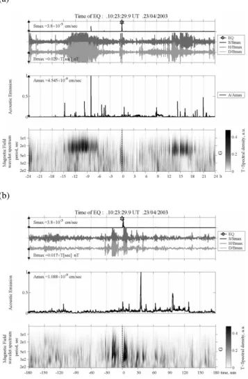
Fig. 4. (a)The same as in Fig. 2b but for EQ 23 April 2003 (M=5.8,
D=485 km, H=10 km, Ks=1.5), which happened at late evening
time (20:53 LT).(b)Extension of the (a) to the interval±3 h from
the seismic shock.
2 Equipment and seismic index
During 1999–2000, in addition to the existing seismic and geophysical observations, Russian and Japanese scien-tists established a special observatory at Karimshino site (52.94◦N, 158.25◦E) in Kamchatka (Far-Eastern Russia). Its main purpose is to study a correlation of seismic activity with electromagnetic and other nonseismic phenomena. The main advantage of this station is quiet electromagnetic envi-ronment that allows us to use rather sensitive equipment and to check some theoretical ideas. The regular recordings have been started since June 2000 and some information about Karimshino station is already published (Uyeda et al., 2002; Molchanov et al., 2003).
31 May 2002 6.1 842 1.1 10 91 6.09 0 > 10 10 day
8 Sept. 2002 5.5 379 1 53 -169 5.2 0 > 10 23 day HFULF 8 Oct. 2002 5 151 1.5 27 97 9.18 0 >5+noise 18 -
16 Oct. 2002 6 132 12.5 113 -175 10.12 0 0 + 1 20 Oct. 2002 5 150 1.5 29 89 1.34 0 2 4 day 18 Dec. 2002 5 113 2.2 42 82 11.09 0 > 5 15 -
1 Jan. 2003 4.9 145 1.2 29 92 1.33 1 20 > 5 20 day HF ULF 6 Feb. 2003 5.1 147 1 159 163 4.42 0 > 10 22 day
15 Mar. 2003 6.4 187 26.1 5 116 19.41 1 16 > 10 21 + 1 19 Mar. 2003 6.2 191 16.8 5 110 14.42 4 13 > 10 16 - 25 Mar. 2003 5.1 189 1.3 17 116 13.24 1 1 > 10 13 - 23 Apr. 2003 5.8 485 1.5 10 46 10.23 1 8 > 10 15 + 0.5 17 May 2003 5 181 1.1 16 135 1.46 1 6 >5 21 day 12 Aug. 2003 5.1 191 1.3 5 161 11.45 0 3 19 -
legend:
1. Date of selected strong and nearby earthquake (Ks≥ 1)
2. Magnitude of the earthquake. 3. Epicenter distance, km. 4. Ks index.
5. Hypocenter depth, km.
6. Azimuth calculated from the North direction clockwise 7. Universal time (LT= UT + 10h30m)
8. Number of seismic foreshocks during a day before the earthquake. 9. Time of the first seismic foreshock, hours before earthquake. 10. Number of SA foreshocks.
11. Time of the first SA foreshock, hours.
12. Presence of ULF foreshocks (+) or strong morning-day time ionosphere-magnetosphere emission (day) several hours before earthquake.
13. Time of the first ULF foreshock, hours.
14. Specific high-frequency (F=1-4 Hz) ULF spectrum changes before earthquake.
2001 in addition to wide-band SA receiver (accelerometer type) we have installed a resonant SA receiver, which is tuned near frequencyF=30 Hz. It has high sensitivity for pulsating seismo-acoustic signals (Saltykov et al., 1998).
Here we analyze ULF magnetic and SA data during 2 years of regular observations from 1 September 2000 to 1 October 2003. A parameter characterizing seismic influence is necessary for the correlation analysis of seismic and non-seismic data. The non-seismic characteristics, such as magnitude
M, epicenter distanceD, depthH, are presented in seismic catalogues. We assume that the index of seismic activity is proportional to seismic energy input1Es=∫P sdt∼<Ps>τ, where Ps is seismic energy flux and τ is duration of seis-mic pulse. Ps is decreasing with distance due to divergence
of flux in space (∼R−2), inelastic attenuation (coefficient
Fa) and scattering or elastic attenuation (Aki and Richards, 1980). Scattering can be described in terms of multi-ray propagation and in the first approximation the scattering fac-tor inPs is inversely proportional toτ. Hence:
1Es ∼=
Es/R2
Fa∼(101.5M/R2)Fa(R, M), (1) where Kanamori and Anderson (1975) scaling is used and
R=(D2+H2)1/2.
We introduce a seismic indexKsas following (Molchanov et al., 2003):
Ks= p
Fig. 5.Results of data analysis in the case of the EQ on 8 May 2002
(M=5.8,D=167 km,H=21 km,Ks=8.5, LT=14:42). Upper panel
is seismic recording, next panel is ULF intensity in the frequency
rangeF=1–4 Hz for all 3 components of the magnetic field
varia-tion, then it is SA signal amplitude, and at the last panel impedance
ratioZ/Gis shown for the same HF ULF frequency range as in the
second panel.
where8a=√Fa∼=(1+2R/La)−2.66. HereLais attenuation distance and it is easy to find thatLa∼=QL∼=2×10M/2(km), whereQ∼=100 is elastic quality andLis average size of the seismic source (Aki and Richards, 1980).
The dependencies for Ks=1 and Ks=0.1 in M, R co-ordinates are presented in Fig. 1. In such a presentation the lineR (M, Ks= constant) shows the limiting distance for a given threshold K∗
s= constant determined by mech-anisms of nonseismic effects and sensitivity of a receiver. Recently Gorbatikov et al. (2002) reported about the bursts of seismo-acoustic emission (SAE) registered at Matsushiro station (Japan) in association with rather large seismic shocks (M=3−5). They found that a separatrix occurs between earthquakes accompanied by SAE bursts and earthquakes without SAE bursts if the results are plotted in M-R diagram. The equation of the separatrix is written as follows
M=M(R∗)=1.77 logR∗+1.13. (3) This dependence is also depicted in Fig. 1. It is evident that the limiting distance enlarges whenKs decreases. Change ofKs-threshold from 1 to 0.1 leads approximately to 3-times distance enlargement and about(Ks∗)−1increase of reception area.
3 Case study
In order to exclude aftershock series and swarms we have selected only strong and nearby earthquakes (Ks≥1), with no strong preceding shocks (Ks>0.5) for at least 3 days. We have found 25 such earthquakes with magnitude from
M=4.5–6.5. Main parameters of the earthquakes are pre-sented in Table 1. Example of SA data in the time span of±12 days around 13 April 2002 EQ (M=4.9,D=128 km,
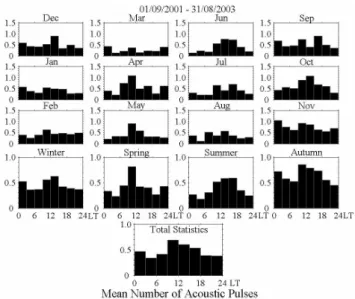
Fig. 6.Averaged number of SA pulses/(per 3 h)=NAin dependence on local time and for different seasons.
H=45 km,Ks=1.4, row 7 in Table 1) is shown in Fig. 2a to-gether with variation of atmosphere wind velocity, which is one of the main SA induction sources. SA and ULF observa-tional results in the interval±24 h from time of the shock are shown in Fig. 2. Both foreshock and aftershock series are ab-sent in seismometer recording in this case (except one weak foreshock 4 h ahead) but SA foreshock series do exist. As for ULF magnetic field signals, we can not find clear connec-tion with seismic shocks due to daily variaconnec-tion of ULF inten-sity related mainly to magnetic pulsations from ionosphere and magnetosphere. These magnetospheric signals appear usually at morning-day time (e.g. Ansari and Fraser, 1986; see also next section) and can mask the signals from under-ground. An other example is shown in Fig. 3. The same as before, foreshock series in seismometer recording are absent but the SA foreshocks are clearly seen. ULF response is also questionable here probably due to morning time of observa-tion. However, in the case presented in Fig. 4, in which seis-mic shock happened at evening time, some unusual pulses about 1 h before seismic shock can be supposed.
Note that unlike spectrum of morning-day time magnetic pulsations from ionosphere-magnetosphere with periods 20– 30 s (see Fig. 4a), the ULF signals suspected for associa-tion with earthquake have more wide-band spectrum, which stretches from periods 100–150 s to about 1s (Fig. 4b). It is interesting also that total duration of the ULF pulse is about 10 min and internal structure with shorter pulses of about 1 min duration can be seen.
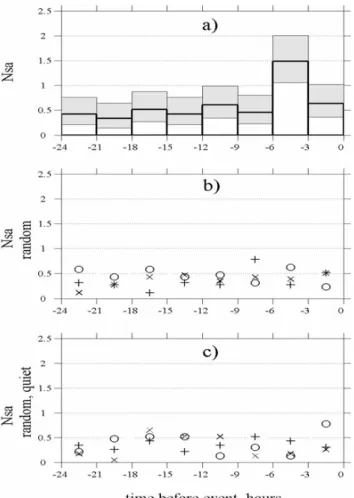
Fig. 7. (a)Upper panel: Seismic activity in terms ofKs values during 2 years of observation. Distribution of averaged number
of pulses during 1 day before strong seismic shocks (Ks≥0.5) for
seismic foreshocks (middle panel) and for SA foreshocks (panel be-low). Amplitude of the foreshock is proportional to size of the black circle. Aftershock influence is excluded by selection (see text). Dis-tribution averaged on 33 strong and nearby earthquakes is shown on
right. Background level ofNApulses is shown by dash line.
Molchanov et al., 2003). An example of the analysis is pre-sented in Fig. 5. While the result seems interesting, we have found that this type of analysis is not very reliable for revela-tion of pulsating ULF activity due to presence of atmospheric pulses from thunderstorms and man-made interferences inZ -component. Nevertheless we include these results in Table 1.
4 Statistics
Let us estimate the statistical properties of nonseismic fore-shocks. Taking into account that SA pulses can be generated not only by fracturing but also by atmosphere winds, tides, temperature and man-made sources (Gordeev et al., 1991; Saltykov et al., 1998) we find firstly overall average occur-rence rate of SA pulses. Diurnal and seasonal variations of the number of impulses with amplitudes higher than double averaged amplitudeNA are shown in Fig. 6. It can be seen that averagedNA≈0.5. Then we plot averagedNAin the in-terval (−24 h, 0) before selected seismic strong and nearby earthquakes (Ks≥0.5, 33 seismic events) in Fig. 7a. As be-fore (see description of Table 1 in the previous section), we exclude the aftershock influence. It is evident that in the in-terval (−6 h, −3 h) NA exceeds background level about 3 times and total interval of SA foreshock intensification is about 12 h before a seismic shock. In order to be sure that the result is reliable, we estimate the confidence intervals of the distribution and in addition the distribution of SA pulses for random selection of 33 event dates both in the interval of 2 years and in the interval of three months from 1 June 2002 to 31 August 2002, when earthquake activity is weak (see Fig. 7a). These estimates are presented in Fig. 7b. We think they demonstrate non-coincidental relation of SA foreshock intensification to selected strong and nearby seismic shocks.
Fig. 7. (b)Panel a): Averaged distribution of SA pulses 1 day before 33 strong and nearby seismic events (the same as on right of (a) but with indication of 98% confidence intervals by grey rectangulars up and down. Thick lines are mean values). Panel b): Mean number of SA pulses in eight 3 h intervals before events for 3 independent samples with random event time (33 events in each sample from 1 September 2001 to 31 August 2003). Panel c): Mean number of SA pulses in eight 3 h intervals before events for 3 independent samples with random event time for quiet interval (33 events in each sample, from 1 June 2002 to 31 August 2002).
In fact, our estimation is similar to known BSR (boot strap resembling) method, when the statistics is not robust as in our case.
Fig. 8. Averaged overall ULF magnetic field daily variation and spectrum.
over 3 days before the seismic shock. We conclude that a reliable intensification of ULF intensity (about 3 times above background variation) occurs in the time interval (−3 h, +1 h) whenKs≥1.
Now we estimate the occurrence probability of SA and ULF foreshocks. Number of background SA pulses in the interval 12–15 h before EQ is about 2–2.5 (see Figs. 6 and 7). Referring to Table 1, we can consider each case with number of SA foreshocks more than 5 as the case of frac-turing intensification. Because we have 19 such cases from 25, our estimation of SA foreshock occurrence probability is pA=76%. If we define the seismic foreshock series as occurrence of more than one pulse during one day before earthquake, then it can be seen from Table 1 that occurrence probability of seismic foreshocks is 20%, but if we take into account each foreshock event, then seismic foreshock proba-bility isps=44% (11 events from 25). Similar estimation of ULF foreshock probability is hampered by above-mentioned magnetic pulsation intensification in morning-day time. ULF probability during nighttime ispm=28%. However, if we take into account ULF foreshock findings in Table 1 both in amplitude variation in the frequency range F≤0.1 Hz and in HF ULF range (F=1–4 Hz), then ULF probability is
pm=44%.
5 Discussion
Our results demonstrate that absence of seismic foreshocks for earthquake with sudden inclusion does not mean absence of earthquake preparation stage. Thus, the existence of defi-nite precursory process is in compliance with not only com-mon sense but also with observational evidences.
We use the index Ks and corresponding limiting dis-tance of the preparation zone R(M, Ks)=R∗ (see Fig. 1) as characteristics of precursory process. It looks as deter-ministic assumption. However, it can be considered as a result of averaging on ensemble of more or less individ-ual earthquake events. Note that for Ks∼1, Rast∼La/2 (Lais the seismic attenuation distance,La=QL∼=2×10M/2, then observational relationship (Eq. 3) can be reduced to
R∗=0.23∗100.56M∼=0.23∗100.06MLa/2. It means that the size of preparation zone is approximately equal to the dis-tance of resultant distribution of seismic energy. The
spec-Fig. 9.Distribution of normalized ULF horizontal component
inten-sity in the frequency rangeF=0.05–0.3 Hz for different ensembles
of selected earthquake shocks with different thresholds and in the interval 12 h before and 2 h after each shock.
trum of seismic or SA pulse is the following (see e.g. Molchanov et al., 2002):
(∂u/∂t)ω=u0Cs p
τ/2π /(π r)x2(1+x2)−3/2exp(−xr/La),(4) where is final slip (≈10−4L),x=ωτ0,τ
0=L/(2Cr),Cs≈Cr are velocities of seismic wave and rupture. The spectrum depends on distance r and size L, Fig. 10, and for dis-tances r≪La the spectrum maximum is near x=√2 or F=Fm=√2Cr/(π L)≈1350/L(m) Hz.
It is obvious that, unlike conventional seismometer, the SA narrow-band receiver is sensitive to opening of small frac-tures with size from 20 to 200 m (valuesMfrom 0 to 2), the reception distances (or attenuation distances) for such frac-tures lie between 5 and 20 km.
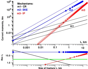
As for ULF foreshocks, we take into account three known models of electromagnetic field generation due to fractur-ing: the first is CR model, in which charge relaxation dur-ing fracture opendur-ing is considered (Gershenzon et al., 1989; Molchanov and Hayakawa, 1995); the second (EKE) model is based on mechanism of electro- kinetic conversion in a course of water diffusion just after crack opening in order to compensate changes in high pore pressure around crack (Mizutani et al., 1976; Jouniaux and Pozzi, 1995; Fenoglio et al., 1995) and the third is model of inductive electromagnetic pulses (IP) arising in a course of seismic wave propagation inside the conductive ground medium. This model was pro-posed by Surkov (1999) and also discussed by Molchanov et al. (2001) for explanation of co-seismic ULF magnetic and electric field variations. Estimations of the mechanisms ef-ficiency for rather realistic values of parameters in terms of the current moments are in Fig. 11.
2 3 5 2 3 5 2 3 5
0.1 1.0 10.0 100.0
Frequency, Hz
Fig. 10. Power spectrum of seismic shock in dependence on
frac-ture sizeL=2 km (M≈4), solid line andL=50 m (M≈1), line with
open circles (recording of deformation velocity) or line with closed circles (accelerometer). Both spectrums are at the distance of
seis-mic attenuation (r=La≈100L).
Let us consider now a possibility of noise-like SA or ULF fracturing emission. It depends on occurrence rate of frac-turing. Background number rate of seismic pulses in the range of magnitudes fromM∼7 to aboutM∼3 is described by Gutenberg-Richter relationship:
Nt(L∗ ≤L)=A(L∗)−2b. (5)
It means that number rate density is as follows:
∂Nt/∂L(L, L+dL)=2bA(L)−(2b+1). (6) Usually accepted value of constant b≈0.9. This value is keeping approximately during fracturing intensification. It was found (Evernden, 1986) from observation of many after-shock series thatb=0.7–1.2, therefore we suppose the same distribution in foreshock series but extend it for smallerL
values by simple assumption concerning size-volume den-sity:
∂2Nt/∂V ∂L=B(r)/Lc. (7)
Number density in the point of observationr0is the follow-ing:
∂Nt/∂L= Z
Vf
∂2Nt/∂V′∂Lexp(−R/La)dV′. (8)
where Vf is a region of fracturing intensification, R=r0−r′
and we assume for simplicity an exponen-tial model of limiting factor with R∗∼La=QL. In a case of far-distant activation region: R≫(Vf)1/3, ∂Nt/∂L=<B>Vfexp(−<R>/QL)/Lc. By comparing with Eq. (6) we find immediately that for L>R/Q,
<B>Vf=2bA and c=2b+1≈2.8. Note that assumption (Eq. 7) with c≈3 corresponds to so-called L−3 criterion,
Size of fracture L, km
Fig. 11. Above panel: estimation of current moments of different
ULF generation mechanisms in dependence of fracture sizeL, CR
model is solid line, EKE model is line with closed circles, IP model is line with triangles(see text for description of the models). Below: normalized reception distance for different models.
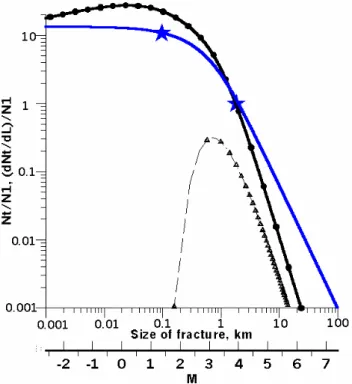
which was exploited in many papers on fracturing emission (e.g. Gershenzon et al., 1989). However, in a case of far-distance activation area we cannot expect any pulses from small-size fractures as it is shown in Fig. 12. Let us suppose now that the activation region is so large that includes near-distant sites andBdoes not depend on distance critically. In a case of flattened out cylinder with characteristic horizontal sizeD0∼100 km and vertical sizeH∼10 km, which is about depth of the crust, the approximated Eq. (8) can be re-written as follows
∂Nt/∂L≈<B>V0L3−c/ h
(L2+D20/Q2)(L+H /Q)i, (9) whereV0=π D20H. The result both for number rate density and cumulative number rate together with observational val-uesNtis also shown in Fig. 12.
For origin of noise-like signal we suppose a pulse overlap-ping or condition:
Ntτ≥1. (10)
It is true both for correlated and not correlated pulses. In our problem the duration of seismic pulse τ≈aτ0≈aL/(2Cr), where a is elongation of the pulse due to elastic scattering (a<Q). Had dependence (Eq. 5) be valid even for small-est values of L we could expect generation of emission from opening of small fracture (crack) ensemble with size
Fig. 12. Number rate density in the point of observation in a case of the far-distant region of fracturing (dash line with triangles) and in a case of large fracturing region including observation site
(hori-zontal dimensionD0=100 km, thicknessH=10 km; line with closed
circles). Cumulative number rate for latter case is solid line. All
the values are normalized toN1=Nt(L≥2 km)≈10−5s≈1/per day.
Observational values are shown by stars. It is evident that model of the large activation zone is more compatible with our observation results.
The situation is different for ULF pulses generated by the EKE mechanism. In this case, the duration of pulse
τm≈L2/(4Dw), whereDw≈(1–100) m2/s is the coefficient of water diffusion through porous ground medium (Mizu-tani et al., 1976; Fenoglio et al., 1995). Using the condi-tion (Eq. 10) for values Nt in Fig. 12 it can be seen that ifL≥50–100 m then ULF generation could be either noise-like (Dw∼1 m2/s) or pulsating (Dw∼100 m2/s). Note that large values ofDwcan be explained by percolation instabil-ity (Fenoglio et al., 1995; Jouniaux and Pozzi, 1995) and limiting distances of ULF foreshocks for the same scales as related to SA pulses (L=50–200 m) are 2.5–10 km (see Fig. 11).
We believe that our conclusions about the large area of fracturing activation before an earthquake and about the con-nection of the preparation process with unstable fluid dif-fusion are helpful for understanding the earthquake origin. Furthermore, the combined analysis of the fracturing inten-sification can be useful for earthquake forecast. For exam-ple, if we assume mild criterion of the forecast: one fore-shock signature from three possible ones (seismic, SA, ULF), then supposing above-mentioned valuesps≈30%,pa≈75%, pm≈40%, the forecast probability of EQ time is about 90%. But if we use more strict criterion : at least two type
fore-shocks from 3 possible ones, the forecast time probability is about 50%. Of course, the probability of false alarms should be taken into consideration. Therefore, a reliability of the EQ time and position forecast can be essentially improved if we develop the network of stations like Karimshino observatory.
Acknowledgements. Authors are thankful to S. Uyeda and P. F.
Bi-agi for helpful discussion of the results. This research is performed under ISTC grant 1121.
Edited by: P. F. Biagi Reviewed by: two referees
References
Aki, K. and Richards, P.G.: Quantitative seismology, W. H. Free-man and Comp., San Francisco, 1980.
Ansari, I. A. and Fraser, B. J.: A multistation study of low lati-tude Pc3 geomagnetic pulsations, Planet. Space Sci., 34, 519– 531, 1986.
Eleman, F.: The response of magnetic instruments to earthquake waves, J. Geomagn. Geoelectr., 18, 1, 43–72, 1965.
Evernden, J. F., Archambeau, C. B., and Cranswick, E.: An evalu-ation of seismic decoupling and underground nuclear test moni-toring using high-frequency seismic data, Rev. Geophys., 2, 143– 215, 1986.
Fraser-Smith, A. C., Bernardy, A., McGill, P. R., Ladd, M. E., Helli-well, R. A., and Villard Jr., O. G.: Low frequency magnetic field measurements near the epicenter of the Loma-Prieta earthquake, Geophys. Res. Lett., 17, 1465–1468, 1990.
Gershenzon, N. I., Gokhberg, M. B., Karakin, A. V., Petviashvili, N. V., and Rykunov, A. L.: Modelling the connection between earth-quake preparation process and crustal electromagnetic emission, Phys. Earth Planet Inter., 57, 129–138, 1989.
Gladyshev, V., Baransky, L., Schekotov, A., et al.: Some prelimi-nary results of seismo-electromagnetic research at Complex Geo-physical Observatory, Kamchatka, in: Seismo-Electromagnetics
(Lithosphere-Atmosphere-Ionosphere Coupling), edited by:
Hayakawa, M. and Molchanov, O., Terrapub, 2002.
Gorbatikov, A. V, Molchanov, O. A., Hayakawa , M., Uyeda, S., Hattori, K., Nagao, T., Nikolaev, A. V., and Maltsev, P.: Acoustic emission, microseismicity and ULF magnetic field per-turbation related to seismic shocks at Matsushiro station, in: Seismo-Electromagnetics (Lithosphere-Atmosphere-Ionosphere Coupling), edited by: Hayakawa, M. and Molchanov, O., Ter-rapub, 1–10, 2002.
Gordeev, E. I., Saltykov, V. A., Sinitsyn, V. I., and Chebrov, V. N.: Effect of Earth’s surface heating on high-frequency seismic noise, Dokl. Akad. Nauk SSSR, 316, 85–88, 1991.
Fenoglio, M. A., Johnston, M. J. S., and Byerlee, J. d.: Magnetic and electric fields associated with changes in high pore pressure in fault zone-application to the Loma Prieta ULF emissions, J. Geophys. Res. Solid Earth, 100, 12 951–12 958, 1995.
Jouniaux, L. and Pozzi, J. P.: Streaming potential and permeability of saturated sandstones under triaxial stress: Consequences for electrotelluric anomalies prior to EQs, J. Geophys. Res., 100, 10 197–10 209, 1995.
netic phenomena associated with earthquakes, Geophys. Res. Lett., 3, 365–368, 1976.
Mogi, K.: Earthquake Prediction, Academic Press, 355, 1985. Molchanov, O. A., Kopytenko, Yu. A., Voronov, P. M., Kopytenko,
E. A., Matiashvili, T. G., Fraser-Smith, A. C., and Bernardy, A.: Results of ULF magnetic field measurements near the epicenters of the Spitak (Ms=6.9) and Loma Prieta (Ms=7.1) earthquakes: comparative analysis, Geophys. Res. Lett., 19, 1495–1498, 1992. Molchanov, O. A. and Hayakawa, M.: Generation of ULF electro-magnetic emissions by microfracturing, Geophys. Res. Lett., 22, 3091–3094, 1995.
Molchanov, O. A.: Fracturing as an underlying mechanism of Seismo-Electric Signals, in: Atmospheric and Ionospheric Elec-tromagnetic Phenomena Associated with Earthquakes, edited by: Hayakawa, M., Terra Sci. Publ. Comp., 349–356, 1999.
bridge University Press, 439, 1990.
Surkov, V. V.: ULF electromagnetic perturbations resulting from the fracture and dilatancy in the earthquake preparation zone, At-mospheric and Ionospheric Phenomena Associated with Earth-quakes, edited by: Hayakawa, M., TERRAPUB, 357–370, 1999. Takeuchi, N., Chubachi, N., and Narita, K.: Observation of earth-quake waves by the vertical earth potential difference method, Phys. Earth Planet. Inter., 101, 157–161, 1997.
Uyeda, S., Nagao, T., Hattori, K. et al.: Japanese-Russian