65
© 2015 GEUS. Geological Survey of Denmark and Greenland Bulletin 33, 65–68. Open access: www.geus.dk/publications/bull
Observed melt-season snowpack evolution on the
Greenland ice sheet
Charalampos Charalampidis and Dirk van As
Due to recent warm and record-warm summers in
Green-land (Nghiem et al. 2012), the melt of the ice-sheet surface
and the subsequent runof are increasing (Shepherd et al.
2012). About 84% of the mass loss from the Greenland ice sheet between 2009 and 2012 resulted from increased sur-face runof (Enderlin et al. 2014). h e largest melt occurs in the ablation zone, the low marginal area of the ice sheet (Van As et al. 2014), where melt exceeds wintertime accumulation and bare ice is thus exposed during each melt season. In the higher regions of the ice sheet (i.e. the accumulation area), melt is limited and the snow cover persists throughout the year. It is in the vast latter area that models struggle to calcu-late certain mass l uxes with accuracy. A better understand-ing of processes such as meltwater percolation and refreezunderstand-ing in snow and i rn is crucial for more accurate Greenland
ice-sheet mass-budget estimates (Van Angelen et al. 2013).
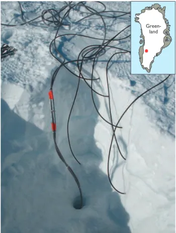
In May 2012, the i eld campaign ‘Snow Processes in the Lower Accumulation Zone’ was organised by the Geological Survey of Denmark and Greenland (GEUS) at the KAN_U automatic weather station (67°0´0˝N, 47°1´1˝W; 1840 m above sea level), which delivers data to the Programme for Monitoring of the Greenland Ice Sheet (PROMICE; Van As
et al. 2013) and is one of the few weather stations located in the lower accumulation area of Greenland (Fig. 1, inset). During the expedition, we installed thermistor strings, i rn compaction monitors and a snowpack analyser; we drilled i rn cores, performed i rn radar measurements, gathered me-teorological data, dug snow pits and performed dye-tracing experiments. One important objective of the campaign was to understand the thermal variability in the snowpack dur-ing the melt season by monitordur-ing with high-precision tem-perature probes (Campbell Scientii c temtem-perature probe, model 107; accuracy: better than ± 0.4°C over the range –24 to 48°C).
Six temperature probes were installed in the snowpack of the previous winter at depths of 0.05, 0.10, 0.20, 0.30, 0.40 and 0.70 m below the surface (Fig. 1). h e data from the probes were stored at 30-minute intervals on data loggers, which also triggered additional measurements of radiation-shielded air temperature at 1.10 m, surface albedo and surface-height change due to accumulation and ablation. Emitted longwave
radiation was also recorded to be able to calculate the surface
temperature assuming snow to be a black-body radiator. h e
vertical position of the probes relative to the surface, which changes due to ablation and accumulation, was determined by the sonic ranger measurements. Recorded temperatures at er the probes surfaced were discarded.
h e relatively shallow snowpack (0.70–0.80 m) was on
top of i rn of density ρ >500 kg m-3 which had
accumulat-ed in the previous years (Fig. 1). In the upper i rn we found ice lenses (ρ >800 kg m–3) several metres thick. Within the
snowpack, two thin ice layers were present, one at 0.30 m
Green-land
66 66
and one at c. 0.50 m below the surface, both about 0.01 m
thick. h e average density of the snow was determined to be
roughly 360 kg m–3, yielding an accumulation of 0.25 ± 0.08
m water equivalent (w.e.) since the summer 2011
(Charalam-pidis et al. 2015). Below, we present observations from the
period 02 May to 23 July and interpret the atmosphere–sur-face interaction and its impact on the subsuratmosphere–sur-face snow layers, with the goal to quantify refreezing in the Greenland accu-mulation area.
Atmosphere–snow interaction
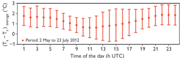
h e observations reveal a strong similarity between the
near-surface air temperature and the snow-near-surface temperature with changes of air temparature lagging on average 30–40 minutes behind. Typically, the air remained warmer than the snow surface (Fig. 2), implying a prevailing stable stratii ca-tion of the near-surface air. At night, the dif erence was larg-er (1.6–1.9°C) due to the reduced sunlight and subsequent cooling of the surface forced by longwave radiation. During the day, the temperature dif erence was smaller (0.6–1.2°C) primarily due to solar radiation heating the surface and re-ducing atmospheric stability. Understandably, when air temperature exceeds 0°C, the temperature dif erence can be larger since the surface cannot exceed the melting point.
On 6 May, overcast conditions and atmospheric stillness caused the increase of air temperature above +6°C (Fig. 3A).
h ese were the highest temperatures during the
observation-al period and similar temperatures occurred observation-also on two days in June (3 and 18). With the exception of 6 May, the air tem-perature remained negative until the last week of May. Dur-ing this period, the temperature of the upper 0.20 m of snow followed a pronounced diurnal cycle, which at 0.20 m lagged about 10 hours behind the variations in surface temperature (Fig. 3B), signifying the low thermal conductivity of snow.
At 1840 m above sea level, the ice sheet generally experi-ences low melt rates. When melt occurs, it displays a diurnal cycle following air temperature. A diurnal cycle of positive air temperatures occurred i rst on 27 May, marking the
be-ginning of the melt season (Fig. 3A). h e surface ablated in
response to the warm conditions, while the snow tempera-tures revealed the distinct progression of a warming and thus wetting front moving vertically through the snowpack (Fig.
3B). h e temperature at 0.70 m depth was af ected by this
42 hours at er surface melt initiated, i.e. an average warming front progression of only c. 17 mm h–1. h e entire snowpack
became temperate at er six days of ablation. h e slow
pro-gression of the warming front indicates a concurrent hetero-geneous meltwater ini ltration to the i rn below (Humphrey
et al. 2012).
During the period 8–12 June, sub-freezing air tempera-tures occurred again (Fig. 3A) and melting ceased. While the upper part of the snowpack remained close to 0°C, possibly containing liquid water, the deeper levels (0.4 m and below) cooled as heat was conducted downwards into the colder i rn. Melt resumed on 13 June, af ecting snow temperatures at 0.7 m at er 30 hours (Fig. 3B), which is faster than in the previ-ous melt period due to the reduced measurement depth, and
changed snow properties. h ereat er, the snow remained at
the melting point until it ablated completely on 11 July. Between 13 June and 11 July, there were i ve occasions when the diurnal air/surface temperature cycle was inter-rupted by periods with warm night-time conditions result-ing in enhanced ablation (Fig. 3A). Most notably, durresult-ing the warm week of 8–14 July when the whole Greenland ice-sheet surface area was reported to melt (Nghiem et al. 2012), the air temperature at KAN_U remained above +2°C for six days and melt was large. At the same time, the ‘Watson River’, which drains this section of the ice sheet, experienced the highest discharge in 56 years, judging from the partial destruction of a 1956 bridge near the town of Kangerlussuaq.
Snowpack evolution
In May, the area received 0.12 m of fresh snow on top of the existing snowpack (Fig. 4B) and the albedo remained at fresh snow values of 0.8–0.9 (Fig. 4A). On 27 May, the surface be-gan ablating and by the end of the day 0.05 m of the fresh snow had melted away. In the period until 8 June the average ablation rate was 0.02 m day–1, reducing albedo to c. 0.75,
primarily due to snow metamorphosis.
In principle, the energy needed to make temperate a uni-form snowpack 0.7 m thick at –10°C is equivalent to the energy necessary for melting 0.04 m of snow at 0°C and a
density of 360 kg m–3. h erefore, the generation of 15 mm
of meltwater and its refreezing within the snowpack raises its temperature to 0°C. By the beginning of June when the entire snowpack had reached 0°C, the i rst 0.15 m of snow
(i.e. c. 50 mm of meltwater) had ablated. h is implies that
approximately 70% of the meltwater either percolated deeper
1 3 5 7 9 11 13 15 17 19 21 23 Time of the day (h UTC)
Period: 2 May to 23 July 2012 (Ta
−
Ts ) av
erage
(°C)
−1 0 1 2 3
67
into the i rn or was retained in liquid form in the snow by capillary forces. From the beginning of June onward, by lack of cold content, the snowpack was able to respond
immedi-ately to surface forcings (Fig. 4B), and all percolating meltwa-ter was routed toward the underlying i rn.
h e cold conditions and melt pause from 8 to 12 June were
accompanied by snowfall resulting in 0.05 m of fresh snow accumulation (Fig. 4B), thereby increasing the albedo above 0.8 (Fig. 4A). Melt resumed on 15 June with an average
abla-tion rate of 0.03 m day–1 and with albedo dropping as low
as 0.7, indicative of wet snow. Small snowfall events also oc-curred in the beginning of July. During the warm days of 9
and 10 July the ablation rate exceeded 0.05 m day–1,
remov-ing the last of the 2011–2012 winter snowpack and reveal-ing the underlyreveal-ing, water-saturated i rn. Consequently, the albedo dropped below 0.7, enhancing melt through the melt-albedo feedback (Box et al. 2012).
Simulated refreezing rates
A combination of temperature measurements and thermal conductivity simulations reveals the amount of refrozen wa-ter in the snow. A heat-conduction model was used to simu-late the evolution of subsurface temperatures, using meas-ured surface temperature and surface height change as input.
h e model was run at temporal and spatial resolutions of 10
minutes and 0.10 m, respectively, and was re-initialised each
day by measured temperature proi les at 00:00 UTC. h e
ef-fective conductivity of the snow is a function of snow density
(Sturm et al. 1997) and the specii c heat of snow depends
on temperature (Yen 1981). Density proi les were initialised based on snow pit density measurements at the installation of the probes and were updated throughout the run taking
refreezing into account. h e dif erence between the
simu-lated and measured temperatures at the end of the day is a measure of the added latent heat during the day, and thus of the daily refreezing rates.
h e simulation reveals that during the i rst week of melt
starting 27 May, refreezing occurred at all measurement
depths within the snowpack (Fig. 5A). h e peak refreezing
occurred on 30 May and at depths below 0.50 m. During this period the total refreezing rate in the snowpack was compa-rable to the average melt rate of that i rst period of melt (6 kg m–2 day–1; Fig. 5B). h e subsequent cold content reduction
and thinning snowpack resulted in low refreezing values be-low 0.4 kg m–2 day–1 at all depths. Note that refreezing rates
during the sub-freezing early period of our simulation are non-zero and large near the surface. It is possible that short-wave penetration in the snow plays a role or that our conduc-tion model is l awed in condiconduc-tions of large temperature gra-dients in well-ventilated, low-density snow, which is valid for the start of the simulation period. However, in terms of total refreezing the early results add up to small values (Fig. 5B).
0 4
2012 A
06 May 20 May 03 Jun 17 Jun 01 Jul 15 Jul −30
−25 −20 −15 −10 −5 0
Temperatur
e (°C)
B
air (1.10 m)
surface 0.05 m 0.10 m 0.20 m 0.30 m 0.40 m 0.70 m
Temp
. (°C)
Fig. 3. Observed temperatures of the near-surface atmosphere (A) and (sub)surface (B).
0.7 0.9
Albedo
2012
A
Initial depth fr
om surface (m)
B
06 May 20 May 03 Jun 17 Jun 01 Jul 0.7
0.4 0.3 0.2 0.1 0.0
−28 −24 −20 −16 −12 −8 −4 0
(°C)
Fig. 4. Observed surface albedo (A) and thermal evolution (B) of the snowpack. The dark red contour signifies 0°C.
Fig. 5. Calculated refreezing rates in the snow at 0.1 m spacial resolution (A) and combined (B).
x 10−3
x 10−3
0.10 m 0.20 m 0.30 m 0.40 m 0.50 m 0.60 m 0.70 m
0 0.2 0.4 0.6 0.8
1 2012
A
06 May 20 May 03 Jun 17 Jun 01 Jul 15 Jul 0
2 4 6
R
ef
r. r
at
e B total
Refr
eezing rate (10
3 kg m
−2
da
y
68 68
h e non-zero values of roughly 0.1 kg m–2 day–1 at greater
depth are considered the uncertainty for the entire simula-tion period.
During the cold period in June, the refreezing rates in-creased again to 3 kg m–2 day–1 (Fig. 5B), which is an
indi-cation that liquid water was available, primarily at depths 0.20–0.30 m, while the required cold content was being
supplied by the surface. h is method of refreezing requires
liquid water retention in the snow matrix while cold content becomes available, as opposed to the refreezing of meltwater
percolating into layers at sub-freezing temperatures. h e heat
between 0.60–0.70 m that was conducted to depths below the seasonal snow layer increased the available cold content, thus when melt occurred again, refreezing was prominent at those depths (15 June; Fig. 5A). As the average melt rate at er 13 June was c. 8 mm w.e. day–1, the refrozen water in
the snowpack was less than 10% of this amount, implying liquid water retention or the routing of meltwater to the lay-ers below. Overall, the simulated density increase within the
snowpack was between 70–80 kg m–3 for most levels.
Meltwater refreezing is a positive component in the mass
budget (mass storage; Harper et al. 2012), although in a
warming climate with more frequent extreme melt condi-tions, the larger meltwater l uxes in the snow and i rn may
result in rapid reduction of pore volume (Van Angelen et al.
2013). h e large melt of 2012 at the elevation of KAN_U
was a result of both high atmospheric temperatures
(Ben-nartz et al. 2013) and a relatively low albedo from the
expo-sure of the water-saturated i rn at er the early removal of the
relatively thin winter snowpack (Charalampidis et al. 2015).
h e high ice content of the i rn as found during the
measure-ment campaign is an indication of intense percolation dur-ing previous years. h ese snow processes are still quite poorly represented in modelling ef orts, also due to the dependency of horizontal meltwater runof on the ice layers formed by re-freezing. Our results illustrate that especially the melt-albe-do feedback in relation to pore-volume reduction makes the lower accumulation area of the Greenland ice sheet highly responsive in a warming climate.
Acknowledgements
h e data presented in this paper were gathered in close collaboration with the Greenland Analogue Project. We are grateful to our Snow Processes in the Lower Accumulation Zone project partners Horst Machguth, Mike MacFerrin, Andreas Mikkelsen, Rickard Pettersson, Katrin Lindbäck, Alun Hubbard and Sam Doyle. h is is a publication in the framework of
the Programme for Monitoring of the Greenland Ice Sheet (PROMICE) and contribution number 63 of the Nordic Centre of Excellence SVALI, ‘Stability and Variations of Arctic Land Ice’, funded by the Nordic Top-level Research Initiative (TRI).
References
Bennartz, R., Shupe, M.D., Turner, D.D., Walden, V.P., Stef en, K., Cox, C.J. Kulie, M.S. Miller, N.B. & Pettersen, C. 2013: July 2012 Greenland melt extent enhanced by low-level liquid clouds. Nature 496, 83–86.
Box, J.E., Fettweis, X., Stroeve, J.C., Tedesco, M., Hall D.K. & Stef en, K. 2012: Greenland ice sheet albedo feedback: thermodynamics and atmospheric drivers. h e Cryosphere 6, 821–839.
Charalampidis, C. et al. 2015: Changing surface-atmosphere energy ex-change and refreezing capacity of the lower accumulation area, west Greenland. h e Cryosphere Discussions 9, 2867–2913.
Enderlin, E.M., Howat, I.M., Jeong, S., Noh, M.-J., van Angelen, J.H. & van den Broeke, M.R. 2014: An improved mass budget for the Green-land ice sheet. Geophysical Research Letters 41, 866–872.
Harper, J., Humphrey, N., Pfef er, W.T., Brown, J. & Fettweis, X. 2012: Greenland ice-sheet contribution to sea-level rise buf ered by meltwater storage in irn. Nature 491, 240–243.
Humphrey, N.F., Harper, J.T. & Pfef er, W.T. 2012: h ermal tracking of meltwater retention in Greenland’s accumulation area. Journal of Geo-physical Research: Earth Surface 117, F01010.
Nghiem, S.V., Hall, D.K., Mote, T.L., Tedesco, M., Albert, M.R., Keegan, K., Shuman, C.A., DiGirolamo, N.E. & Neumann, G. 2012: h e ex-treme melt across the Greenland ice sheet in 2012. Geophysical Re-search Letters 39, L20502.
Shepherd, A. et al. 2012: A reconciled estimate of ice-sheet mass balance. Science 338, 1183–1189.
Sturm, M., Holmgren, J., König, M. & Morris, K. 1997: h e thermal con-ductivity of seasonal snow. Journal of Glaciology 43, 26–41.
Van Angelen, J.H., Lenaerts, J.T.M., van den Broeke, M.R., Fettweis, X. & Meijgaard, E. 2013: Rapid loss of i rn pore space accelerates 21st century Greenland mass loss. Geophysical Research Letters 40, 2109–2113. Van As, D., Fausto, R.S., Colgan, W.T., Box, J.E. & the PROMICE project
team 2013: Darkening of the Greenland ice sheet due to the melt-albedo feedback observed at the PROMICE weather stations. Geological Sur-vey of Denmark and Greenland Bulletin 28, 69–72.
Van As, D. et al. 2014: Increasing meltwater discharge from the Nuuk region of the Greenland ice sheet and implications for mass balance (1960–2012). Journal of Glaciology 60, 314–322.
Yen, Y.C. 1981: Review of thermal properties of snow, ice and sea ice. CR-REL Report 81–10, 27 pp. Hanover, New Hampshire: US Army Corps of EngineersCold Regions Research and Engineering Laboratory.
Authors’ addresses
C.C.* & D.v.A., Geological Survey of Denmark and Greenland, Øster Voldgade 10, DK-1350 Copenhagen K, Denmark. E-mail: cc@geus.dk