www.adv-radio-sci.net/7/23/2009/
© Author(s) 2009. This work is distributed under the Creative Commons Attribution 3.0 License.
Advances in
Radio Science
3-D eigenmode calculation of metallic nano-structures
B. Bandlow and R. Schuhmann
University Paderborn, EIM-E, FG Theoretische Elektrotechnik, Warburger Straße 100, 33098 Paderborn, Germany
Abstract. In the calculation of eigenfrequencies of 3-D metallic nanostructures occurs the challenge that the material parameters depend on the desired eigenfrequency. We pro-pose a formulation where this leads to a polynomial eigen-value problem which can be tackled by different solving strategies. A comparison between a Newton-type method and a Jacobi-Davidson algorithm is given.
1 Introduction
The focus of our analysis is on nanostructures which include a metallic substructure. In the microwave spectrum metals can often be treated as perfect conductors without a signif-icant loss of accuracy. If, however, the nanostructures are supposed to operate at optical frequencies, the finite conduc-tivity of the metallic parts and their frequency dependence must not be neglected. Since we are interested in the compu-tation of eigensolutions of such nanostructures, there is the challenge that the operating frequency (the eigenvalue) is not a-priori known. Thus, the material dispersion leads to a non-linear eigenvalue formulation.
The rest of the paper is organized as follows: Sect. 2 briefly reviews the material behavior of metals at optical fre-quencies. In Sect. 3 we derive in the first part a continuous eigenvalue representation which is able to take the dispersion into account. In the second part of Sect. 3 this representation is discretized. Section 4 reviews several solving strategies for polynomial eigenvalue problems. Finally a numerical ex-ample is presented in Sect. 5.
2 Metals at optical frequencies
There are several publications which investigate experimen-tally the optical properties of noble metals such as gold and silver (Johnson and Christy, 1972; Ordal et al., 1983; Palik,
Correspondence to:B. Bandlow ([email protected])
1997; Rakic et al., 1998). It turns out that the material val-ues obtained by measurements can be fairly approximated by Drude or a Drude-Lorentz models. These are rational func-tions which are able to depict one or more resonance effects in a specific frequency range. In general the dependency of the permittivity on the frequencyǫ(ω)shall be approximated by a general 2nd order model
ǫ(ω)=ǫ0
ǫ∞+
β0+j ωβ1 α0+j ωα1−ω2
. (1)
Hereǫ0is the permittivity of free-space, the parametersǫ∞,
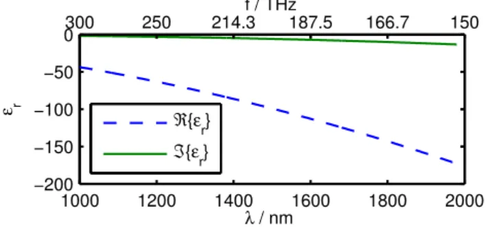
α0,α1,β0 andβ1are real-valued, and anej ωt time depen-dency is implied. Figure 1 exemplarily shows the real and imaginary part of the relative permittivity of silver in the in-frared range. The data from (Johnson and Christy, 1972) can be fitted by the parameter set ǫ∞=5, α0=0, α1=3.22e13, β0=1.96e32,β1=0 of a Drude approximation.
The imaginary part of the complex permittivity can be reinterpreted as a conductivity, and from the conductivity the skin-depth can easily be calculated. For instance, at a wavelength of 1.5 microns we obtain a skin-depth of 140 nm, which implies that we can not model thin sheets of a mate-rial like silver as a good or even perfect electrical conductor at optical frequencies.
3 Eigenmode formulation
3.1 Non-linear and polynomial eigenvalue problem In the following, we derive the non-linear eigenvalue formu-lation for structures with dispersive materials. For the sake of simplicity, we assume a homogeneous medium and begin in the continuous rather than the discrete regime. The eigen-mode formulation for the electrical field strengthE follows from Maxwell’s equations in frequency domain and reads
curl 1
µcurlE=ω
2ǫ(ω)E.
1000 1200 1400 1600 1800 2000 −200
−150 −100 −50 0
λ / nm
ε r
ℜ{εr} ℑ{ε
r}
300 250 214.3 187.5 166.7 150
f / THz
Fig. 1.Real and imaginary part of the relative permittivity of silver in the infrared range.
The dispersion of the permittivityǫ(ω)shall be given by a Drude model as motivated in Sect. 2:
ǫ(ω)=ǫ0
ǫ∞+
β0 j ωα1−ω2
. (3)
We insert Eq. (3) into Eq. (2) and obtain the complex, non-hermitian, polynomial eigenvalue problem (PEP) inω (ω3a3+ω2a2+ωa1+a0)E =0. (4) The coefficientsai are given by
a0= −j α1Acc, a1=ǫ0β0+Acc,
a2=j ǫ0ǫ∞α1, a3= −ǫ0ǫ∞, Acc =curl
1
µcurl.
3.2 Discrete formulation
The eigenvalue formulation is discretized using the finite in-tegration technique (FIT) (Weiland, 1977, 1996). In this very general framework Maxwell’s equations are transformed into algebraic equations – the Maxwell’s Grid Equations – which can be used further to formulate e.g. a discrete wave equa-tion. The degrees of freedom of the FIT approach are the so-called grid voltages⌢e, which are defined on the edges of a three-dimensional Cartesian grid. Finally, the discrete repre-sentation of the non-linear eigenvalue problem Eq. (2) reads
Acc⌢e=ω2Mε(ω)⌢e. (5)
Here, the large and sparse matrixAccis the curl-curl system
operator and includes the double curl operation as well as the permeability distribution of the structure. The diagonal ma-trixMεis the generalized permittivity operator. The searched
eigenvalue is the squared angular frequencyω2, and the field distribution is defined by the eigenvector⌢e
. The dimension of the problem isNe×Ne, withNethe number of grid edges.
In a straight forward manner, we can also find a discrete representation of the PEP Eq. (4) using FIT
9(ω)⌢e=(ω3A3+ω2A2+ωA1+A0)⌢e=0, (6)
where Ai are the spatially discretized coefficient matrices
corresponding to theai of Eq. (4). This representation also
supports an arbitrary inhomogeneous material distribution (including the dispersive permittivity), and it turns out that the usual facet-weighted averaging procedure at material in-terfaces does not need any special treatment. In FIT with Cartesian grids the matricesA3andA2are diagonal, andA1 andA0are sparse. The resulting PEP is complex and non-Hermitian.
4 Solver for polynomial eigenvalue problems
The PEP from Sect. 3.2 can be solved in different ways, and we briefly discuss four variants.
4.1 Fixed-point iteration
A first idea is to evaluateMε(ω)at a certain frequencyωiand
to solve a standard linear eigenvalue problem from Eq. (5) for the eigenfrequencyωi+1:
Acc⌢e=ωi2+1Mε(ωi)⌢e. (7)
This approach defines a fixed-point iteration process
ωi+1=8(ωi), where the operator8includes a solving step
of standard linear eigenvalue problem.
This scheme works well (but not very fast) in many cases. However, the proof of its convergence for general cases – e.g. using Banach’s fixed-point theorem – is quite challeng-ing due to the complex nature of the eigenvalue problem in-volved.
4.2 Linearization via companion matrix
A direct way to solve any PEP is to use the so-called compan-ion matrix of the PEP. A PEP of orderican be recast into a generalized linear eigenvalue problem of the formAx=λBx, where
A=
0 I · · · 0
..
. ... . .. ... ..
. ... ... I −A0−A1· · · −Ai−1
, (8)
B=
I
. ..
I Ai
, x=
⌢e
ω⌢e .. . ωi−1⌢
e
.
4.3 Newton-type methods for PEPs
The Newton method for polynomial eigenvalue problems may be regarded as a generalization of the method of inverse iteration (Schreiber, 2008). The algorithm yields one eigen-pair at a time and is based on a functionf of the eigenvector uand the eigenvalueω
f
u ω
=
9(ω)u wHu−1
. (9)
It includes the matrix polynomial9(ω)from Eq. (6) and a normalization vectorw, which has to be chosen such that wHu=1 holds throughout the iteration. The first derivative of Eq. (9) is given by the Jacobian
J
u ω
=
9(ω) 9′(ω)u
wH 0
(10) where9′(ω)denotes the derivation of Eq. (6). For a given
starting guess of the eigenpair(u0, ω0), the Newton correc-tion at stepiis defined by
J
ui ωi
1ui+1 1ωi+1
= −f
ui ωi
(11) and
ui+1=ui+1ui+1, ωi+1=ωi+1ωi+1.
Therefore, the linear system Eq. (11) has to be solved in each iteration step. The Newton algorithm is terminated if the norm of the residual
r =9(ω)u (12)
is sufficiently small.
4.4 Jacobi-Davidson algorithm for PEPs
The PEP in the form Eq. (6) can also be solved using a Jacobi-Davidson algorithm (JD) (Sleijpen et al., 1996; Bai et al., 2000). This method is intended to find one or more interior eigenvalues of the spectrum near a given targetω0.
The main idea within the JD method is to project the PEP on a low-dimensional orthogonal subspace V, which leads to a low-dimensional PEP with coefficient matrices Mi=V∗AiV. The low-dimensional PEP can be solved by the
companion matrix approach from Sect. 4.2 and any method for generalized eigenvalue problems. The low-dimensional eigenvectors is expanded to full size again, u=Vs, which leads to the current approximative eigenvector u. Sinceu is an approximation, the residual Eq. (12) has to be calcu-lated, and the process stops if the norm ofr is sufficiently small. Since this typically does not occur after the first iter-ation step, a so-called correction equiter-ation is formulated and solved, which produces an additional vector, which extends the subspace.
This procedure is repeated until convergence. The compu-tationally most expensive task inside the JD iteration is the solution of the correction equation, which reads
I−pu
∗
u∗p
9(θ )(I−uu∗)t= −r. (13)
Here,9is the polynomial from Eq. (6) evaluated at the last, best estimation θ (namely the Ritz value), t is the correc-tion vector, r the residual, u=Vs the best actual approxi-mation of the searched eigenvector, and p=9′(θ )
. In the beginning of the JD process the user-defined targetω0 may be more accurate than an extracted Ritz value. Therefore we set p=9′(ω
0)until the residual is below a predefined tolerance, in order to get a better correction vectort. (This was proposed in (Hochstenbach and Sleijpen, 2008).) For the solution of the correction Eq. (13) we use a preconditioned bicgstab(l) method (Sleijpen and Fokkema, 1993). As pre-conditioner we use an LU decomposition of the polynomial evaluated at the target valueω0. Therefore the LU decompo-sition has to be established only once per JD run.
4.5 Validation
A simple way to validate a specific implementation from the Newton method from Sect. 4.3 or the JD method from Sect. 4.4 is to go back to the fixed-point formulation in Eq. (7) and to execute one single step of the iteration. In all numerical tests our results yield accuracies in the range of numerical noise.
5 Numerical example
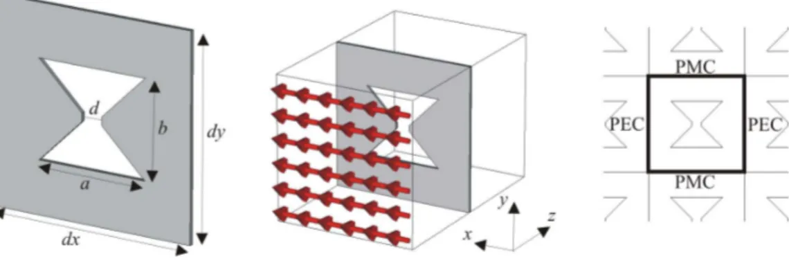
As an example we take a bow tie slot antenna which can be regarded as a resonator at optical wavelengths. A potential application is in spectroscopy where field confinement and focusing is desirable. An extensive study can be found e.g. in Guo et al., 2008.
5.1 Setup
Fig. 2. Bow tie antenna structure witha=270 nm,b=240 nm,d=50 nm and thickness oft=10 nm. The transversal dimensions are dx=dy=500 nm. The polarization of the incident TEM wave and the resulting transversal boundary conditions are shown at the center and at the right.
150 200 250
10 15 20 25
Target frequency / THz
Number of iterations
JD Newton
Fig. 3.Number of iterations of the JD and Newton method to con-verge for different target frequenciesω0.
antennas illuminated by a plane wave, the transversal bound-ary conditions are chosen to be perfectly electric and per-fectly magnetic conducting (cf. Fig. 2). In propagation di-rection we apply Berenger’s perfectly matched layer (PML) (Berenger, 1994) to truncate the computational domain ap-propriately. The PML itself consists of frequency dependent materials, but here we evaluate the PML once at our start-ing frequencyω0 instead of including its frequency depen-dence into the eigenvalue formulation. Nevertheless, to de-termine the eigenfrequency of the bow tie antenna, a com-plex non-Hermitian polynomial eigenvalue problem has to be solved, and we compare the results of the Newton method from Sect. 4.3 to those of the JD method from Sect. 4.4, both of them implemented in MATLAB. Convergence is supposed to be reached when the norm of the residual Eq. (12) is less than 1e-9.
5.2 Results
An estimation of the eigenfrequency can be obtained, e.g., by measurements or a scattering parameter simulation, see
150 200 250
0 200 400 600
Target frequency / THz
Found eigenfrequency / THz
JD Newton
Fig. 4. Resulting eigenvalues of the JD and Newton method for different target frequenciesω0.
(Guo et al., 2008) for details. In our case the searched eigen-frequency is at 192.4 THz.
Figure 3 shows the number of iterations needed by the Jacobi-Davidson and Newton method to generate an eigen-pair for different target frequenciesω0. In almost all cases the Jacobi-Davidson method needs less iterations than the New-ton method for our specific setup. However, it is questionable which eigenpairsare actually found
Figure 4 shows the eigenfrequencies generated by the Jacobi-Davidson and Newton method for different target fre-quenciesω0. It turns out that the result of the Newton method strongly depends on the chosen target frequencyω0for the first step of Eq. (11). On the contrary the Jacobi-Davidson method reliably generates the same eigenvalue also for less accurately chosen target frequencies.
Figure 5 shows the time needed for the computation of the eigenfrequency (including only those runs which led to the desired eigenvalue of 192.4 THz). Again the JD method out-performs the Newton approach in all cases considered here.
160 180 200 220 240 20
40 60 80
Target frequency / THz
Needed time / sec
JD Newton
Fig. 5. Computation times of JD and Newton method for target frequencies, which lead to the searched eigenvalue.
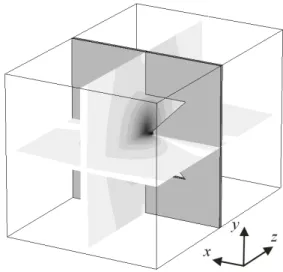
orientated inx-direction (like the incident plane wave) and is concentrated within the slot of the bow tie antenna as pro-posed in the literature.
6 Conclusions
After a review of the behavior of metals at optical frequen-cies, an eigenfrequency formulation which is capable to deal with frequency dispersive materials has been presented. The formulation is based on the finite integration technique and leads to a polynomial eigenvalue problems (PEP). Four strategies to solve this PEP have been presented and tested. As a numerical example we have used a bow tie slot antenna (Guo et al., 2008) which consists of silver and operates at a wavelengths around 1.5 microns. We have computed its resonance frequency and compared the Newton method and the Davidson method. It turns out that the Jacobi-Davidson method is more robust in terms of poorly chosen target frequencies and also faster at least in our implementa-tion.
If the match of measurement data of material properties requires higher order polynomial functions, our formulation of Sect. 3 can easily be extended and will lead to higher order matrix polynomials.
References
Bai, Z., Demmel, J., Dongarra, J., Ruhe, A., and van der Vorst, H.: Templates for the Solution of Algebraic Eigenvalue Problems: A Practical Guide, SIAM, Philadelphia, 2000.
Berenger, J.-P.: A perfectly matched layer for the absorption of elec-tromagnetic waves, J. Comput. Phys., 114, 185–200, 1994. Computer Simulation Technology AG (CST): CST Studio Suite
2008, http://www.cst.com, 2008.
Guo, H., Meyrath, T. P., Zentgraf, T., Liu, N., Fu, L., Schweizer, H., and Giessen, H.: Optical resonances of bowtie slot an-tennas and their geometry and material dependence, Opt. Ex-press, 16, 7756–7766, http://www.opticsexpress.org/abstract. cfm?URI=oe-16-11-7756, 2008.
Fig. 6. Contour plot of the field distribution of the eigensolution at 192.4 THz: Thex-component of the electrical field strength is confined within the slot of the bow tie antenna.
Hochstenbach, M. E. and Sleijpen, G. L. G.: Harmonic and refined Rayleigh-Ritz for the polynomial eigenvalue problem, Numeri-cal Linear Algebra with Applications, 15, 35–54, 2008. Johnson, P. B. and Christy, R. W.: Optical Constants of the Noble
Metals, Phys. Rev. B., 6, 4370–4379, 1972.
Ordal, M. A., Long, L. L., Bell, R. J., Bell, S. E., Bell, R. R., R. W. Alexander, J., and Ward, C. A.: Optical properties of the metals Al, Co, Cu, Au, Fe, Pb, Ni, Pd, Pt, Ag, Ti, and W in the infrared and far infrared, Appl. Opt., 22, 1099–1119, http://ao.osa.org/abstract.cfm?URI=ao-22-7-1099, 1983. Palik, E. D.: Handbook of Optical Constants of Solids , 1997. Rakic, A. D., Djuriˇsic, A. B., Elazar, J. M., and Majewski, M. L.:
Optical Properties of Metallic Films for Vertical-Cavity Opto-electronic Devices, Appl. Opt., 37, 5271–5283, http://ao.osa.org/ abstract.cfm?URI=ao-37-22-5271, 1998.
Schreiber, K.: Nonlinear Eigenvalue Problems: Newton-type Meth-ods and Nonlinear Rayleigh Functionals, Ph.D. thesis, TU Berlin, http://nbn-resolving.de/urn:nbn:de:kobv:83-opus-18754, 2008.
Sleijpen, G. L. G. and Fokkema, D. R.: Bi-CGSTAB(l) for linear equations involving unsymmetric matrices with complex spec-trum, Elec. Trans. Numer. Anal., 1, 11–32, 1993.
Sleijpen, G. L. G., Booten, A. G. L., Fokkema, D. R., and der Vorst, H. A. V.: Jacobi-Davidson type methods for generalized and polynomial eigenproblems, BIT, 36, 595–633, 1996. Weiland, T.: Eine Methode zur L¨osung der Maxwellschen
Gle-ichungen f¨ur sechskomponentige Felder auf diskreter Basis, Archiv f¨ur Elektronik und ¨Ubertragungstechnik, 31, 116–120, 1977.