www.atmos-chem-phys.net/16/15709/2016/ doi:10.5194/acp-16-15709-2016
© Author(s) 2016. CC Attribution 3.0 License.
Long-term observations of cloud condensation nuclei in the Amazon
rain forest – Part 1: Aerosol size distribution, hygroscopicity, and
new model parametrizations for CCN prediction
Mira L. Pöhlker1, Christopher Pöhlker1, Florian Ditas1, Thomas Klimach1, Isabella Hrabe de Angelis1, Alessandro Araújo2, Joel Brito3,a, Samara Carbone3,b, Yafang Cheng1, Xuguang Chi1,c, Reiner Ditz1,
Sachin S. Gunthe4, Jürgen Kesselmeier1, Tobias Könemann1, Jošt V. Lavriˇc5, Scot T. Martin6, Eugene Mikhailov7,
Daniel Moran-Zuloaga1, Diana Rose8, Jorge Saturno1, Hang Su1, Ryan Thalman9,d, David Walter1, Jian Wang9,
Stefan Wolff1,10, Henrique M. J. Barbosa3, Paulo Artaxo3, Meinrat O. Andreae1,11, and Ulrich Pöschl1
1Multiphase Chemistry and Biogeochemistry Departments, Max Planck Institute for Chemistry, 55020 Mainz, Germany 2Empresa Brasileira de Pesquisa Agropecuária (EMBRAPA), Trav. Dr. Enéas Pinheiro, Belém, PA, 66095-100, Brazil 3Institute of Physics, University of São Paulo, São Paulo, 05508-900, Brazil
4EWRE Division, Department of Civil Engineering, Indian Institute of Technology Madras, Chennai 600036, India 5Department of Biogeochemical Systems, Max Planck Institute for Biogeochemistry, 07701 Jena, Germany 6School of Engineering and Applied Sciences, Harvard University, Cambridge, MA 02138, USA
7St. Petersburg State University, 7/9 Universitetskaya nab, St. Petersburg, 199034, Russia
8Institute for Atmospheric and Environmental Research, Goethe University Frankfurt am Main, 60438 Frankfurt, Germany 9Biological, Environmental & Climate Sciences Department, Brookhaven National Laboratory, Upton, NY 11973, USA 10Instituto Nacional de Pesquisas da Amazonia (INPA), Manaus, 69083-000, Brazil
11Scripps Institution of Oceanography, University of California San Diego, La Jolla, CA 92037, USA anow at: Laboratory for Meteorological Physics, University Blaise Pascal, Clermont-Ferrand, France bnow at: Federal University of Uberlândia, Uberlândia-MG, 38408-100, Brazil
cnow at: Institute for Climate and Global Change Research & School of Atmospheric Sciences, Nanjing University,
Nanjing, 210093, China
dnow at: Department of Chemistry, Snow College, Richfield, UT 84701, USA
Correspondence to:Mira L. Pöhlker ([email protected])
Received: 16 June 2016 – Published in Atmos. Chem. Phys. Discuss.: 23 June 2016 Revised: 18 October 2016 – Accepted: 7 November 2016 – Published: 20 December 2016
Abstract. Size-resolved long-term measurements of atmo-spheric aerosol and cloud condensation nuclei (CCN) con-centrations and hygroscopicity were conducted at the re-mote Amazon Tall Tower Observatory (ATTO) in the cen-tral Amazon Basin over a 1-year period and full seasonal cycle (March 2014–February 2015). The measurements pro-vide a climatology of CCN properties characteristic of a re-mote central Amazonian rain forest site.
The CCN measurements were continuously cycled through 10 levels of supersaturation (S =0.11 to 1.10 %) and span the aerosol particle size range from 20 to 245 nm. The mean critical diameters of CCN activation range from
43 nm atS=1.10 % to 172 nm at S=0.11 %. The particle hygroscopicity exhibits a pronounced size dependence with lower values for the Aitken mode (κAit=0.14±0.03), higher
values for the accumulation mode (κAcc=0.22±0.05), and
an overall mean value ofκmean=0.17±0.06, consistent with
high fractions of organic aerosol.
concentra-tion. We find that the variability in the CCN concentrations in the central Amazon is mostly driven by aerosol particle number concentration and size distribution, while variations in aerosol hygroscopicity and chemical composition matter only during a few episodes.
For modeling purposes, we compare different approaches of predicting CCN number concentration and present a novel parametrization, which allows accurate CCN predictions based on a small set of input data.
1 Introduction
1.1 Atmospheric aerosols and clouds
In our current understanding of the Earth’s climate system and its man-made perturbation, the multiscale and feedback-rich life cycles of clouds represent one of the largest uncer-tainties (Boucher et al., 2013; Stevens et al., 2016). Accord-ingly, the adequate and robust representation of cloud prop-erties is an Achilles’ heel in climate modeling efforts (Bony et al., 2015). Atmospheric aerosols are a key ingredient in the life cycle of clouds (known as aerosol indirect effect) as they affect their formation, development, and properties by acting as cloud condensation nuclei (CCN) and ice nuclei (IN) (Lohmann and Feichter, 2005; Rosenfeld et al., 2008). Aerosol particles can originate from various natural and an-thropogenic sources and span wide ranges of concentration, particle size, composition, as well as chemical and phys-ical properties (Pöschl, 2005). Their activation into cloud droplets depends on their size, composition, and mixing state as well as the water vapor supersaturation (e.g., Köhler, 1936; Dusek et al., 2006; McFiggans et al., 2006; Andreae and Rosenfeld, 2008; Su et al., 2010). The microphysical link between clouds and aerosol has been the subject of mani-fold and long-term research efforts. On one hand, the cycling of CCN as well as their relationship to the aerosol population has been studied in a variety of field experiments worldwide (e.g., Gunthe et al., 2009; Rose et al., 2010; Jurányi et al., 2011; Paramonov et al., 2015). On the other hand, the knowl-edge obtained from the growing body of field data has been translated into different parametrization strategies that repre-sent the cloud–aerosol microphysical processes in modeling studies (e.g., Nenes and Seinfeld, 2003; Petters and Kreiden-weis, 2007; Su et al., 2010; Deng et al., 2013; Mikhailov et al., 2013).
1.2 Amazon rain forest and its hydrological cycle The Amazon rain forest is a unique and important ecosys-tem for various reasons such as its high density and diversity of life, its role as major carbon storage, and its large recling rate of energy and water in the Earth’s hydrological cy-cle (Brienen et al., 2015; Gloor et al., 2015; Olivares et al., 2015; Yáñez-Serrano et al., 2015). In times of global change,
the man-made disturbance and pressure on this ecosystem have strongly increased and have started a transition of the Amazon into an uncharted future (Davidson et al., 2012; Lawrence and Vandecar, 2015). In the context of atmospheric composition, the Amazon is unique since it represents one of the last terrestrial locations worldwide that allows – at least for part of the year – to investigate an relatively undis-turbed state of the atmosphere in the absence of major an-thropogenic pollution (Roberts et al., 2001; Andreae, 2007; Andreae et al., 2012; Hamilton et al., 2014).
Overall, the troposphere over the Amazon is defined by the alternation of a relatively clean wet season and a polluted dry season, as outlined in more detail in previous studies (e.g., Martin et al., 2010b; Andreae et al., 2012, 2015; Mishra et al., 2015). In this paper, we use the following classifica-tion of the Amazonian seasons1: (i) the wet season typically spans February to May and shows the cleanest atmospheric state, (ii) the transition period from wet to dry season typi-cally spans June and July, (iii) the dry season months August to November show the highest pollution levels, and (iv) the transition period from dry to wet season spans December and January (Andreae et al., 2015; Moran-Zuloaga et al., 2017).
A lively discussed aspect of the Amazonian hydrological cycle is the potential impact of changing aerosol regimes, which oscillate between polluted and pristine extremes, on the development of clouds and precipitation (e.g., Roberts et al., 2003; Andreae et al., 2004; Rosenfeld et al., 2008). A va-riety of pollution-induced changes in cloud properties, such as increased cloud drop concentrations with a corresponding decrease of their average size, intense competition for wa-ter vapor, and thus a deceleration of drop growth rates, sup-pression of supersaturation, reduced coalescence of smaller droplets, increased cloud depths as well as an invigoration of cloud dynamics and rain, are well documented (e.g., Koren et al., 2004, 2012; Freud et al., 2008).
Overall, the aforementioned observations indicate that in-creasing aerosol concentrations can have substantial impacts on spatial and temporal rainfall patterns in the Amazon (e.g., Martins et al., 2009a; Reutter et al., 2009). In view of the globally increasing pollution levels and the ongoing defor-estation in the Amazon, pollution-triggered perturbations of the hydrological cycle are discussed as potential major threats to the Amazonian ecosystem, its forest structure, sta-bility, and integrity (e.g., Coe et al., 2013; Junk, 2013).
1.3 Previous CCN measurements in the Amazon Ground-based and airborne CCN measurements have been conducted in a number of field campaigns in the Amazon Basin as outlined below in chronological order, constituting the baseline and context for the present study.
1998: Roberts and coworkers (Roberts et al., 2001; Roberts et al., 2002) conducted the first CCN measurements in the Amazon in the context of the LBA/CLAIRE-98 campaign (ground-based, Balbina site, March and April 1998) and pointed out that under clean conditions the CCN concentrationNCCN(S) (at a certain
supersatura-tion S) in the “green ocean” Amazon is surprisingly similar to conditions in the maritime “blue ocean” at-mosphere. Regarding the low naturalNCCN(S), which
is dominated by mostly organic particles, they further suggested that cloud and precipitation properties may react sensitively to pollution-induced increases of the total aerosol load.
1999: In the context of the LBA-EUSTACH campaign in 1999, ground-based CCN measurements at three dif-ferent sites in the Amazon Basin were conducted (An-dreae et al., 2002; Roberts et al., 2003). This was the first study on CCN properties and cloud dynamics un-der the influence of strong biomass burning emissions in the Amazon.
2001: In the follow-up study LBA/CLAIRE-2001 in July 2001, ground-based (Balbina site) and airborne mea-surements (around Manaus) were conducted. For the ground-based study, Rissler et al. (2004) combined a hy-groscopicity tandem differential mobility analyzer (HT-DMA) with CCN measurements, focusing on the CCN-relevant water-soluble fraction in the particles, and pro-vided a CCN closure and parametrization for model ap-proaches. In addition, an airborne analysis of the aerosol and CCN properties was conducted, focusing on the contrast between the Amazonian background air and the Manaus plume (Kuhn et al., 2010).
2002: Subsequently, in the course of the LBA-SMOCC-2002 campaign in southern Brazil during major biomass burning episodes (Rondônia state, September and Octo-ber 2002), ground-based and airborne CCN measure-ments were performed (Vestin et al., 2007; Martins et al., 2009b). A major finding of this study was that the CCN efficiency of natural biogenic and man-made py-rogenic (cloud-processed) aerosols is surprisingly sim-ilar (Andreae et al., 2004). Furthermore, NCCN(0.5 %)
was found as a valuable predictor for the required cloud depth of warm rain formation, which is an important property for cloud dynamics (Freud et al., 2008). 2008: During the AMAZE-08 campaign (ground-based,
ZF2 site, February and March 2008), the first
size-resolved CCN measurements in the Amazon were con-ducted (Gunthe et al., 2009; Martin et al., 2010a). These studies report that aerosol particles in the Aitken and ac-cumulation modes, which represent the CCN-relevant size range, predominantly contain organic constituents and thus have comparably low hygroscopicity levels. The observed hygroscopicity parameter κ ranges be-tween 0.1 and 0.2, which corresponds to the typical hy-groscopicity of secondary organic aerosol (SOA) (An-dreae and Rosenfeld, 2008).
2010/11: During several short observational periods, Almeida et al. (2014) measured total CCN concentra-tions around the city of Fortaleza in northeast Brazil. The selected measurement locations receive wind from changing directions. Accordingly, the response of the CCN population to marine, urban, and rural air masses was investigated.
2013: Recently, Whitehead et al. (2016) reported results from further short-term, size-resolved CCN and HT-DMA measurements that were conducted north of Man-aus (ground-based, ZF2 site, July 2013) as part of the Brazil–UK network for investigation of Amazonian at-mospheric composition and impacts on climate (BUNI-AACIC) project. The results of this study agree well with Gunthe et al. (2009).
2014/15: As part of the international field campaign ob-servation and modeling of the green ocean Amazon (GoAmazon2014/5), size-resolved CCN measurements were conducted at three sites in and around Manaus: the Amazon Tall Tower Observatory (ATTO) site (T0a, pristine rain forest), which is discussed in the present study, the T2 site (in Manaus, urban environment), and the T3 site (rural site in the Manaus plume) (Martin et al., 2016; Thalman et al., 2017). All three size-resolved CCN measurements in the context of GoAmazon2014/5 took place in close collaboration. Moreover, CCN mea-surements were conducted onboard the G-1 aircraft dur-ing the GoAmazon2014/5 intensive observation periods IOP1 and IOP2 (Martin et al., 2016).
2014: Furthermore, as part of the German–Brazilian ACRIDICON (Wendisch et al., 2016) and CHUVA (Machado et al., 2014) projects, airborne CCN mea-surements were made over the entire Amazon Basin (September 2014). The results of this study are currently being analyzed for an upcoming publication and repre-sent an ideal complement to the long-term data of the present study.
to extrapolate the CCN activity in supersaturation regimes (Zhou et al., 2002; Rissler et al., 2006).
1.4 Aims and scope of this study
All of the previously published CCN measurements in the Amazon have been conducted over relatively short time pe-riods of up to several weeks. In addition, size-resolved CCN measurements are still sparse in the Amazon region. In this study, we present the first continuous, long-term, and size-resolved CCN data set from the Amazon Basin, which spans a full seasonal cycle and therefore represents the CCN prop-erties during contrasting seasonal conditions.
The focus of this study is on presenting major trends and characteristics of the CCN population in the Amazon Basin. Thus, our study contributes to a global inventory of CCN properties, representing this unique and climatically important ecosystem. We extract key CCN properties and parameters that help to include CCN predictions in the Ama-zon region into future modeling studies. Based on our data set, different parametrization strategies for CCN prediction are compared and discussed. Moreover, we present a novel and generalized CCN parametrization, which allows efficient modeling of CCN concentrations based on a minimal set of basic aerosol properties.
This paper represents part 1 of a comprehensive analy-sis of the CCN cycling in the central Amazon. It covers the overall trends and presents annually averaged CCN param-eters as well as characteristic differences in the CCN pop-ulation between the Amazonian seasons. A companion pa-per (Part 2) provides in-depth analyses of particularly inter-esting events through short-term case studies and aims for a more emission- and process-related understanding of the CCN variability (M. L. Pöhlker et al., 2017a).
2 Methods
2.1 Measurement site and period
The measurements reported in this study were conducted at the ATTO site (02◦08.602′S, 59◦00.033′W; 130 m a.s.l.), which is located in an untouched rain forest area in the cen-tral Amazon, about 150 km northeast of the city of Manaus, Brazil. An overview of the atmospheric, geographic, and eco-logical conditions at the ATTO site has been published re-cently by Andreae et al. (2015), where a detailed description of the aerosol setup for the long-term measurements can be found. The instrumentation for CCN measurements is part of a broad aerosol measurement setup, which also covers aerosol size and concentration, absorptivity, scattering, flu-orescence, as well as chemical composition (Andreae et al., 2015). The aerosol inlet is located at a height of 60 m, which is about 30 m above the forest canopy. The sample air is dried by silica gel diffusion dryers at the main inlet, which keeps the RH below 40 %. For the CCN setup, a second diffusion
dryer decreases the RH even further to <20 %, which en-sures reliable hygroscopicity measurements.
The CCN measurements are ongoing since the end of March 2014. This study covers the measurement period from the end of March 2014 to February 2015, representing almost a full seasonal cycle. Also, the measurement period overlaps with the international large-scale field campaign GoAma-zon2014/5 that was conducted in and around the city of Man-aus from 1 January 2014 through 31 December 2015. Dur-ing GoAmazon2014/5, comprehensive CCN measurements were conducted at different sites (see Sect. 1.3) (Martin et al., 2016). The ATTO site served as a clean background (T0a) site during GoAmazon2014/5. Furthermore, the mea-surement period of this study encompasses the German– Brazilian ACRIDICON-CHUVA field measurement cam-paign in September 2014 (Machado et al., 2014; Wendisch et al., 2016), where (non-size-resolved) CCN measurements at multiple supersaturation levels were performed onboard the high-altitude and long-range research aircraft (HALO) flying over the Amazon Basin.
2.2 Size-resolved CCN measurements
The number concentration of CCN was measured with a continuous-flow streamwise thermal gradient CCN counter (CCNC, model CCN-100, DMT, Boulder, CO, USA) (Roberts and Nenes, 2005; Rose et al., 2008b). The inlet flow rate of the CCNC was 0.5 L min−1with a sheath-to-aerosol flow ratio of 11. The water pump was operated at a rate of 4 mL h−1 corresponding to the CCNC setting of “low”
liq-uid flow. The supersaturation (S) of the CCNC was cycled through 10 differentS values between 0.11 and 1.10 % (see Table 1), which are defined by controlled temperature gra-dients inside the CCNC column. Particles with a critical su-persaturation (Sc)≤Sin the column are activated and form
water droplets. Droplets with diameters≥1 µm are detected by an optical particle counter (OPC) at the exit of the column. Size-resolved CCN activation curves (for nomenclature, see Sect. 2.3) were measured based on the concept of Frank et al. (2006), following the procedures in Rose et al. (2008a) and Krüger et al. (2014) by combining the CCNC with a dif-ferential mobility analyzer (DMA, model M, Grimm Aerosol Technik, Ainring, Germany). The DMA was operated with a sheath-to-aerosol flow ratio of 5. The DMA selects particles with a certain diameter (D) in the size range of 20 to 245 nm (sequence ofDvalue has been optimized for everyS), which are then passed into the two instruments: (i) the CCNC sys-tem and (ii) a condensation particle counter (CPC, model 5412, Grimm Aerosol Technik), which measures the number concentration of aerosol particles with selectedD(NCN(D)),
while the CCNC measures the number concentration of CCN with selected D for the given S(NCCN(S,D)). The cycle
through a full CCN activation curve (NCCN(S,D)/NCN(D))
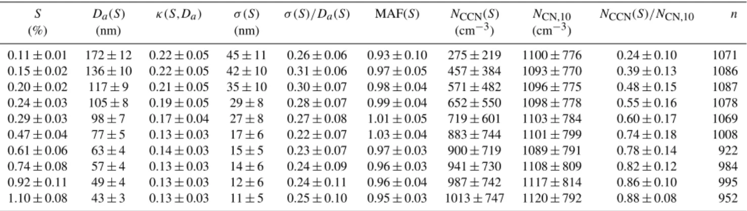
Table 1.Characteristic CCN parameters as a function of the supersaturationS, averaged over the entire measurement period: midpoint activation diameterDa(S), hygroscopicity parameterκ(S,Da), width of CCN activation curveσ(S), heterogeneity parameterσ(S)/Da(S), maximum activated fraction MAF(S), CCN number concentrationNCCN(S), total particle concentration (>10 nm)NCN,10, CCN efficiencies NCCN(S)/NCN,10, and number of data pointsn.Sis shown as set value±the experimentally derived deviation inS. All other values are given as arithmetic mean±1 standard deviation. All values are provided for ambient conditions (temperature∼28◦C; pressure∼100 kPa).
S Da(S) κ(S,Da) σ (S) σ (S)/Da(S) MAF(S) NCCN(S) NCN,10 NCCN(S)/NCN,10 n
(%) (nm) (nm) (cm−3) (cm−3)
0.11±0.01 172±12 0.22±0.05 45±11 0.26±0.06 0.93±0.10 275±219 1100±776 0.24±0.10 1071 0.15±0.02 136±10 0.22±0.05 42±10 0.31±0.06 0.97±0.05 457±384 1093±770 0.39±0.13 1086 0.20±0.02 117±9 0.21±0.05 35±10 0.30±0.07 0.98±0.04 571±482 1096±775 0.48±0.15 1087 0.24±0.03 105±8 0.19±0.05 29±8 0.28±0.07 0.99±0.04 652±550 1098±778 0.55±0.16 1078 0.29±0.03 98±7 0.17±0.04 27±8 0.27±0.08 1.01±0.05 719±601 1103±784 0.60±0.17 1069 0.47±0.04 77±5 0.13±0.03 17±6 0.22±0.07 1.03±0.04 883±744 1101±799 0.74±0.18 1008 0.61±0.06 63±4 0.14±0.03 15±5 0.23±0.07 0.97±0.03 900±719 1089±791 0.78±0.14 922 0.74±0.08 57±4 0.13±0.03 14±6 0.24±0.09 0.96±0.03 941±730 1108±809 0.82±0.12 984 0.92±0.11 49±4 0.13±0.03 12±6 0.24±0.11 0.96±0.04 987±742 1117±814 0.86±0.10 995 1.10±0.08 43±3 0.13±0.03 11±5 0.25±0.10 0.95±0.03 1013±747 1120±792 0.88±0.08 952
for every newSlevel. The completion of a full measurement cycle comprising CCN activation curves for 12–13 D val-ues (number of D depends onS) and 10 different S levels took∼4.5 h. The entire CCN system (including the CCNC, DMA, and CPC) was controlled by a dedicated LabVIEW (National Instruments, Munich, Germany) routine.
TheSlevels of the CCNC system were calibrated period-ically (March, May, and September 2014) using ammonium sulfate ((NH4)2SO4, Sigma Aldrich, St. Louis, MO, USA)
particles generated in an aerosol nebulizer (TSI Inc., Shore-view, MN, USA). The calibration procedure was conducted according to Rose et al. (2008b). All three calibrations gave consistent results and thus confirmed that the S cycling in the CCNC was very stable and reliable throughout the entire measurement period.
All concentration data presented here are given for am-bient conditions. During the entire measurement period, no significant fluctuations in temperature (∼28◦C) and pressure (∼100 kPa) were observed in the air-conditioned laboratory container.
2.3 Data analysis, error analysis, and nomenclature of CCN key parameters
The theoretical background and related CCN analysis pro-cedures are comprehensively described elsewhere (Petters and Kreidenweis, 2007; Rose et al., 2008a). For the present study, the following corrections were applied to the data set. (i) The CCN activation curves were corrected for sys-tematic deviations in the counting efficiency of the CCNC and CPC according to Rose et al. (2010). (ii) Usually, the double-charge correction of the CCN activation curve is con-ducted according to Frank et al. (2006). For this study, we developed the following alternative approach, which recon-structs the CCN efficiency curves based on data from an inde-pendent scanning mobility particle sizer (SMPS, TSI model
3080 with CPC 3772 operating with standard TSI software) at the ATTO site. The activation curve for everyD can be described by the following equation:
P
i
NCCN(S,Di)
P
i
NCN(Di) =
P
i
f (Di)·s (Di)·a(S,Di)
P
i
f (Di)·s (Di)
. (1)
The CCN size distribution (NCCN(S,D)) was calculated by
NCCN(S,D)=s (D)·a (S,D) . (2)
In this equation,s(D) represents the particle number size dis-tribution of the SMPS atD(10≤D≤450 nm).
The CCN efficiencies (NCCN(S)/NCN,10; for
nomencla-ture, see end of Sect. 2.3) have been calculated based on the integral concentration of CN with lower size cutoff Dcut=10 nm (NCN,10)2and CCN (NCCN(S)) as
NCCN(S)
NCN,10 =
R
DNCCN(S,D)·dD
R
Ds(D)·dD
. (3)
In addition to Da(S), the maximum activated fraction (MAF(S)) can be obtained froma(S,D). MAF(S) typically equals unity, except for completely hydrophobic particles (i.e., fresh soot). The third parameter that can be derived froma(S,D) is the width of the CCN activation curveσ(S), which strongly depends on Da(S). The ratio betweenσ(S) andDa(S) (σ(S)/Da(S)) is called heterogeneity parameter and can be used as an indicator for the chemical and geomet-ric diversity of the aerosol particles.
The error inSwas calculated based on the uncertainty ac-cording to the commonly used calibration procedure (Rose et al., 2008b). Overall, the error1SofSequals approximately 10 %; however, in the following analysis, we have used the specific1Svalues for everyS(see Table 1). The uncertainty of the selected D of the DMA (1D) was obtained as the mean width of the Gaussian fit of polystyrene latex (PSL) beads and equals 5.3 nm. ForNCCN(S,D) andNCN(D), the
standard error of the counting statistic was used. By Gaussian error propagation we determined 1(NCCN(S,D)/NCN(D))
and then repeated the data analysis for the upper and lower bounds (1±1)×(NCCN(D,S)/NCN(D)). The
result-ing relative errors of the values NCCN(S), NCN,10, and
NCCN(S)/NCN,10do not depend onSand equal 6 %. The
er-rors ofDa(S) andκ(S,Da)depend onSand can be described as
1Da(S)=Da(S)·(S·0.07+0.03) (4) 1κ (S,Da)=κ (S,Da)·(S·0.17+0.10). (5) Throughout this study, we observed a slight systematic de-viation of the results for the supersaturationS=0.47 %. This effect can be seen, for example, in MAF(0.47 %) values ex-ceeding unity in Fig. 1 andNCCN(0.47 %,D)/NCN(D) values
exceeding unity in Fig. 5. The effect persists even after ap-plying all aforementioned corrections to the data and is most pronounced during the dry season. Yet, since we did not find any evidence of these data being erroneous, we decided to keep them in the study.
2Note that N
CN,10 usually corresponds to the total CPC-detectable aerosol particle number concentration for the characteris-tic size distribution at the ATTO site because the parcharacteris-ticle population in the nucleation-mode range (i.e.,<10 nm) is negligibly small.
The use of certain terms in the context of CCN mea-surements is not uniform in the literature. For clarity, we summarize the key parameters and terms applied in this study as follows: (i) the valueNCCN(S,D)/NCN(D) is called
CCN activated fraction, while (ii) NCCN(S,D)/NCN(D)
plotted against D is called CCN activation curve; (iii) NCCN(S) plotted against S is called CCN spectrum;
(iv)NCCN(S)/NCN,Dcut at a certainSlevel is called CCN ef-ficiency; (v) NCCN(S)/NCN,Dcut plotted againstS is called CCN efficiency spectrum.
2.4 Aerosol mass spectrometry
In addition to the CCN measurements, aerosol chemical spe-ciation monitor (ACSM, Aerodyne Research Inc., Billerica, MA, USA) measurements are being performed at the ATTO site (Andreae et al., 2015). The ACSM routinely charac-terizes nonrefractory submicron aerosol species such as or-ganics, nitrate, sulfate, ammonium, and chloride (Ng et al., 2011). Particles are focused by an aerodynamic lens system into a narrow particle beam, which is transmitted through three successive vacuum chambers. In the third chamber, the particle beam is directed into a hot tungsten oven (600◦C) where the particles are flash vaporized, ionized with a 70 eV electron impact ionizer, and detected with a quadrupole mass spectrometer. In this study, a time resolution of 30 min was used. The measurements provide a total mass concentration of the chemical composition of the aerosol particles. Further details about the ACSM can be found in Ng et al. (2011). 2.5 Carbon monoxide measurements
Carbon monoxide (CO) measurements are conducted con-tinuously at the ATTO site using a G1302 analyzer (Picarro Inc. Santa Clara, CA, USA). The experimental setup from the point of view of functioning and performance is a duplication of the system described in Winderlich et al. (2010).
3 Results and discussion
3.1 Time series of CCN parameters for the entire measurement period
Over the entire measurement period from 25 March 2014 to 5 February 2015 we recorded size-resolved CCN activa-tion curves at 10 different levels of water vapor supersat-urationS with an overall time resolution of approximately 4.5 h. A total of 10 253 CCN activation curves were fitted and analyzed to obtain parameters of CCN activity as de-tailed above (Sect. 2.3). Table 1 serves as a central refer-ence in the course of this study and summarizes the annual mean values and standard deviations of the following key pa-rameters, resolved byS:Da(S),κ(S,Da),σ(S),σ(S)/Da(S), MAF(S),NCCN(S), NCN,10, andNCCN(S)/NCN,10. In Fig. 1,
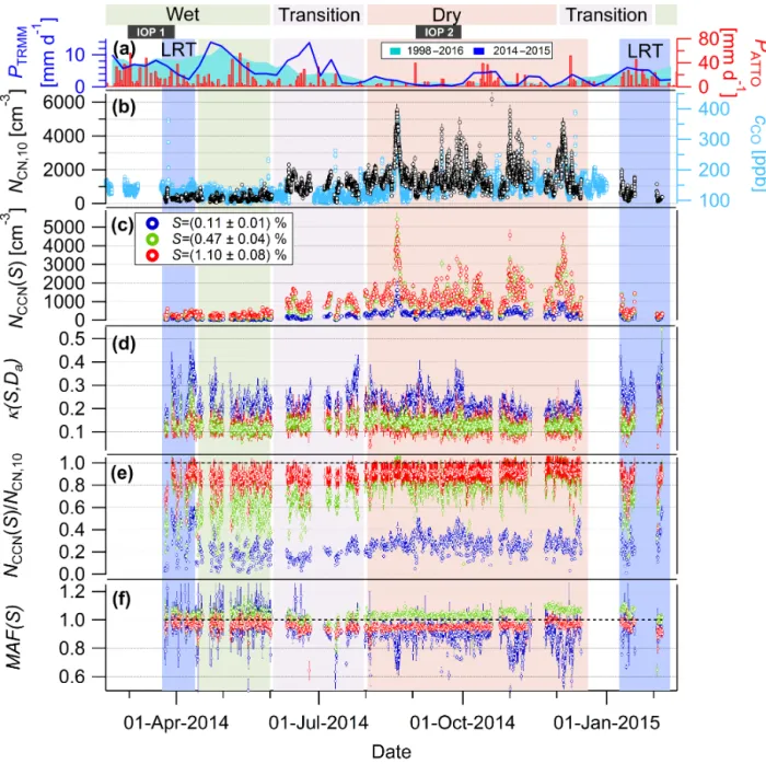
se-Figure 1.Seasonal trends in time series of precipitation rateP, total aerosol concentrationNCN,10, carbon monoxide mole fraction (cCO), and CCN key parameters for three selected supersaturationsSfor the entire measurement period (shown in original time resolution).(a) Pre-cipitation rates from tropical rainfall measuring mission (TRMM)PTRMMand in situ measurements at the ATTO sitePATTO. ThePTRMM seasonal cycles are derived from an area upwind of the ATTO site (59.5◦W, 2.4◦N, 54.0◦W, 3.5◦S), covering a long-term period from 1 Jan-uary 1998 to 30 June 2016 (aqua shading), and the period of the CCN measurements from 1 March 2014 to 28 FebrJan-uary 2015 (blue line). (b)Time series of pollution tracersNCN,10andcCO.(c)CCN concentrationsNCCN(S),(d)hygroscopicity parameterκ(S,Da),(e)CCN efficienciesNCCN(S)/NCN,10, and(f)maximum activated fraction MAF(S). Three different types of shading represent (i) the seasonality in the Amazon atmosphere according to Andreae et al. (2015) (wet vs. dry seasons with transition periods, illustrated at the top of the graph), (ii) periods of IOP1 and IOP2 during GoAmazon2014/5, (iii) seasonal periods of interest in context of the present study as defined in Sect. 3.3 (shading in background of time series).
ries over the entire measurement period to provide a general overview of their temporal evolution and variability. Concen-tration time series of the pollution tracersNCN,10and CO are
added to illustrate the pollution seasonality at the ATTO site.
anomalies due to teleconnections with the Atlantic and/or Pacific sea surface temperatures (SSTs) (Fu et al., 2001; Fernandes et al., 2015). The most prominent example here is the El Niño–Southern Oscillation (ENSO) and its vari-ous impacts on the Amazonian ecosystem (e.g., Asner et al., 2000; Ronchail et al., 2002). For the measurement pe-riod, the Oceanic Niño Index (ONI) ranged between −0.4 and 0.6◦C, confirming that only towards the end of the mea-surement period a slightly positive anomaly was observed.3 In Fig. 1a, satellite data from the tropical rainfall measure-ment mission (TRMM) are presented for the area around the ATTO site. The TRMM data are provided for an extended time period (January 1998 until June 2016) and, for com-parison, for the CCN measurement period (March 2014 un-til February 2015). This comparison shows that the 2014/15 precipitation rates do not deviate substantially from the 18-year average data, and thus further confirms that the measure-ment period can be regarded as a typical year with typical seasons and no pronounced hydrological anomalies.
Figure 1b displays the characteristic seasonal cycle in NCN,10 and the CO mole fraction (cCO). Both
pollu-tion tracers reach their maxima during the dry season (NCN,10=1400±710 cm−3; cCO=144±45 ppb), whereas
the lowest values are observed during the wet season (NCN,10=285±131 cm−3; cCO=117±12 ppb) (given as
mean±1 standard deviation). An obvious feature of the dry season months is the occurrence of rather short and strong peaks (reaching up to NCN,10= ∼5000 cm−3;
cCO= ∼400 ppb) on top of elevated background pollution
levels. The pronounced peaks originate from biomass burn-ing plumes, which impact the ATTO site for comparatively short periods (a few hours up to several days). Selected events are discussed in detail in M. L. Pöhlker et al. (2017a). Figure 1c shows that NCCN(S) follows the same overall
trends. A rather close correlation between NCCN(S) and
NCN,10 as well as NCCN(S) and cCO can be observed, as
pointed out in previous studies (Andreae, 2009; Kuhn et al., 2010). Figure 1d displays theκ(S,Da)time series for three exemplarySlevels. It shows that theκ(S,Da)values, which provide indirect information of the particles’ chemical com-position, are remarkably stable throughout the year (see also standard deviations of κ(S,Da)in Table 1). This illustrates that the dry season maximum inNCCN(S) is mainly related
to the overall increase inNCN,10, and not to substantial
varia-tions in aerosol composition and thereforeκ(S,Da). The lev-els of the threeκ(S,Da)time series, with their corresponding Da(S), provide a first indication thatκ(S,Da)shows a clear size dependence, as further discussed in Sect. 3.2. The
pro-3For the ONI data and specific information on the ref-erence area and time frame, refer to National Oceanic and Atmospheric Administration (NOAA)/National Weather Service, 2016. Historical El Niño/La Niña episodes (1950–present) are available at http://www.cpc.ncep.noaa.gov/products/analysis_ monitoring/ensostuff/ensoyears.shtml (last access: 1 October 2016).
nounced (but rather rare) “spikes” inκ(S,Da)(i.e., in April and August) as well as various other specific events in this time series are analyzed in detail in the companion Part 2 pa-per (M. L. Pöhlker et al., 2017a). Figure 1e gives an overview of the CCN efficienciesNCCN(S)/NCN,10 (for three S
lev-els) and its seasonal trends. This representation shows con-tinuously high fractions of cloud-active particles for higher S(e.g., NCCN(1.10 %)/NCN,10>0.9) throughout the entire
measurement period with almost no seasonality. For interme-diateS, such as 0.47 %, the values ofNCCN(0.47 %)/NCN,10
range from 0.6 to 0.9 and reveal a noticeable seasonal cy-cle, with the highest levels during the dry season. Further-more,NCCN(0.11 %)/NCN,10is mostly below 0.4, with clear
seasonal trends. These observations can be explained by the characteristic aerosol size distribution at the ATTO site (An-dreae et al., 2015), which (i) is dominated by particles in the Aitken (annually averaged peakDAitat∼70 nm) and
accu-mulation modes (annually averaged peakDAccat∼150 nm),
(ii) shows a sparse occurrence of nucleation-mode parti-cles (<30 nm), and (iii) reveals a clear seasonality in the relative abundance of Aitken and accumulation modes (see Sect. 3.3 and Fig. 6). Thus, the higher dry season abundance of accumulation-mode particles, which are more prone to act as CCN, results in higherNCCN(S)/NCN,10 levels,
particu-larly at lowerS.
Analogous NCCN(S)/NCN results from other
continental background sites have been pub-lished previously: for example, Levin et al. (2012) reported NCCN(0.97 %)/NCN=0.4–0.7,
NCCN(0.56 %)/NCN=0.25–0.5, and NCCN(0.14 %)/NCN
<0.15 for a semi-arid Rocky Mountain site. Jurányi et al. (2011) reported NCCN(1.18 %)/NCN,16=0.6–
0.9, NCCN(0.47 %)/NCN,16=0.2–0.6, and
NCCN(0.12 %)/NCN,16<0.25 for the high alpine
1.0 0.8 0.6 0.4 0.2 0.0
N
CCN(
S,D
)/
N
CN(
D
)
250 200
150 100
50 0
Diameter [nm]
S=(0.11±0.01) % S=(0.15±0.02) % S=(0.20±0.02) % S=(0.24±0.03) % S=(0.29±0.03) % S=(0.47±0.04) % S=(0.61±0.06) % S=(0.74±0.08) % S=(0.92±0.11) % S=(1.10±0.08) %
Figure 2. CCN activation curves for all measured S lev-els (S=0.11–1.10 %), averaged over the entire measurement period. Data points represent arithmetic mean values. For
NCCN(S,D)/NCN(D), the standard error is plotted, which is very small (due to the large number of scans with comparatively small variability) and therefore not perceptible in this representation. For the diameter,D, the error bars represent the experimental error as specified in Sect. 2.3. The grey vertical band represents the posi-tion of the Hoppel minimum (including error range) for the annual mean number size distribution (compare to Fig. 3). Dashed lines provide visual orientation and indicate 0, 50, and 100 % activation. The value at 50 % activation is used for calculation of the hygro-scopicity parameterκ(S,Da). The lines connecting the data points merely serve as visual orientation.
The MAF(S) time series in Fig. 1f represents a valuable additional parameter to determine the abundance of “poor” CCN (i.e., aerosol particles that are not activated into CCN within the tested S range). For higherS (i.e.,S >0.11 %), MAF(S) is close to unity over the whole year. In contrast, MAF(0.11 %) fluctuates around unity during the wet season months; however, it drops below unity during the biomass-burning-impacted dry season and subsequent transition pe-riod. For some episodes, MAF(S) shows very pronounced dips, as further discussed in the Part 2 study (M. L. Pöhlker et al., 2017a).
3.2 Annual means of CCN activation curves and hygroscopicity parameter
Figure 2 displays the annual mean CCN activation curves for all S levels. Thus, it represents an overall characterization of the particle activation behavior, which means that for de-creasingSlevels the activation diameter,Da(S), increases. In other words, everyS corresponds to a certain (and to some extent typical)Da(S) range, where particles start to become activated (see Table 1). As an example, relatively highS con-ditions (0.47–1.10 %) yield substantial activation already in the Aitken-mode range, while low S levels (0.11–0.29 %) correspond to activation of larger particles, mostly in the
ac-cumulation mode. Note that S levels in convective clouds rarely exceed 1.0 %, but that in the presence of precipitation higherSvalues are possible (Cotton and Anthes, 1989). The step from the activation curves atS=0.47 % toS=0.29 % relates to the position of the characteristic Hoppel minimum (at 97 nm for the annual mean size distribution; see Table 2) between Aitken and accumulation mode in the bimodal size distribution. Thus, the step toS=0.47 % represents the onset of significant activation in the Aitken-mode size range.
A different representation of these observations is dis-played in Fig. 3, which shows the bimodally fitted (bi-modal logarithmic normal distribution, R2=0.99) an-nual mean NCN(D) size distribution. In this annual
aver-age representation, the Aitken-mode maximum is located at DAit=69±1 nm, the accumulation-mode maximum at
DAcc=149±2 nm, and both are separated by the Hoppel
minimum (compare to Table 2) (Hoppel et al., 1996). Fur-thermore, Fig. 3 clearly shows that different κ(S,Da) val-ues are retrieved for the Aitken (κAit=0.14±0.03) vs. the
accumulation-mode size range (κAcc=0.22±0.03). This
in-dicates that Aitken- and accumulation-mode particles have different hygroscopicities and thus different chemical com-positions. In this case, Aitken-mode particles tend to be more predominantly organic (close to κ=0.1) than the accumulation-mode particles, which tend to contain more inorganic species (i.e., ammonium, sulfates, potassium) (Prenni et al., 2007; Gunthe et al., 2009; Wex et al., 2009; C. Pöhlker et al., 2012). The enhanced hygroscopicity in the ac-cumulation mode is a well-documented observation for vari-ous locations worldwide, which is thought to result from the cloud processing history of this aerosol size fraction (e.g., Paramonov et al., 2013, 2015). For the Amazon Basin, our observed size dependence ofκ(S,Da)agrees well with the values reported by Gunthe et al. (2009) and Whitehead et al. (2016).
The arithmetic mean hygroscopicity parameter at the ATTO site for all sizes (43 nm< Da<172 nm) and for the entire measurement period isκmean=0.17±0.06. For
com-parison, Gunthe et al. (2009) reported κmean=0.16±0.06
(for the early wet season 2008). The observed standard de-viation is rather small, which reflects the low variability of κmeanthroughout the year (see Fig. 1b).
No perceptible diurnal trend in κmean is present in the
annually averaged data. This is because the ATTO site is not (strongly) influenced by aerosol compositional changes that follow pronounced diurnal cycles (i.e., input of an-thropogenic emissions). A consequence of this finding is that the overall hygroscopicity of the aerosol at the ATTO site (as a representative measurement station of the cen-tral Amazon) is well represented in model studies by us-ingκmean=0.17±0.06 (see also Sect. 3.5.4). Previous
Table 2.Properties (positionx0, integral number concentrationNCN, widthσ )of Aitken and accumulation modes from the double log-normal fit (compare toR2)of the total particle size distributions. Values are given as annual means and subdivided into seasonal periods of interest as specified in Sect. 3.3 (compare also to Fig. 6). In addition, values for the position of the Hoppel minimumDHas well as estimated average peak supersaturation in cloudScloud(DH,κ)are listed. The errors represent the uncertainty of the fit parameters. The error inScloud(DH,κ)is the experimentally derived error inS.
Season Mode NCN κ x0 σ R2 DH Scloud(DH,κ)
(cm−3) (nm) (nm) (%)
Year Aitken 397±31 0.13±0.03 69±1 0.44±0.02 0.99 97±2 0.29±0.03 accumulation 906±29 0.22±0.05 149±2 0.57±0.01
LRT Aitken 231±8 0.14±0.04 67±1 0.63±0.01 0.99 109±2 0.23±0.02 accumulation 232±10 0.28±0.08 172±1 0.51±0.01
Wet Aitken 246±9 0.13±0.02 70±1 0.53±0.01 0.99 112±2 0.22±0.02 accumulation 145±8 0.21±0.05 170±2 0.42±0.01
Transition Aitken 405±24 0.14±0.02 65±1 0.42±0.01 0.99 92±2 0.34±0.03 accumulation 668±24 0.24±0.04 135±1 0.53±0.01
Dry Aitken 483±49 0.13±0.03 71±2 0.42±0.03 0.99 97±2 0.29±0.03 accumulation 1349±47 0.21±0.04 150±2 0.58±0.01
2000
1500
1000
500
0
dN/dlogD [cm
-3
]
2 3 4 5 6 7 8 9
100
2 3 4Diameter [nm]
0.40
0.30
0.20
0.10
0.00
k
(
S,D
a
)
k(S,Da)
SMPS size distribution Double log normal fit Aitken and accumulation mode
Figure 3.Size dependence of the hygroscopicity parameterκ(S,Da)averaged over the entire measurement period. Values ofκ(S,Da)for everySlevel are plotted against their corresponding midpoint activation diameterDa(S) (left axis). Forκ(S,Da), the error bars represent 1 standard deviation. ForDa(S), the experimentally derived error is shown. In addition, the average number size distribution for the entire measurement period is shown (right axis). Dashed green lines represent the average Aitken and accumulation modes. The standard error of the number size distribution is indicated as grey shading, which is very small and therefore hardly perceptible in this representation due to the large number of scans with comparatively small variability. Distinctly differentκ(S,Da)levels can be observed for the Aitken and accumulation modes with lower variability in the Aitken than in the accumulation mode.
absent (Jurányi et al., 2011; Levin et al., 2012; Paramonov et al., 2013).
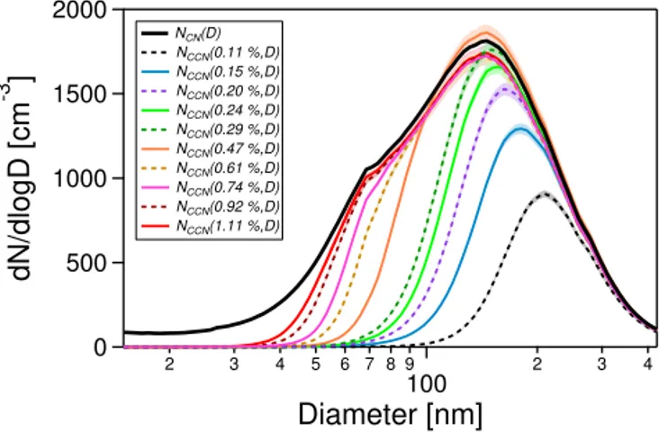
Figure 4 combines the annually averaged size distributions of NCN(D) as well as NCCN(S,D) for all S levels. These
curves result from multiplying theNCN(D) size distribution
with the CCN activation curves in Fig. 2 and clearly visu-alize the inverse relationship ofDa(S) andS. Following the
previous discussion of Fig. 2,S ranging between 0.11 and 0.29 % mostly activates accumulation-mode particles, while Sranging between 0.47 and 1.10 % activates the accumula-tion mode plus a substantial fracaccumula-tion of Aitken-mode parti-cles. For the highest supersaturation (S=1.10 %) that was used in this study, almost the entireNCN(D) size
2000
1500
1000
500
0
dN/dlogD [cm
-3 ]
2 3 4 5 6 7 8 9
100 2 3 4
Diameter [nm]
NCN(D)
NCCN(0.11 %,D)
NCCN(0.15 %,D)
NCCN(0.20 %,D)
NCCN(0.24 %,D)
NCCN(0.29 %,D)
NCCN(0.47 %,D)
NCCN(0.61 %,D)
NCCN(0.74 %,D)
NCCN(0.92 %,D)
NCCN(1.11 %,D)
Figure 4. Number size distributions of total aerosol particles,
NCN(D), and of cloud condensation nuclei,NCCN(S,D), at all 10 supersaturation levels (S=0.11–1.10 %) averaged over the entire measurement period. TheNCCN(S,D) size distributions were cal-culated by multiplying the average NCN(D) size distributions (in Fig. 3) with the average CCN activation curves in (Fig. 2).
sparse occurrence of particles<30 nm) explains the high NCCN(1.10 %)/NCN,10levels in Fig. 1d.
3.3 Seasonal differences in CCN properties at the ATTO site
Within the seasonal periods in the central Amazon as defined in Sect. 1.2, we have subdivided the annual data set into the following four periods of interest, which represent the con-trasting aerosol conditions and/or sources. (a) The first half of the wet seasons 2014 and 2015 received substantial amounts of long-range transport (LRT) aerosol: mostly African dust, biomass smoke, and fossil fuel emissions (Ansmann et al., 2009; Salvador et al., 2016). Here, the corresponding period of interest will be called LRT season and covers 24 March to 13 April 2014 and 9 January to 10 February 2015. (b) In the late wet season 2014, all pollution indicators approached background conditions. Thus, the period from 13 April to 31 May 2014 will be treated as the clean wet season in this study. (c) The months June to July represent the transition period from wet to dry season and will be called “transition wet to dry”. (d) The period of interest that covers the dry sea-son with frequent intrusion of biomass burning smoke ranges from August to December 2014.
Figure 5 shows the CCN activation curves for all S lev-els, subdivided into the four seasonal periods of interest. Al-though the plots for the individual seasons appear to differ only subtly, e.g., in Da(S) position and curve width, there is one major difference: the variable shape of the activa-tion curve for the smallest S=0.11 %. Particularly, the be-havior of MAF(0.11 %) shows clear seasonal differences. It reaches unity during the wet season, whereas it levels off below unity for the LRT, transition, and particularly for the
dry season periods. The fraction of non-activated particles withD≤245 nm atS=0.11 % is∼10 % during the tran-sition period and ∼20 % during the dry season. Interest-ingly, this effect is only observed forS=0.11 %, whereas MAF(>0.11 %) reaches unity throughout the entire year. An explanation for this observation could be the intrusion of relatively fresh biomass burning aerosol plumes during the transition period and dry season, which contain a fraction of comparatively inefficient CCN. Soot is probably a main candidate here; however, fresh soot should also significantly reduce the MAF(S) for higherS levels (Rose et al., 2010). Thus, we speculate that probably “semi-aged” soot particles may be an explanation for the observed activation behavior.
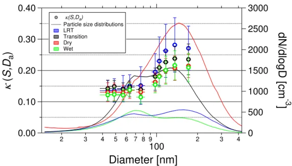
Figure 6 corresponds to Fig. 3 and subdivides the annual meanκ(S,Da)size distribution (κ(S,Da)plotted against all measuredDa(S)) as well as the annual meanNCN(D) size
distribution into their seasonal counterparts. The particle size distributions were fitted with a bimodal logarithmic normal distribution and the corresponding results are listed in de-tail in Table 2. The differences in the characteristic size dis-tributions for the individual seasons clearly emerge: in ad-dition to the strong variations in total particle number con-centration (see Fig. 1), the accumulation mode overwhelms the Aitken mode during the dry season, while accumulation and Aitken modes occur at comparable strength under wet season conditions. In other words, during the dry season, Aitken-mode particles account on average for about 26 % of the total aerosol population (NCN,Ait=483±49 cm−3
vs. NCN,Acc=1349±47 cm−3), whereas during the wet
season, the Aitken mode accounts for about 62 % (NCN,Ait=246±9 cm−3 vs. NCN,Acc=145±8 cm−3)(see
Table 2). The size distribution of the transition period from wet to dry season represents an intermediate state between the wet and dry season “extremes”. Furthermore, the com-parison between wet season conditions with and without LRT influence reveals comparable distributions. However, a slight increase in the accumulation mode during LRT conditions in-dicates the presence of dust, smoke, pollution, and aged sea spray on top of the biogenic aerosol population during pris-tine periods (M. L. Pöhlker et al., 2017a).
The Hoppel minimumDH (Hoppel et al., 1996) between
the Aitken and accumulation modes4 also shows seasonal variations with its largest values around 110 nm in the wet season and its smallest values around 95 nm in the dry sea-son (compare to Fig. 5 and Table 2). Following Krüger et al. (2014), the observed DH can be used to determine an
effective average cloud peak supersaturation Scloud(DH,κ).
4The position ofD
Figure 5.CCN activation curves for all measuredSlevels (S=0.11–1.10 %), subdivided into seasonal periods of interest as specified in Sect. 3.3. Data points represent arithmetic mean values. ForNCCN(S,D)/NCN(D), the standard error is plotted, which is very small (due to the large number of scans with comparatively small variability) and therefore not perceptible in this representation. For the diameter,
D, the error bars represent the experimental error as specified in Sect. 2.3. The grey vertical bands represent the (seasonal) position of the Hoppel minima (including error range; compare to Table 2). Dashed horizontal lines provide visual orientation and indicate 0, 50, and 100 % activation. The 50 % activation diameter is used for calculation of the hygroscopicity parameterκ(S,Da). The lines connecting the data points merely serve as visual orientation.
Cloud development and dynamics are highly complex pro-cesses in which aerosol particles are activated at different supersaturations. In the context of this study, Scloud(DH,κ)
is used as a mean cloud supersaturation and serves as an overall reference value; however, it does not reflect the com-plex development of S inside a cloud. Based on our data, Scloud(DH,κ) is estimated as a value around 0.29 % during
dry season conditions and around 0.22 % during wet season conditions (Table 2). This indicates thatScloud(DH,κ)levels
tend to be noticeable lower during wet season cloud devel-opment compared to the dry season scenario. A plausible cause for the comparatively smallDHand highScloud(DH,κ)
in the dry season could be invigorated updraft regimes in the convective clouds. This invigoration could be caused by the stronger solar heating during the dry season and/or the in-creased aerosol load under biomass-burning-impacted condi-tions, as suggested previously (Andreae et al., 2004; Rosen-feld et al., 2008). As outlined in Sect. 1.1, aerosol particle
size, concentration, and hygroscopicity as well as cloud su-persaturation represent key parameters for a detailed under-standing of cloud properties. Figure 6 provides reference val-ues for all these parameters, resolved by seasons and thus provides comprehensive insight into the Amazonian cloud properties.
Comparing the seasonal κ(S,Da) size distributions in Fig. 6, it is obvious that the (seasonally averaged)κAit
val-ues in the Aitken-mode size range are surprisingly stable be-tween 0.13 and 0.14 throughout the whole year. This indi-cates that the Aitken-mode aerosol population was persis-tently dominated by almost pure organic particles through-out the seasons. In contrast, noticeable seasonal differences were observed for (seasonally averaged)κAcc values in the
ingredi-3000
2500
2000
1500
1000
500
0
dN/dlogD [cm
-3
]
2 3 4 5 6 7 8 9
100
2 3 4Diameter [nm]
0.40
0.30
0.20
0.10
0.00
k
(
S,D
a
)
k(S,Da)
Particle size distributions LRT
Transition Dry Wet
Figure 6.Size dependence of the hygroscopicity parameterκ(S,Da)subdivided into seasonal periods of interest (color coding) as specified in Sect. 3.3. Values ofκ(S,Da)for everySlevel are plotted against their corresponding midpoint activation diameterDa(S) (left axis). For
κ(S,Da), the error bars represent 1 standard deviation. ForDa(S), the experimentally derived error is shown. In addition, the average number size distributions for the seasonal periods of interest are shown (right axis). The standard error of the number size distributions is indicated as shading, which is very small and therefore hardly perceptible in this representation due to the large number of scans with comparatively small variability. A clear size dependence and seasonal trends inκ(S,Da)levels can be observed. The averaged number size distributions show very pronounced seasonal differences.
ents (i.e., sulfate, ammonium, and potassium). In the size range around DH, which separates the (apparently)
chemi-cally distinct aerosol populations of Aitken and accumula-tion modes, a step-like increase inκ(S,Da)is observed. The highest seasonally averagedκ(S,Da)values (up to 0.28) are observed during intrusion of dust, marine sulfate, and sea-salt-rich LRT plumes. Note that short-term peaks inκ(S,Da) can be even higher; see case studies in Part 2 (M. L. Pöh-lker et al., 2017a). In the absence of LRT, the κAcc values
are also rather stable for most of the year and range between 0.21 and 0.24. Overall, a remarkable observation is the high similarity between the wet and dry seasonκ(S,Da)size dis-tributions, while many other aerosol parameters undergo sub-stantial seasonal variations (Andreae et al., 2015).
Theκ(S,Da)levels reported here agree well with the cor-responding results in the previous Amazonian CCN studies by Gunthe et al. (2009) and Whitehead et al. (2016), which range between 0.1 and 0.4, with a mean around 0.16±0.06. In a wider context, our results also agree well with previ-ous long-term measurements at other continental background locations (i.e., alpine, semi-arid, and boreal sites) (Jurányi et al., 2011; Levin et al., 2012; Paramonov et al., 2013; Mikhailov et al., 2015). Comparing these four sites with each other, the following observations can be made. (i)κAit
tends to be smaller than κAcc at all four background
loca-tions. (ii) At the alpine, semi-arid, and boreal sites,κ(S,Da) undergoes a rather gradual increase from the Aitken- to the accumulation-mode size range (Paramonov et al., 2013,
and references therein), whereas this increase appears to be steeper (step-like) in the Amazon. This can clearly be seen in the present study (e.g., Fig. 3) as well as in Gunthe et al. (2009) and Whitehead et al. (2016). (iii) Particularly in the vegetated environments (i.e., tropical, boreal, and semi-arid forests),κAitmostly ranges between 0.1 and 0.2,
sug-gesting that the Aitken-mode particles predominantly com-prise organic constituents. Furthermore,κAitshows a
remark-ably small seasonality for these locations. (iv) TheκAcclevels
show a much wider variability throughout the seasons for all locations.
Figure 7 presents the diurnal cycles inκmeanfor the four
seasonal periods of interest. No perceptible diurnal trends in κmeancan be observed for any of the seasons. The only
ob-servable difference is an increased variability ofκmean
dur-ing the LRT season (see error bars in Fig. 7a). This can be explained by the episodic character of LRT intrusions, which causes an “alternating pattern” of clean periods with back-ground conditions and periods of elevated concentrations of LRT aerosol (M. L. Pöhlker et al., 2017a). For comparison, the diurnal cycles inNCNconcentration have been added to
Figure 7.Diurnal cycles in hygroscopicity parameter,κmean, and total aerosol number concentration,NCN, subdivided into seasonal periods of interest as specified in Sect. 3.3. No diurnal trend is detectable throughout the year. Note that the range of 1 standard deviation of
κmeanaround the mean is surprisingly small given that long seasonal time periods and data from allSlevels have been averaged. The only perceptible difference is a larger scattering during a period with LRT influence(a). Grey and yellow shading indicate night and day.
3.4 Aerosol chemical composition and effective hygroscopicity
Continuous ACSM measurements are being conducted at the ATTO site since March 2014, providing online and non-size-resolved information on the chemical composition of the non-refractory aerosol (Andreae et al., 2015). Here, we compare the ACSM data on the aerosol’s chemical compo-sition with the CCNC-derivedκ(S,Da)values. This analysis focuses on the dry season months, when ACSM and CCNC were operated in parallel.5Note that the ACSM covers a size range from 75 to 650 nm (Ng et al., 2010), while the size-resolved CCN measurements provide information only up to particle sizes of about 170 nm. Since the ACSM records the size-integrated masses of defined chemical species (organics,
5Although the ACSM measurements were started in March 2014, instrumental issues during the initial months caused some uncertainty for the corresponding data. Thus, for this study, we focus only on the data period August to December 2014, when the instrumental issues were resolved.
nitrate, sulfate, ammonium, and chloride), the results tend to be dominated by the fraction of larger particles with com-paratively high masses (i.e., in the accumulation-mode size range) and are influenced less by the fraction of small parti-cles with comparatively low masses (i.e., in the Aitken-mode size range). Thus, in order to increase the comparability be-tween ACSM and CCNC, we have chosen the lowestSlevel (S=0.11±0.01 %), which represents the largest measured Da(S) (Da(S)=172±12 nm).
In Fig. 8, the κ(0.11 %,Da) values are plotted against the ACSM-derived organic mass fraction (forg). The data
were fitted with (i) a linear fit and (ii) a bivariate regres-sion according to Cantrell (2008). A linear fit approach was used by Gunthe et al. (2009) to determine the effec-tive hygroscopicity parametersκorg=0.1 of biogenic
Ama-zonian SOA (forg=1) andκinorg=0.6 for the inorganic
frac-tion (forg=0). For the present data set, the same
0.8
0.7
0.6
0.5
0.4
0.3
0.2
0.1
0.0
k
(
S,D
a
)
1.0 0.8 0.6 0.4 0.2 0.0
f
orgk(0.11 %,~170 nm) Bivariate regression:
m = -0.61 ± 0.01 b = 0.71 ± 0.01 R2 =0.71 Linear fit:
m = -0.49 ± 0.01 b = 0.61 ± 0.01 R2 =0.66
Figure 8.Correlation betweenκ(0.11 %,∼170 nm) and the organic mass fraction,forg, determined by the ACSM during the dry season months. The data were fitted by a linear and a bivariate regression fit. Shading of the fit lines shows the standard error of the fit. The er-ror bars of the data markers represent the experimental erer-ror, which is estimated as 5 % forforgand 10 % forκ(0.11 %,∼170 nm).
on the linear fit and extrapolation to forg=1 and forg=0,
respectively. This is in good agreement with previous studies (King et al., 2007; Engelhart et al., 2008; Gunthe et al., 2009; Rose et al., 2011). However, a drawback of the linear fitting approach is the fact that swappingforgandκ(0.11 %,Da)on the axes will change the results.
Therefore, we also applied the bivariate regression fit, which takes into account that both parameters, forg and
κ(0.11 %,Da), have an experimental error. For the bivariate regression, an error of 5 % in forg and an error of 10 % in
κ(0.11 %,Da)were used. A coefficient of determination of R2=0.71 was obtained for the bivariate regression, which is slightly better than for the linear fit. Based on the bivari-ate regression, we estimbivari-ated effective hygroscopicity param-eters κorg=0.10±0.01 andκinorg=0.71±0.01 for the
or-ganic and inoror-ganic fractions, respectively.
3.5 CCN parametrizations and prediction of CCN number concentrations
Cloud-resolving models at all scales – spanning from large eddy simulations (LESs) to global climate models (GCMs) – require simple and efficient parametrizations of the complex microphysical basis to adequately reflect the spatiotemporal CCN cycling (Cohard et al., 1998; Andreae, 2009). Previ-ously, several different approaches to predict CCN
concen-trations have been suggested (Andreae, 2009; Gunthe et al., 2009; Rose et al., 2010; Deng et al., 2013). Any parametriza-tion strategy seeks, on one hand, an efficient combinaparametriza-tion of a minimal set of input data and, on the other hand, a good representation of the atmospheric CCN population.
The detailed analysis in this study has shown that the CCN population in the central Amazon is mainly defined by com-paratively stable κ(S,Da) levels, due to the predominance of organic aerosol particles, and rather pronounced seasonal trends in aerosol number size distribution. Particularly, the remarkably stableκ(S,Da)values suggest that the Amazo-nian CCN cycling can be parametrized rather precisely for efficient prediction of CCN concentrations. In the follow-ing paragraphs, we apply the followfollow-ing CCN parametrization strategies to the present data set and explore their strengths and limitations:
i. CCN prediction based on the correlation be-tween NCCN(0.4 %) and NCN, called the
1NCCN(0.4 %)/1NCNparametrization here;
ii. CCN prediction based on the correla-tion between NCCN(S) and cCO, called the
1NCCN(S)/1cCOparametrization here;
iii. CCN prediction based on analytical fit functions of ex-perimentally obtained CCN spectra, called CCN spectra parametrization;
iv. CCN prediction based on theκ-Köhler model, called κ-Köhler parametrization; and
v. CCN prediction based on a novel and effective parametrization built on CCN efficiency spectra, called CCN efficiency spectra parametrization.
The prediction accuracy for the individual strategies is summarized in Table 3.
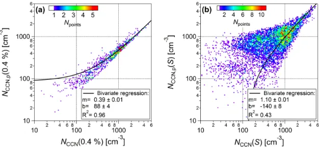
3.5.1 1NCCN(0.4 %)/1NCNparametrization
Andreae (2009) analyzed CCN data sets from several con-trasting field sites worldwide and found significant re-lationships between the satellite-retrieved aerosol optical thickness (AOT) and the corresponding NCCN(0.4 %)
lev-els as well as between the total aerosol number con-centration NCN and NCCN(0.4 %). The obtained ratio
NCCN(0.4 %)/NCN=0.36±0.14 – in other words, the
glob-ally averaged CCN efficiency atS=0.4 % – can be used to predict CCN concentrations. The corresponding results for the present data set are displayed in Fig. 9a and show a surprisingly tight correlation, given that a globally obtained NCCN(0.4 %)/NCN ratio has been used. However, Fig. 9a
also shows a systematic underestimation of the predicted CCN concentrationNCCN,p(0.4 %), which can be explained
T able 3. Characteristic de viation between observ ed and predicted CCN number concentrations – N CCN ( S ) and N CCN,p ( S ) – based on dif ferent parametrization schemes, ac-cording to Rose et al. (2008). F or ev ery parametrization scheme and resolv ed by S , the follo wing information is pro vided: (i) arithmetic mean v alues of the relati v e bias 1 bias N CCN ( S ) = ( N CCN,p ( S ) − N CCN ( S ))/N CCN ( S ) and (ii) of the total relati v e de viation 1 de v N CCN ( S ) = | N CCN,p ( S ) − N CCN ( S ) | /N CCN ( S ). S (%) 1N CCN (S )/1N CN 1N CCN (S )/1c CO Fits of CCN spectra κ -Köhler Erf fit of CCN ef ficienc y spectra T w ome y po wer -la w fit Erf fit Annual av erage Resolv ed by seasons annual seasonal annual seasonal bias de v bias de v bias de v bias de v bias de v bias de v bias de v bias de v bias de v bias de v bias de v 0.11 ± 0.01 – – 1.48 1.75 4.68 4.75 1.50 1.57 2.54 2.81 0.61 0.89 0.18 0.22 0.64 0.74 0.24 0.44 0.39 0.53 0.14 0.36 0.15 ± 0.02 – – 0.50 1.21 2.78 2.99 0.71 0.92 2.42 2.69 0.62 0.85 0.07 0.11 0.27 0.47 0.10 0.32 0.15 0.36 0.04 0.27 0.20 ± 0.02 – – 2.84 2.96 2.46 2.75 0.59 0.85 2.60 2.86 0.70 0.91 0.11 0.13 0.22 0.43 0.13 0.30 0.14 0.33 0.08 0.24 0.24 ± 0.03 – – 1.78 1.98 1.93 2.26 0.45 0.74 2.24 2.50 0.64 0.84 0.09 0.10 0.16 0.37 0.12 0.25 0.12 0.28 0.09 0.20 0.29 ± 0.03 – – 2.19 2.33 1.74 2.09 0.40 0.71 2.12 2.39 0.62 0.82 0.14 0.14 0.22 0.42 0.14 0.25 0.17 0.32 0.11 0.20 0.40 − 0.41 0.47 – – – – – – – – – – – – – – – – – – – – 0.47 ± 0.04 – – 1.33 1.54 1.36 1.73 0.33 0.63 1.70 1.93 0.50 0.71 0.04 0.06 0.09 0.26 0.07 0.16 0.08 0.20 0.06 0.12 0.61 ± 0.06 – – 1.02 1.15 1.23 1.55 0.36 0.61 1.47 1.73 0.47 0.67 0.08 0.09 0.08 0.18 0.05 0.09 0.08 0.15 0.05 0.08 0.74 ± 0.08 – – 1.50 1.59 1.22 1.51 0.40 0.62 1.37 1.63 0.44 0.64 0.09 0.10 0.09 0.16 0.04 0.06 0.09 0.14 0.04 0.06 0.92 ± 0.11 – – 1.11 1.28 1.15 1.42 0.45 0.63 1.18 1.44 0.40 0.60 0.08 0.08 0.05 0.10 0.01 0.03 0.05 0.09 0.01 0.04 1.10 ± 0.08 – – 1.12 1.25 1.11 1.35 0.48 0.64 1.05 1.31 0.35 0.57 0.08 0.08 0.04 0.08 − 0.01 0.04 0.05 0.08 − 0.01 0.05 All – – 1.50 1.73 2.00 2.27 0.57 0.80 1.89 2.15 0.54 0.75 0.10 0.11 0.19 0.33 0.10 0.20 0.14 0.25 0.06 0.17
see Fig. 1). Activated fractions in other locations worldwide tend to be lower due to the (more persistent) abundance of nucleation-mode particles, as discussed in Sect. 3.1.
In Sect. 3.5.5, we will show that our novel parametrization is an extension of this approach: the NCCN(0.4 %)/NCN parametrization refers to a globally
averaged CCN efficiency at one specificS, while the CCN efficiency spectra parametrization is based on an analytical description of CCN efficiencies across the entire (relevant) Srange and has been determined specifically for the central Amazon.
3.5.2 1NCCN(S)/1cCOparametrization
Experimentally obtained excess NCCN(S) to excess cCO
ratios can be used to calculateNCCN,p(S). Kuhn et al. (2010)
determined 1NCCN(0.6 %)/1cCO= ∼26 cm−3ppb−1 for
biomass burning plumes and 1NCCN(0.6 %)/1cCO= ∼49 cm−3ppb−1 for urban emissions in the area around Manaus, Brazil. Lawson et al. (2015) investi-gated biomass burning emissions in Australia and found 1NCCN(0.5 %)/1cCO=9.4 cm−3ppb−1. In the context of
the present study, we have calculated1NCCN(S)/1cCO for
a strong biomass burning event in August 2014. This event and its impact on the CCN population is the subject of a detailed discussion in the companion Part 2 paper (M. L. Pöhlker et al., 2017a). Here, we use the1NCCN(S)/1cCO
ratios from the companion paper to obtain a CCN pre-diction. The observed 1NCCN(S)/1cCO ratios range
between 6.7±0.5 cm−3ppb−1 (for S=0.11 %) and values
around 18.0± 1.3 cm−3ppb−1(for higherS) (see summary
in Table 4). Since biomass burning is the dominant source of pollution in the central Amazon, these biomass-burning-related 1NCCN(S)/1cCO ratios in Table 4 were used to
calculate NCCN,p(S) for the present data set. The
corre-sponding results in Fig. 9b show a reasonable correlation for highly polluted conditions (NCN>2000 cm−3) and a
poor correlation for cleaner states (NCN<2000 cm−3).
This behavior can be explained by the fact that the high concentrations in CCN and CO originate from frequent biomass burning plumes during the Amazonian dry season (see Fig. 1). Thus, they can be assigned to the same sources with rather defined1NCCN(S)/1cCOratios (Andreae et al.,
2012). During the contrasting cleaner periods, CN and CO originate from a variety of different sources, which are often not related and therefore explain the poor correlation for clean to semi-polluted conditions. Overall, Fig. 9b indicates that the quality of CO-based CCN prediction is rather poor, due to the complex interplay of different sources. The overall deviation betweenNCCN,p(S) andNCCN(S) for this approach
Figure 9. Predicted vs. measured CCN number concentrations calculated from (a) observed ratio NCCN(0.4 %)/NCN=0.36 in An-dreae (2009) and(b)observed (biomass-burning-related) excess CCN to excess CO ratios in M. L. Pöhlker et al. (2017a). The color code shows the number of data points falling into the pixel area, following Jurányi et al. (2011). The black line represents a bivariate regression fit of the data.
Table 4.ExcessNCCN(S) to excesscCO ratios1NCCN(S)/1cCOfor the individualS levels during peak period of the strong biomass burning event in August 2014. This event is analyzed in detail through a case study in the companion Part 2 paper (M. L. Pöhlker et al., 2017a). The values1NCCN(S)/1cCOwere obtained from bivariate regression fit of scatterplots betweenNCCN(S) andcCOfor individual Slevels (Andreae et al., 2012). The parameterNCCN(S)in this table represents theyaxis intercept of the linear regression ofNCCNvs.cCO
atcCO=0 ppb and is, therefore, negative (see M. L. Pöhlker et al., 2017a).
S(%) 1NCCN(S)/1cCO(cm−3ppb−1) NCCN(S)(cm−3) R2 0.11±0.01 6.7±0.5 −603±125 0.86 0.15±0.02 13.6±1.4 −1447±354 0.68 0.20±0.02 14.3±0.8 −1128±208 0.90 0.24±0.03 16.8±1.0 −1460±261 0.86 0.29±0.03 17.4±1.3 −1378±296 0.83 0.47±0.04 20.1±1.7 −1675±425 0.84 0.61±0.06 17.9±1.3 −1206±332 0.88 0.74±0.08 16.5±1.3 −933±329 0.88 0.92±0.11 18.1±1.4 −1265±355 0.85 1.10±0.08 17.5±1.3 −1096±328 0.87
3.5.3 Classical and improved CCN spectra parametrization
The total number of particles that are activated at a given S is regarded as one of the central parameters in cloud for-mation and evolution (Andreae and Rosenfeld, 2008). Thus, CCN spectra (NCCN(S) plotted againstS) are a widely and
frequently used representation in various studies to summa-rize the observedNCCN(S) values over the cloud-relevantS
range for a given time period and location (Twomey and Wo-jciechowski, 1969; Roberts et al., 2002; Rissler et al., 2004; Freud et al., 2008; Gunthe et al., 2009; Martins et al., 2009b). Different analytical fit functions of the experimental CCN spectra have been proposed and are used as parametrization schemes for NCCN(S) in modeling studies (e.g., Cohard et
al., 1998; Khain et al., 2000; Pinsky et al., 2012; Deng et al., 2013).
In the context of the present study, the annual mean Ama-zonian CCN spectrum is shown in Fig. 10. As an analyti-cal representation of the experimental data, we have used Twomey’s empirically found (classical) power-law fit func-tion (Twomey, 1959):
NCCN(S)=NCCN(1 %)·
S
1 %
k
, (6)