www.atmos-chem-phys.net/10/10161/2010/ doi:10.5194/acp-10-10161-2010
© Author(s) 2010. CC Attribution 3.0 License.
Chemistry
and Physics
New trajectory-driven aerosol and chemical process model
Chemical and Aerosol Lagrangian Model (CALM)
P. Tunved1, D. G. Partridge1, and H. Korhonen2
1Department of Applied Environmental Science Stockholm University, 106 91, Stockholm, Sweden 2Finnish Meteorological Institute, Kuopio Unit, P.O. Box 1627, 70211 Kuopio, Finland
Received: 24 May 2010 – Published in Atmos. Chem. Phys. Discuss.: 21 June 2010
Revised: 28 September 2010 – Accepted: 28 September 2010 – Published: 1 November 2010
Abstract. A new Chemical and Aerosol Lagrangian Model (CALM) has been developed and tested. The model incor-porates all central aerosol dynamical processes, from nucle-ation, condensnucle-ation, coagulation and deposition to cloud for-mation and in-cloud processing. The model is tested and evaluated against observations performed at the SMEAR II station located at Hyyti¨al¨a (61◦51′N, 24◦17′E) over a time period of two years, 2000–2001. The model shows good agreement with measurements throughout most of the year, but fails in reproducing the aerosol properties during the win-ter season, resulting in poor agreement between model and measurements especially during December–January. Never-theless, through the rest of the year both trends and magni-tude of modal concentrations show good agreement with ob-servation, as do the monthly average size distribution prop-erties. The model is also shown to capture individual cleation events to a certain degree. This indicates that nu-cleation largely is controlled by the availability of nucleat-ing material (as prescribed by the [H2SO4]), availability of condensing material (in this model 15% of primary reactions of monoterpenes (MT) are assumed to produce low volatile species) and the properties of the size distribution (more specifically, the condensation sink). This is further demon-strated by the fact that the model captures the annual trend in nuclei mode concentration. The model is also used, along-side sensitivity tests, to examine which processes dominate the aerosol size distribution physical properties. It is shown, in agreement with previous studies, that nucleation governs the number concentration during transport from clean areas. It is also shown that primary number emissions almost ex-clusively govern the CN concentration when air from Cen-tral Europe is advected north over Scandinavia. We also show that biogenic emissions have a large influence on the
Correspondence to:P. Tunved ([email protected])
amount of potential CCN observed over the boreal region, as shown by the agreement between observations and modeled results for the receptor SMEAR II, Hyyti¨al¨a, during the stud-ied period.
1 Introduction
The representation of particles in the atmosphere remains one of the largest uncertainties in predicting our future cli-mate (IPCC, 2007). Knowledge of the particle abundance, chemistry and size is of crucial importance to determine both indirect and direct climate effects of particles in the atmo-sphere. In order to accurately describe the aerosol properties on large spatial scales, more efficient ways to parameterize important aerosol processes are needed. While regional and global transport models incorporating aerosol schemes are quite numerous, they often include quite coarse parameteri-zations of the dynamical processes relating to aerosols in the atmosphere. Typically, this is due to computational limita-tions.
In this study we present a new box model framework adopting state of the art aerosol dynamic description that will aid in the understanding of the different processes affecting the aerosol over the boreal regions, and in the future also at other sites. The model is a two layer box model that is in-tended to run along trajectories.
The aim with the study is to test this trajectory driven La-grangian process model that seeks to capture and describe the processes that govern the evolution of aerosol chem-ical and physchem-ical properties. In this study we have fo-cused on the processes dominating the aerosol as observed at Hyyti¨al¨a SMEAR station, Southern Finland (61◦51′N, 24◦17′E, 181 m a.s.l.). The SMEAR station has the longest record of aerosol number size distribution observations, dat-ing back to 1996, and also facilitates numerous measure-ments of other aerosol parameters and trace gases. The sur-roundings are dominated by a flora mainly consisting of pine forests of an age of roughly forty years. The closest large city is the city of Tampere some 60 km away from the station. The location of Hyyti¨al¨a, in the southern rim of the Scan-dinavian boreal region, makes it an excellent site to study both the role of anthropogenic as well as natural emissions. The location allows studies of natural sources when the air masses originating from the marine environment transport over the forest, as well as of aged anthropogenic air down-stream of the large pollution sources in continental Europe. This fact has been demonstrated in a number of studies, and northerly and southerly transport of air is associated with distinct features. As has been shown in previous studies, marine air transport over the forested regions is associated with a rapid increase in aerosol number and, to a somewhat smaller extent, in mass (e.g. Tunved et al., 2006a, b). This increase in number appears to be controlled by nucleation mediated by sulfuric acid while the growth mainly seems to be facilitated by organics originating from the forest it-self, most likely monoterpenes (MT) or similar compounds (e.g., Tunved et al., 2006a; Laaksonen et al., 2008). How-ever, when polluted air arrives from the south it is seen that nucleation is largely absent over the forest, and number con-centrations typically decrease when transport further north-wards takes place (Tunved et al., 2005). Although located far from major pollution sources, observations at Hyyti¨al¨a do show that continental influence may occasionally domi-nate the aerosol properties (Dal Maso et al., 2007; Tunved et al., 2003) providing the site with a fairly large concentration of accumulation mode-sized particles.
In this study we use the newly developed model CALM to study the integrated effect of both natural and anthropogenic sources, as well as primary and secondary aerosol produc-tion. Using a number of sensitivity tests, we identify the pro-cesses dominating the appearance and abundance of particles associated with air-masses of different origin. The difference between e.g. marine and continental air sources will be dis-cussed in terms of the role of primary and secondary emis-sions. Several other model studies have been performed at
Hyyti¨al¨a, covering a wide range of complexity (Eulerian pro-cess studies, Lagrangian propro-cess studies, Tunved et al., 2004, global model studies, Spracklen et al., 2006). Aside from the general features of the aerosol, many of these studies have focused on the role and mechanisms of nucleation over the forest and on the importance of primary emissions.
2 General model design
The basic model design consists of a trajectory driven box model. The model is fed with back trajectories along which the process model simulates the evolution of both aerosol and gas species. The current model setup adopts a two layer structure, a residual and mixing layer (RL and ML, respec-tively). Both compartments are assumed to be well mixed internally. The trajectory dictates the transport of the model space described by these internally well mixed boxes. The trajectory itself however is not assigned specifically to ei-ther of the boxes, but instead describes the movement of this simplified model system along the geographical coordinates of the trajectory. Exchange between the layers is allowed, and this exchange is governed by the variation of the mixing layer height (MLH). The MLH typically follows a diurnal cycle with a maximum around noon. The MLH is calcu-lated by the HYSPLIT4 model along the trajectories and is defined as the height level at which the potential temperature is at least two degrees greater than the minimum potential temperature. During morning hours, when the mixing layer starts to grow into the residual layer, the mixing layer gases and aerosols are mixed with their counterparts in the resid-ual layer, a process that most of the time leads to dilution of the ML quantities. When the MLH starts to decrease, the ML aerosol and gases get partially trapped within the resid-ual layer. The height of the mixing layer is provided by the trajectory model and typically varies between 250 m (which is the lower limit from the trajectory model) and some thou-sand meters above the ground level. Throughout each sim-ulation the residual layer upper limit remains constant. This upper boundary of the model compartment is defined as the maximum MLH of each simulated trajectory and typically reaches altitudes around 1500–2500 m. There are no inter-actions with the air above the modeled layers in the current set-up.
emissions from water surfaces. Other relevant meteorolog-ical parameters, such as relative humidity and ML height, were extracted from trajectory calculations as well.
In both layers we allow for general aerosol dynamics (e.g. condensation, nucleation, coagulation) as well as pho-tochemistry. However, deposition is only considered in the ML and all ground based emissions are initially confined to the ML, although may be transported into the RL due to vari-ation of the MLH. Two types of clouds are considered: stra-tus type and cumulus type clouds. The model setup only al-lows for clouds in the mixing layer. The frequency of clouds is described using available statistics of cloudiness over the model domain. Precipitation scavenging is accounted for in both ML and RL. The treatment of these processes will be described in detail below.
2.1 Aerosol dynamic model
The aerosol particle dynamics is described using the Univer-sity of Helsinki Multicomponent Aerosol model (UHMA) described in detail by (Korhonen, Lehtinen and Kulmala, 2004). The model incorporates the major microphysical processes that affect the aerosol under clear sky conditions, namely nucleation, coagulation, multi-component condensa-tion and dry deposicondensa-tion. In the current model setup we as-sume that the aerosol is distributed over 45 log-normally dis-tributed bins over the size range 0.2 nm–1.2 µm. The parti-cles are assumed internally mixed in every size bin. In each bin we allow a composition defined by three different compo-nents: sulfuric acid, soluble organics and insoluble species. In the setup we assume that component one represents sul-fur and sea salt, component two represents both primary and secondary formed organic aerosol constituents and compo-nent three represents insoluble species (i.e. soot in the current setup).
Nucleation is represented by the activation theory, where the nucleation rate is directly proportional to the concentra-tion of sulfuric acid, [H2SO4], with an empirically defined correlation coefficient,A(Kulmala, Lehtinen and Laaksonen 2006). The value ofAhas been set to 2×10⁻⁶following em-pirical findings at Hyyti¨al¨a (Riipinen et al., 2007). It is worth mentioning thatAvaries between different locations and sea-sons, reflecting the other unknown components necessary to accurately describe the rate of nucleation. ThusAmay be described as an environment-specific constant, but since the information available on the value ofAis still somewhat lim-ited we assume thatAremains constant through the simula-tions. As we will see, this will not substantially affect the final simulated size distribution at the receptor location.
The dry deposition for particles and gases is calculated for the 17 classes of land cover in the International Geosphere-Biosphere Programme (IGBP; Loveland and Belward, 1997) global vegetation classification scheme. The Land Cover Classification product (MOD12Q1) includes 11 natural
veg-etation classes, 3 developed land classes (one of which is a mosaic with natural vegetation), permanent snow or ice, bar-ren or sparsely vegetated land, and water.
Dry deposition is calculated following the dry deposition procedure by the EMEP/MSC-E regional model of heavy metals airborne pollution (MSCE-HM), using variations on the resistance analogy approach (Wesely et al., 1989) for each surface type (as documented by Travnikov and Ilyin, 2005).
The dry deposition of gases is calculated following the gaseous deposition model by Zhang et al. (2003). This model utilizes a “big-leaf” resistance approach model for represent-ing the process of gaseous deposition. It is very important to describe in some manner the deposition of terpenes within CALM. It is difficult to assign the gas properties, e.g. molec-ular diffusivities, for these organic compounds since there are very few measurements in the literature. Therefore for con-sistency the carbonyl groups presented by Zhang et al., 2003 are used as a proxy for these gases in CALM.
2.2 Chemical model
The gas-phase chemistry is solved using the quasi-stationary state assumption (QSSA). The chemistry module solves the chemistry for every time step of the simulation, thereby up-dating the concentration of the included species. Besides chemical reactions, the trace constituents are also subject to deposition (wet and dry) and removal from the gas phase via condensation onto existing particles (and naturally also nu-cleation, as in the case for sulfuric acid, see Sect. 2.2). In this study we estimate the chemistry for 76 different compounds and intermediates. The module solves the chemistry of the most important oxidants; hydroxyl radicals (OH, HO2), ni-trate radicals (NO3)and ozone (O3).
constants are adjusted accordingly, assuming a cloud optical depth of 20 (corresponding to reasonable cloudiness), mod-ifying photolysis constants above (i.e. in the residual layer) and below the cloud column (i.e. in the mixing layer).
The terpene chemistry is represented by the relatively well-known reaction chain of α-pinene, and the reaction scheme used is the one presented in (Andersson-Skold and Simpson 2001)and references therein. This reaction scheme includes the reactions ofα-pinene and its products consider-ing oxidative reactions includconsider-ing nitrate radicals (NO3), hy-droxyl radicals (OH) and ozone (O3). While the reactions described in this scheme certainly are important for the gas phase chemistry, e.g. radical abundance and ozone produc-tion, we do not use the products in this scheme explicitly when estimating the production of condensable species. In-stead, we assume a fixed stochiometric yield of 15% con-densable compounds from the primary reactions betweenα -pinene and NO3, OH and O3. This compound is assumed to have saturation vapor pressure of 3×10¹²molecules per cu-bic meter, and molar mass of 186 g mol−1(Kulmala, Laakso-nen and Pirjola, 1998). The yield agrees well with earlier es-timates presented by Tunved et al. (2006b) (using 13%) con-sidering what is required to reproduce the observed growth rates of particles over the boreal forest.
Isoprene chemistry follows the scheme suggested by Simpson et al. (EMEP, MSC-W, 1993), including 18 differ-ent reactions of isoprene and its products.
Sesquiterpenes are assumed to be immediately oxidized once emitted, and thus we do not describe their chemistry at all. Sesquiterpenes are highly reactive, and are quickly oxidized under atmospheric conditions. Chamber studies in-dicate that the aerosol mass yield from its oxidation by com-mon oxidants is between 17–67% (Griffin et al., 1999). In our setup 20% of the emitted sesquiterpenes are assumed to form a condensable product with the same properties as that formed from mono-terpene oxidation.
In the current setup, ethane is assumed to represent all an-thropogenic NMVOC emissions. The chemistry of ethane is described using the reaction sequence presented by Simp-son et al. (EMEP, MSC-W, 1993). The same goes for the methane chemistry.
With the reactions outlined above, the chemistry of NOx is solved and the ozone HOx(OH, HO2) and nitrate radical concentrations are calculated.
2.3 Cloud description
The occurrence of clouds is prescribed randomly in the model. The cloud frequency, however, is constrained by ob-servational seasonal data. The cloud frequency for differ-ent seasons and locations (Dec–Feb, Mar–May, Jun–Aug, Sep–Nov) are adopted from the online Climatic Atlas of Clouds over Land and Ocean (http://www.atmos.washington. edu/∼ignatius/CloudMap/, Warren et al., 2006). This
ap-proach allows for both seasonal and spatial constraints with
respect to cloud frequency over the simulated domain. The cloud types considered are stratus type clouds and cumulus type clouds. The stratus type clouds fill the upper 150 m of the ML. The typical coverage of the stratus clouds is set to 6/8. The cumulus type clouds are assumed to form from the middle of the mixing layer up to the top of the mixing layer. Furthermore cumulus clouds are only present when the mix-ing layer height is above 600 m. The typical coverage of the cumulus type clouds is set to 4/8 or 50%. This means that only a fraction of the aerosol will be processed by a cloud, and this fraction is based on the horizontal coverage and ver-tical extent of the cloud as described above.
When a cloud is assumed to form, the ML aerosol size distribution and associated properties are fed to the cloud module, where the dynamics of the aerosol population in the clouds is described using the common growth equations (e.g. Seinfeld and Pandis, 1998), using a constant updraft through the cloud. The updraft in turn depends on the cloud type. Stratus type clouds are allowed to have a prescribed updraft between 0.025–0.125 ms−1and the cumulus type clouds are allowed to have an updraft between 1–3 ms−1. Although fixed for the individual clouds simulated, the updraft for ev-ery cloud cycle is determined randomly, allowing the up-draft to vary within the above-mentioned limits from case to case. The growth is calculated based on the size and com-position of the aerosol particles. Sulfates are assumed to be completely soluble, while the solubility of the organics is as-sumed to be 10%. Variable aerosol properties (such as size and chemistry) and variable updraft will thus govern a varia-tion in lowest activavaria-tion radius from case to case. The droplet growth in the cloud is described using the moving center ap-proach, in contrast to the fixed sectional approach adopted for the “dry” aerosol dynamics.
The current setup of clouds allows for no precipitation, and thus no in-cloud scavenging. This is admittedly a com-promise. Several attempts were made to mimic the in-cloud scavenging by allowing the shallow in-clouds to precip-itate. However, the results soon became unrealistic since the aerosol was removed too quickly from the modeled two layer column. Thus, it was concluded that the current setup could not provide realistic precipitation description. Instead, precipitation data (mm h−1)are taken from the HYSPLIT4 model output. This precipitation is assumed to fall through both the RL and ML, but the precipitating cloud itself is formed above the modeled column. In practice, this means that explicit treatment of in-cloud scavenging is omitted in the model since the cloud is formed on an aerosol outside the modeled column. This approach is likely valid for frontal type precipitation (i.e. nimbostratus) considering that (1) the front itself serves as a boundary between two air-masses and (2) the air flows behind and ahead of the front are not the same since they occur in different air-masses. In practice, the movement of a warm front includes lifting of the warm air on top of the colder air-mass. Since the trajectories are calculated arriving at 100 m and given the fact that the tra-jectories rather seldom subside close to the station, the like-lihood for a trajectory having spent time inside a NB-type cloud during the last couple of days is typically small. This means that rainout processes (i.e. in-cloud scavenging) are less likely to affect the mixing layer aerosol as compared to washout processes (i.e. below cloud scavenging) consider-ing timescales of a couple of days. Thus, in the model we assume washout (i.e. below cloud scavenging) of aerosols only. For this purpose we make use of the parameterization presented by (Laakso et al., 2003). This empirically derived parameterization is based on 6 years of ground level size dis-tribution data measured at Hyyti¨al¨a (61◦51′N, 24◦17′E) and
provides size dependent scavenging coefficients between 10– 500 nm. In this study, the parameterization is extrapolated up to 1 µm. Since the approach of the study presented by Laakso et al., incorporates size distribution data and precip-itation data measured on the ground level, the resulting pa-rameterization will largely describe below cloud scavenging, but since the approach relies on the measured rate of change in aerosol concentration versus precipitation intensity, also other processes will by necessity affect the rate of change in aerosol properties (i.e. size dependent number concentra-tion). This means that the parameterization will also indi-rectly take into account in-cloud scavenging if the precipi-tation takes place in a cloud confined within a well mixed boundary layer.
The CALM cloud module further takes into account in-cloud oxidation of sulfate by ozone and hydrogen peroxide. We here use a bulk-water approach by summing up the total volume of water in the cloud. The bulk-water of the cloud is assumed to be infinitely dilute and is iteratively equili-brated to the surrounding gases (NH3, SO2,H2O2, O3, CO2) and pH is evaluated based on the amount of dissolved gases
and aerosol bulk composition (considering the sulfate frac-tion only). The soluble gases (SO2, NH3, O3and H2O2)are partitioned between gas and liquid phase based on thermo-dynamical limitations. The in-cloud oxidation of S(IV) to S(VI) is initialised by calculating the pH of the cloud bulk water, taking into account the liquid water content (LWC), concentration of surrounding gases and the particle content of sulfate. Once the pH has been established and the equi-librium of reacting gases has been reached, the liquid phase oxidation is calculated. The pH and concentration of reacting gases in the liquid phase are recalculated every time step.
d[S(IV)O3]/dt= [O3,aq](k0[H2SO3] +k1[HSO3−] +k2[SO32−])(R1)
d[S(IV)H2O2]/dt=k4[H3O+][HSO3−][H2O2,aq]/(1+K[H3O+)(R2)
Reaction constants used are those from Seinfeld and Pan-dis (1998). When the cloud Pan-dissipates, the produced sul-fate (equivalent amount of sulfuric acid) is distributed over the size range of activated particles following the sectional method. Each particle gains sulfate proportional to the in-dividual water content of the droplet. This causes activated particles to leave the cloud with a larger size than they en-tered the cloud, and clouds thus provide a source of sulfate in the model.
The gas phase chemistry if further indirectly affected by cloudiness. When clouds are present, the photolysis con-stants are adjusted accordingly, assuming a cloud optical depth of 20 (corresponding to reasonable cloudiness), mod-ifying photolysis constants above (i.e. in the residual layer) and below the cloud column (i.e. in the mixing layer). 2.4 Emissions
2.4.1 BVOC
In the model setup we consider biogenic emissions from dif-ferent land use types according to the IGBP land use maps (Loveland and Belward 1997): needle leaf forest, mixed for-est, deciduous needle leaf forfor-est, open shrubs, closed shrubs, grasslands, permanent wetlands and croplands. The land use type is defined as a fraction per grid of the land use map (0–1 on a quarter degree grid). To apply a seasonal dependence on the foliar biomass density we adopt the Global Inventory Modeling and Mapping Studies (GIMMS) Normalized Dif-ference Vegetation Index (NDVI, Tucker et al., 2004), from which we derive a foliar biomass density using the equations as presented in (Guenther et al., 1995)and references therein. The NDVI data is used as follows:
The monthly average of the Global vegetative indices (G) is calculated as:
G=100(1+NDVI) (1)
And the foliar biomassDmdensity is calculated as:
Dprepresents annual peak foliar density.Dmis only
cal-culated ifGis above a certain thresholdG2. Representative values ofG2are taken from (Guenther et al., 1995). Other-wise,Dmis set to zero.Dpis in turn calculated as
Dp=Dr×NPP (3)
WhereDr is an empirical coefficient and NPP represent
the net primary production taken from tabulated values for different ecosystem types corresponding to our IGBP land use classification.
The emission potential for spruce and pine is allowed to vary depending on season (Tarvainen et al., 2007). For de-ciduous forests we assume an emission potential of monoter-penes of µg g (dry weight)−1h−1(i.e. emissions per hour and gram of leaf dry weight).
Biogenic Volatile Organic Compounds (BVOC) are as-sumed to consist of monoterpenes (represented byα-pinene), isoprene and sesquiterpenes. Concerning the mono- and sesquiterpenes emissions we assume pool dependent tem-perature controlled emissions (Guenther et al., 1993, 1995). Monoterpene emissions are strongly dependent on temper-ature and the total flux of terpenes can be calculated us-ing the relationF=εDγ, whereF represent the total flux of monoterpenes from the forest in µg m−2h−1, ε is the emission potential (µg g (dry weight)−1h−1), D is the fo-liar biomass density in g (dry weight) m−2, andγ is an en-vironmental correction taking into account the temperature dependency of the emission rate (γ(pool) = exp(β(T−Ts)),
β= 0.09 C−1 and Ts= 303.15).The temperature used is the
surface temperature as derived from the FNL data set used for trajectory calculations. The sesquiterpenes are calcu-lated in a similar manner, but with a seasonal dependence of the emission potential associated with conifer trees with a zero emission potential through November-March (Hakola et al., 2006). No light dependence is considered for monoter-pene emissions. Isoprene is calculated following Guenther et al. (1995). This isoprene emission estimates adopts both light and temperature dependence. The photosynthetic pho-ton flux density (PPFD) is calculated following (Alados-Arboledas et al., 2000). The clear sky values of the PPFD are used regardless of cloudiness in the model. The emission potentials used are 0.1 µg g (dry weight)−1h−1 for conifers and 1 µg g(dry weight)−1h−1for deciduous trees.
2.4.2 Other trace gases
In its current form, the model allows for gridded emis-sions of the most common inorganic trace gases as well as anthropogenic emissions of non-methane volatile organic compounds (NMVOC). These emissions are taken from the EMEP data base (50×50 km grid, Vestreng et al., 2006) and include besides NMVOC (in our study represented by ethane) also CO, anthropogenic SO2, natural SO2,and NO.
The emissions are adjusted to comply with the seasonal emis-sion pattern (D. Simpson, personal communication, 2007).
DMS emissions are calculated according to (Kettle et al., 1999), making use of monthly mean sea surface DMS con-centrations. Actual DMS fluxes are calculated from these surface water concentrations by using surface temperature and wind speed.
2.4.3 Primary emissions
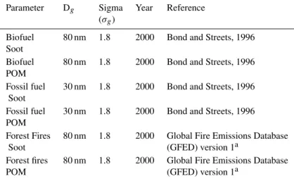
The model also incorporates primary aerosol emissions. For this purpose, the model includes anthropogenic emissions of anthropogenic primary organic particles (POA) as well as POA emissions from forest fires. These emissions are taken from the AEROCOM database (Dentener et al., 2006)using year 2000 as reference. The emissions are mass based, but remapped to standard size distributions as shown in Table 1. The seasonal dependence for the emissions is accounted for by applying the previously discussed seasonal scaling factors also for these data sets. The forest fire emissions are however given as monthly values throughout the year. Sea spray emis-sions are estimated assuming dependence on wind speed and temperature following (Martensson et al., 2003).
3 Results
In the following the general model performance will be dis-cussed followed by an investigation of the model’s sensitiv-ity to certain key processes/parameters. The model is initial-ized with either a marine, rural or polluted continental size distribution, depending on the starting location. The model parameters of these initial size distributions are given in Ta-ble 2. The model is further initialized, regardless of start-ing location and/or time of year with 35 ppb ozone, 40 ppt SO2and 500 ppt NOx. CO is a rather long lived species and also plays an important role in regulating the abundance of oxidants in the atmosphere. Therefore, initial CO concen-trations are selected based on both season and location, i.e. either summer or winter values for continental and marine starting locations (100 and 220 ppb for summer and winter time continental locations and 100 and 150 ppb for summer and winter marine locations, thereby adopting typical values to initialize the model). All BVOC are initially set to zero. Methane is set to 1750 ppb.
3.1 A single trajectory run: simplified description of processes
In order to show the evolution of some selected key param-eters along a trajectory run we selected a case where marine air is advected over Scandinavia (Fig. 1). Time and date of this simulation ends at 13 April 2000, 06:00 UTC. The model was simulated along the trajectory shown in Fig. 1 for 216 h, i.e. 9 days, starting in the marine Arctic environment. The evolution of selected parameters is displayed in Fig. 2, where the concentration of SO2, O3, H2SO4, (condensable
Table 1.Adopted size distribution properties of the various AEROCOM primary emissions. Shown is the sigma and geometric mean for the emission size distribution and emission year used for each sector.
Parameter Dg Sigma Year Reference
(σg)
Biofuel 80 nm 1.8 2000 Bond and Streets, 1996 Soot
Biofuel 80 nm 1.8 2000 Bond and Streets, 1996 POM
Fossil fuel 30 nm 1.8 2000 Bond and Streets, 1996 Soot
Fossil fuel 30 nm 1.8 2000 Bond and Streets, 1996 POM
Forest Fires 80 nm 1.8 2000 Global Fire Emissions Database
Soot (GFED) version 1a
Forest fires 80 nm 1.8 2000 Global Fire Emissions Database
POM (GFED) version 1a
ahttp://ess1.ess.uci.edu/∼jranders/data/GFED2/
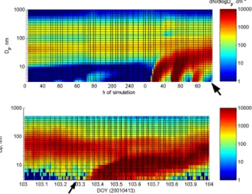
is accompanied by Fig. 3 showing the evolution of aerosol number size distribution along the trajectory (top frame) as well as the observed evolution of the aerosol number size distribution as observed at Hyyti¨al¨a during the final day of the simulation (lower frame). As can be seen from the fig-ures, as long as the air resides over the marine environment, some nucleation is taking place, but the magnitude of both nucleation and growth is too low to support production of particles that will be stable for a longer period of time. How-ever, as soon as the air arrives at the coast, the onset of bio-genic emissions (represented by MT, third panel in Fig. 2) provides the amount of organic gases to support the growth. The air parcel reaches the coast after approximately 144 h of simulation, and during the following days, three consecutive nucleation events are suggested by the model, of which each one is contributing to increasing number concentration. The simulated day is also associated with nucleation at the recep-tor site Hyyti¨al¨a which is evident from Fig. 3 (lower frame), a typical feature observed at this station when marine polar and arctic air masses arrive at the station. The idea that the forest supports the growth has been pointed out in numerous studies as discussed in the introduction and the current model result suggests that several consecutive, nucleation events provide the number concentration that is observed at the station when this type of transport takes place. As a comparison, the re-sulting simulated and observed aerosol number and volume size distributions are shown in Fig. 4. Although the growth is slightly smaller of the simulated distribution, there is a good agreement between the modeled and measured distributions. The total volume is further larger for the modeled data com-pared to the observed data as evident from second frame of Fig. 4. This also causes increased condensation sink, which may be part of the explanation of the slower growth of the
Fig. 1.Trajectory arriving Hyyti¨al¨a at 13 April 2001 06:00 UTC.
modeled nuclei mode. It should however be mentioned that while the agreement in this specific case is comparably good, some of the other simulations result in size distributions that on short time scales are quite different from the observations. The sometimes poor agreement may be due to wrong de-scription of cloudiness, inaccurate transport paths of simu-lated boxes or wrong representation of sources to mention a few possible causes.
0
500
S
O2
,
p
p
t
105
H2
SO
4
0 50 100
M
T
,
p
p
t
104 106
[o
rg
]
10 20 30 40
O
z
o
n
e
0 1000 2000
M
L
H
,
m
0 24 48 72 96 120 144 168 192 216 0
0.5 1
c
lo
u
d
,
m
Fig. 2. Evolution of trace gases and meteorological parame-ters during the 216 h simulation along the trajectory shown in Fig. 1. Sulfuric acid and condensable organic species are in units of molecules cm−3. Ozone and SO2in ppb’s and ppt’s, respec-tively. Clouds are shown as either on or off, giving values of 1 or 0, respectively.
Fig. 3. Evolution of the mixing layer aerosol number size distri-bution along the trajectory ending in Hyyti¨al¨a 13 April 2001 06:00 UT (top frame) and the evolution of the aerosol number distribu-tion during the final day of simuladistribu-tion as observed at the SMEAR II station in Hyyti¨al¨a (lower frame). The arrows denote where the simulated and observed data are compared in following Fig. 4.
in Fig. 3. The population of activated CCN’s evaporates and leaves behind significantly larger particles than those enter-ing the cloud. This is clearly shown by the evolution of the minimum developing around 110 nm concurrent with the on-set of cloudiness, shifting these particles into a larger size range.
Fig. 4. Comparison between modeled and measured number (left) and volume (right) size distribution as of 13 April 2001, 06:00 UTC. Mixing layer, Hyyti¨al¨a.
3.2 Comparison with observational data
Both aerosol properties and trace gases will be discussed un-der two separate paragraphs unun-der this section. As a base case reference years we have chosen years 2000–2001. For this period, 4 trajectories have been calculated each day (00, 06, 12 and 18). The model has been run along these tra-jectories, thus supplying the following model-measurement comparison with four endpoints each day throughout the two years. This provides the necessary model output required to perform both seasonal and monthly averaging of the data. This modeling approach also allows for Eulerian interpreta-tion of the simulated data and thus straightforward compari-son with observations.
3.2.1 Aerosol properties
In the following we show the results from the modeled and measured aerosol physical properties. In order to allow a di-rect comparison between the measured and modeled results, the modeled data was remapped to the bin width and size of the measured data using Matlab Spline fitting. This gives the measured and modeled data identical structure, while still in-troducing a minimum of bias to the data.
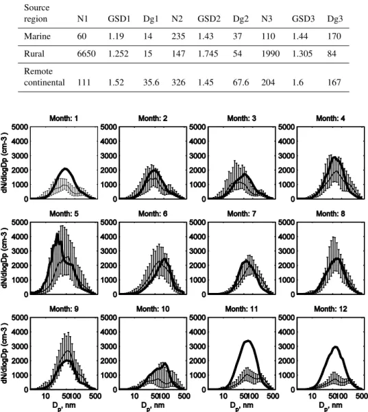
Table 2.Number of trajectories belonging to each one of the clusters
Source
region N1 GSD1 Dg1 N2 GSD2 Dg2 N3 GSD3 Dg3
Marine 60 1.19 14 235 1.43 37 110 1.44 170
Rural 6650 1.252 15 147 1.745 54 1990 1.305 84
Remote
continental 111 1.52 35.6 326 1.45 67.6 204 1.6 167
Fig. 5.Monthly median modeled size distributions (thick black line) and 25-th–75-th percentile (thin black line + errorbars) for correspiond-ing observational aerosol number size distribution data, Hyyti¨al¨a, 2000.
within the modeled 25-th–75-th percentiles of the measured results, and occasionally the modeled monthly median agrees very well with observed values (e.g. February, September, July and August). Not only the overall magnitude of the mea-sured data is captured by the model during these months but also the shape of the size distribution is properly represented, and follows the changes in observational data, i.e. towards mono- or bimodal structure. Also for year 2001 model and measurements show a good agreement, apart from January-December. This indicates that the model in general is capa-ble of reproducing the influence from relevant processes and sources. It is however obvious that the model performs worst during the winter months, especially December and January.
Table 3. Modal parameters of the input size distributions. N(1–3) corresponds to number of particles in each mode (cm−3), GSD(1– 3) correspond to the geometric standard deviation of each mode, and Dg(1–3) represents modal size in nm.
Cluster number 1 2 3 4 5 6 7 8 9 10
# trajectories 94 132 58 207 144 140 89 71 63 97
Fig. 6.Monthly median modeled size distributions (thick black line) and 25-th–75-th percentile (thin black line + errorbars) for correspiond-ing observational aerosol number size distribution data, Hyyti¨al¨a, 2001.
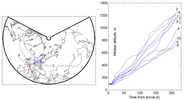
Fig. 7.The ten trajectory clusters resulting from the clustering. Cluster number is indicated at the end of each centroid (left frame). Right frame shows the median altitude along the clusters.
It may also be informative to study how the model per-forms when the air arrives from different source regions, since such an analysis could aid in finding areas where sources and/or processes are less well captured.
Fig. 8. Modelled and measured aerosol number size distribution data belonging to each on of the clusters in Fig. 7. Actual measurements at the receptor site Hyyti¨al¨a are presented as median and 25-th–75-th percentile ranges as indicated by the error bars. The thick black line corresponds to modelled median.
trajectory clustering, typical and distinct transport paths that the air follows before arriving to the receptor, maximizing the difference between the different clusters, while minimiz-ing the difference between trajectories belongminimiz-ing to a cer-tain cluster. The calculated clusters are shown in Fig. 7 as the cluster centroids (i.e. “average” trajectory of the differ-ent clusters) as well as the median height along each one of the clusters. 10 clusters have been considered in this anal-ysis. The associated number size distributions for the pe-riod February–November for both years are shown in Fig. 8. Based on the centroids, cluster 1, 2, 3, 7, and 8 are predom-inantly of marine origin and thus referred to as Marine clus-ters, clusters 5, 6, and 10 are predominantly of continental origin (Continental clusters) and clusters 9 and 4 are consid-ered to be of mixed marine-continental origin (Mixed clus-ters). The number of trajectories belonging to each cluster is shown in Table 3. All clusters show on average a descending transport pattern, but remain below 1000 m during most of the time.
During this period, the model performs well in most trans-port directions. Especially some of the marine trajectory clusters are associated with very good agreement between model and measurements (cf. Fig. 7, marine clusters 3, 7, 8, 9). The reason for just choosing February–November is that during December and January model performance is poor for most clusters, and would thus bias the otherwise satisfying
agreement between model and measurements for the rest of the year. The cause of this generally poor representation of aerosol data during winter months is not well understood, but may be linked to more complicated real world winter time meteorology which CALM is not able to capture (e.g. stabil-ity, effect of clouds etc.) or inadequate representation of the wintertime sources.
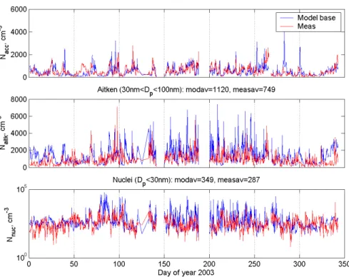
In Figs. 9 and 10 the seasonal variation of the three dom-inating size ranges (or modes) of modeled and measured data for the receptor Hyyti¨al¨a during year 2000 and 2001 is shown. This comparison considers the accumulation mode size range (Dp>100 nm, top frame), the Aitken mode size
range (30 nm<Dp<100 nm, middle frame) and the nuclei
size range (Dp<30 nm). Starting with the accumulation
Fig. 9. Modeled and observed number concentration of accumulation mode particles (Dp>100 nm, top frame), Aitken mode particles
(30< Dp<100 nm, middle frame) and nuclei mode (Dp<30 nm, bottom frame), cm−3. Blue line show modeled data and red line shows
measured concnetration. Hyyti¨al¨a, 2000.
mode provides the largest fraction of potential CCN, and thus an accurate description of this size range is of crucial im-portance for a proper determination of the important indirect aerosol effect on climate.
The seasonal variation of the Aitken mode (30<Dp <100 nm) number concentration through year
2000 is shown in the second frame of Figs. 9 and 10. As previously recognized, the model performs well especially during months 2–10, while the winter time agreement gets poorer as the model typically overestimates the Aitken mode concentration. The annual averages of modeled and measured Aitken mode concentration are 1190 cm−3 and 760 cm−3, respectively. The model result is far patchier compared to the measured data, with several high peaks throughout the year. The general trend is however satisfying. One cause that could result in the discrepancy between the model and measurements is the fact that our current single trajectory approach will be very sensitive for local point sources. As described in the method part of this study, the mass based primary aerosol emissions are transformed into a fixed size distribution (Table 1), something that also could introduce an erroneous representation of the actual size distribution emitted, resulting in disagreement between the model and measurements.
The third frame of Figs. 9 and 10 shows the modeled and measured nuclei mode (Dp<30 nm) concentration. This
figure is indicative of several interesting features related to the processes governing nucleation over Scandinavian bo-real forests. Firstly, the model overestimates the average nu-clei mode size range concentration (i.e.Dp<30nm). Annual
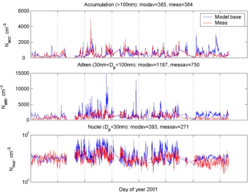
Fig. 10. Modeled and observed number concentration of accumulation mode particles (Dp>100 nm, top frame), Aitken mode particles
(30< Dp<100 nm, middle frame) and nuclei mode (Dp<30 nm, bottom frame), cm−3. Blue line show modeled data and red line shows
measured concnetration. Hyyti¨al¨a, 2001.
monoterpenes and sesquiterpenes) while nucleation is gov-erned by the concentration of H2SO4, which in turn is con-trolled by SO2emissions, condensation sink and insolation. During year 2000 also the modeled and measured trends of nuclei mode concentrations agree very well qualitatively.
It is further evident that CALM is able to reproduce the aerosol number and size with a good accuracy using only pri-mary emissions and nucleation in the lower atmosphere and neglecting the influence of free troposphere (FT) nucleation and following entrainment. This contradicts to some extent the findings from earlier global model studies which have suggested that FT can account for up to 25% of the boundary layer particle number and CCN concentration (Merikanto et al., 2009).
3.2.2 Two case studies
Two highly resolved runs were performed to investigate how the model performs in air masses arriving from the clean ma-rine sector and the polluted continental sector.
The clean period is represented by a period of 10 days in May 2000, associated with trajectories of marine origin that were advected to Hyyti¨al¨a. Nucleation is commonly ob-served over the boreal forest during spring when this type of air-mass transport dominates. As clean marine air is advected over Scandinavia, an abrupt change in sources occurs when going from the marine environment to forested areas which
to the measurements. The model predicts a distribution peak-ing around 25 nm, while in the measurements the maximum is located around 35 nm. Agreement between measured and modeled number concentrations above 100 nm is good.
The lower frame of Fig. 11 shows is the modeled time evo-lution of the aerosol size distribution at Hyyti¨al¨a during the corresponding period. As can be seen, the model is often able to capture the temporal evolution of nucleation events during most of the days. The model does however suggest nucleation taking place also 3 May (although a rather weak nucleation), which is not seen in the observational data. Es-pecially well captured are the particle formation and growth events during 1–2 May, 4–5 May and 6–7 May, although the model seems to overestimate the number of particles.
The polluted continental case was represented by 7 days in July 2001 (12–19 July), where trajectories arrived at Hyyti¨al¨a from SW in the beginning of the period, with a shift towards continental sources to the S-SE during the end of the pe-riod. The modeled and observed evolution of the size dis-tribution at Hyyti¨al¨a is shown in Fig. 13. The period is char-acterized by a persistent accumulation mode located around 100 nm, with a rather small variation in size and concentra-tion (Fig. 13, upper frame). This is a typical feature in con-tinental air as observed at Hyyti¨al¨a. Furthermore, the data show low activity of new particle formation close to the re-ceptor.
From Fig. 13, lower frame, it is seen that the model cap-tures the general properties of the variation of the size dis-tribution observed during the selected period. The modeled accumulation mode is however even more stable than obser-vations, and some peaks indicating recent new particle for-mation are present in the observational data. This feature is lacking in the modeled data. The median modeled data dur-ing this case period is shown in the right frame of Fig. 12 together with measured median and 25-th–75-th percentile range of the data.
Comparing the two case studies, it is shown that the model produces widely separate size distributions comparing the two different extremes in source areas. The marine case is associated with a high number concentration and a size distri-bution shifted towards smaller sizes, i.e. traces of recent nu-cleation. It is also clear that the model seems to overestimate the nuclei mode concentration while underestimating the growth. This could very well be a result of the way the sec-ondary organics are treated (i.e. treating first order products (15%) as very low volatile). This could result in higher con-centration of small particles due to effective growth of the freshly formed particles to more or less stable sizes. This in turn could yield a larger condensation sink, which in turn hinders consecutive growth. The continental case is associ-ated with lower number of particles, but the distribution is shifted towards the accumulation mode size range. The fact that these results agree well with observational data is en-couraging.
3.2.3 Trace gases
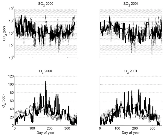
In the following we show the agreement between measured and modeled sulfur dioxide (SO2)and ozone (O3). These gases are highly important controllers of both the nucleation rate and condensation growth (via H2SO4). Ozone in turn is an important oxidant itself, and is furthermore intimately linked to the production and cycling of reactive radicals (e.g. NO3, OH, HO2). Shown in (Fig. 14) is a comparison of mea-sured and modeled [SO2] and [O3] at the SMEAR II station in Hyyti¨al¨a. In order to better see the general annual behav-ior, the data is presented as a 24 h running average to smooth out the presence of intermittent high peaks.
The annual average of measured SO2 was found to be 130 ppt for year 2000. The modeled annual average was found to be 120 ppt. During 2001 the annual average of mea-sured SO2was found to be 120 ppt, but the modeled annual average 160 ppt.
The annual average of measured O3 was found to be 28 ppb for year 2000. The modeled annual average was found to be 27 ppb. During 2001 the annual average of mea-sured O3was found to be 27 ppb, but with a modeled annual average of 26 ppb.
As can be seen in the figures both modeled and measured SO2show a pronounced seasonal variation, with maximum concentration during winter months. This is most likely the result of the combined effect of higher emissions, but also lower rate of photolytic degradation of SO2towards sulfu-ric acid. It is worth mentioning that the model appears to overestimate SO2during the winter. The seasonal variation of O3 follows an opposite pattern, with maximum concen-tration during summer months, and minimum during winter, reflecting the opposite photochemical dependence of SO2. The agreement between the model and measurement on the finer scale is not as good as for SO2, but as shown by the an-nual average the magnitude of modeled and measured ozone agrees perfectly.
The modeled concentration of monoterpenes was found to be∼80 ppt as an annual average, which is lower, but in the same range as measured literature values (e.g. (Hakola et al., 2009), which are typically below 100 ppt during winter and above 200 ppt during the middle of the summer. However, these measurements are often performed close to the canopy, whereas our modeled concentrations represent the average of the whole ML. Furthermore, we cannot exclude the possibil-ity or stronger sinks due to higher than actual abundance of OH radicals. Since the emissions are temperature dependent, the highest emissions occur during summer time. Annual av-erage for modeled isoprene was found to be 110 ppt, which is in the range, although slightly lower, compared to observed values.
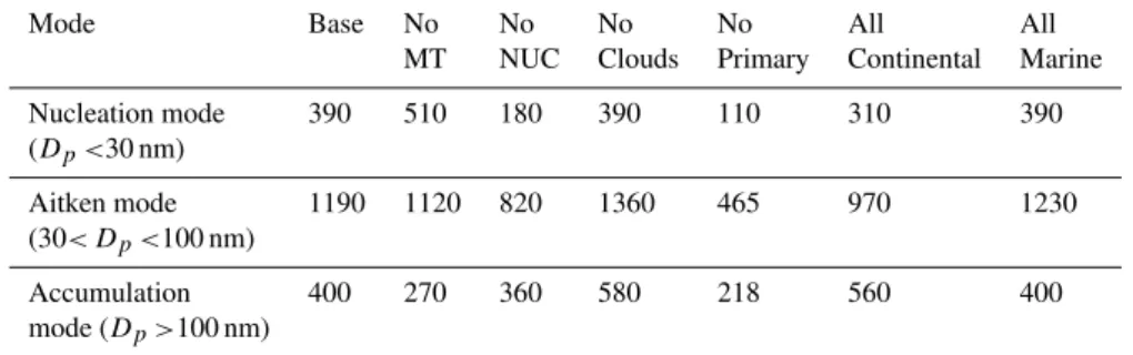
Table 4.Comparison of annual average modal concentration for different sensitivity tests and base case simulation. Shown is the median for each sensitivity test. All units in cm−3. Year 2000, Hyyti¨al¨a as receptor.
Mode Base No No No No All All
MT NUC Clouds Primary Continental Marine
Nucleation mode 390 510 180 390 110 310 390
(Dp<30 nm)
Aitken mode 1190 1120 820 1360 465 970 1230
(30< Dp<100 nm)
Accumulation 400 270 360 580 218 560 400
mode (Dp>100 nm)
noon concentrations were around 2×10⁶. This is well in the range, although slightly higher, of observations at Hyyti¨al¨a (Petaja et al., 2009, who observed 3–6×10⁵OH cm−3 dur-ing March–June).
Seasonal variation of nitrate radical is shown in the second frame of Fig. 15. The concentration is typically in the range of 107cm−3, but occasionally reaches above 108cm−3.
Sulfuric acid exhibits a typical seasonal variation, with maximum during summer months. Maximum concentrations is in the range of 1.0–1.5×107cm−3with an annual noon av-erage of 1.8×106cm−3. This agrees well with observed con-centrations at the Hyyti¨al¨a measurement station (Petaja et al., 2009).
The modeled concentration of condensable species at Hyyti¨al¨a resulting from monoterpene oxidation varies be-tween 0.2–15×107cm−3. There are no available measure-ments to confront this result, but according to e.g. (Kul-mala et al., 2001); (Spracklen et al., 2006) and references therein, investigations of new particle formation events at Hyyti¨al¨a indicate that the required concentration of condens-able species to sustain the observed growth must be around 2×10⁷–1.3×108cm−3. Thus, our results are in the lower range of these estimates.
3.3 Sensitivity tests
In this section we present the results for the sensitivity tests performed for the model. For these comparisons we have chosen year 2000. The main results are tabulated in Ta-ble 4, and will be referenced accordingly in the following text. The results of sensitivity tests with respect to nucle-ation, primary emissions, monoterpenes, clouds and precip-itation and model initialization will be shown. The results will be discussed in terms of seasons and source regions of the air parcels simulated. In order to resolve the dependence of source regions we performed a clustering of the trajecto-ries according to their typical advection paths. This will aid in the understanding of the importance of different processes at different locations/environments. The clusters for 2000 are shown in Fig. 16.
Fig. 11. Obsereved (top frame) and modeled (bottom frame) size distribution evolution. Hyyti¨al¨a, 1–10 May 2000.
3.3.1 Nucleation and primary emissions
In the model, addition of aerosols by number is controlled by either primary emitted particles (as described under Sect. 2.4.3) or nucleation and consecutive growth. The pri-mary emissions are confined to predefined size ranges, while nucleation always start with sub-nm particles formed from the gas phase. Since the number is relevant for both health and climate issues related to the atmospheric aerosol, it is of interest to investigate how the model responds to pertur-bations of these number concentration controlling processes. In this section we present results derived from three differ-ent sensitivity tests, one with nucleation completely disabled, one with an activation coefficient representing the minimum
Fig. 12. Modelled and measured number size distribution. Mea-surment data shown as median and 25-th–75-th percentile range. Model data represented by the thick solid line. Left frame, marine transport, Hyyti¨al¨a 1–10 May 2000. Right frame, continental trans-port, Hyyti¨al¨a 12–19 July 2001.
Fig. 13. Obsereved (top frame) and modeled (bottom frame) size distribution evolution. Hyyti¨al¨a, 12–19 July 2001.
By applying the range of values ofAto two different simu-lations, only very small changes in the final average size dis-tributions were noticed (not shown). This suggests that the exact value of the nucleation coefficient is insignificant for modeling on this scale. This conclusion is valid even with an order of magnitude difference inAbetween the two runs. Instead, beside the nucleation itself, the ability of the parti-cles to grow in the environment in which they are formed is of crucial importance. This ability in turn is related to the condensation sink of pre-existing particles as well as the rate of coagulation of the freshly formed particles.
Figure 17 shows the winter (October–March) and summer (April–September) average size distributions for the run with nucleation disabled and the base case distribution. Both are for year 2000. As can be clearly seen, nucleation provides the largest addition of aerosol number during the summer months, while the runs with no nucleation during the win-ter period result in virtually the same aerosol number size distribution as the base case. This is well in agreement with previous findings, showing nucleation to occur preferentially during the spring-autumn period, indicating the dependence on photochemical processes governing nucleation. As shown in Table 4, with nucleation disabled, the annual average of nuclei mode particles is decreased from 390 to 180 cm−3, the Aitken mode is reduced from 1190 to 820 cm−3and the accumulation mode is reduced from 400 to 360 cm−3. The accumulation mode typically represents the amount of avail-able CCN, and since nucleation provides∼10% of these par-ticles it is clear that nucleation provides a substantial con-tribution to potential CCN’s, also as an annual average. As shown, this contribution is most pronounced during the sum-mer period (April–September). The presence of nuclei mode particles also in the simulation where nucleation is turned off is explained by the primary emissions, contributing to sub 30 nm particles.
More interestingly, as shown in Fig. 18, the role of nu-cleation differs largely between different clusters (Fig. 16). This figure shows the summer time base case runs, together with runs with nucleation disabled. As can be seen, nucle-ation has a large impact on sub-100 nm particles in clusters 2, 4, 6, 9 and 10. Clusters 4, 6, 9 and 10 are typically as-sociated with marine air advection from north and cluster 2 centroid is directed over continental sources oriented NE of Hyyti¨al¨a. The least dependence of final size distribution on nucleation is observed in clusters 1, 5 and 8. These clusters arrive from continental sources, and both base case and the run with nucleation disabled are nearly identical. Remain-ing clusters share both continental and marine sources, and consequently there are some differences between no ation case and base case. These findings indicate that nucle-ation is an important contributor to the total aerosol number at Hyyti¨al¨a only when advection occurs from clean regions. The fact that nucleation preferentially occurs in clean, po-lar air masses has been known for several years (Boy et al., 2005; Sogacheva et al., 2008). What is interesting with these results is however, that even if nucleation is disabled over the continental region, this does not have a large impact on the resulting size distribution observed in Hyyti¨al¨a. These findings qualitatively agree with the results and discussions presented by Spracklen et al. (2006), using the global model GLOMAP. In clean regions, nucleation is a significant con-tributor to aerosol number, while in the outflow of large pol-lution sources it is not.
Fig. 14. Measured and modeled SO2concentrations in ppt (top frames) and measured and modeled O3concentration in ppb through years 2000–2001 (bottom frames), Hyyti¨al¨a, 2000–2001.
emissions affects both the summer and winter periods, al-though the difference is most pronounced for the winter pe-riod. This is opposite to the dependence on nucleation. From Fig. 20 it is also obvious that the clusters with the largest continental influence (i.e. cluster 1, 5 and 8) are most sen-sitive to the primary emissions (although insensen-sitive to nu-cleation). This means that primary emissions have a much larger impact than nucleation during these transport condi-tions. Also interesting to notice is that the clusters that were most prone to be influenced by nucleation, respond quite dif-ferently compared to their continental counterparts. This is especially evident in clusters 9 and 10, where the reduced pri-mary emissions apparently lead to an overall higher concen-tration in the nuclei mode size range (here defined as particle withDp<30 nm). This is possibly the result of lower
con-densation sink associated with the runs neglecting primary emissions, something that favors nucleation and subsequent detectable growth. During the winter period, each cluster is subject to reduction in particle number due to the absence of nucleation.
In summary this means that particle number is governed by different processes in polluted and clean environments, i.e. primary and secondary formation, respectively.
3.4 BVOC
Fig. 15.Modeled concnetrations of hydroxyl radical (OH, top left), nitrate radical (NO3, top right), sulfuric acid (H2SO4, lower left) and condensable organics (lower right). All units as cm−3, Hyyti¨al¨a 2001.
Fig. 16. Trajectory clusters centroids calculated for year 2000. Cluster number is indicated at the end of each centroid.
MT emissions. During both seasons, the number size distri-bution is shifted towards smaller sizes. This effect is most pronounced during the summer time when MT emissions are expected to be high. The shift towards smaller sizes is evi-dent in all transport directions, but most pronounced in clus-ter 9, where the sizes are not only smaller, but the number of nuclei mode particles is far higher without MT emissions as compared to the base case (not shown). MT emissions
Fig. 17.Comparison between model base case and runs with nucle-ation disabled. Two periods considered, summer (April-September, right frame) and winter (October–March, left frame), Hyyti¨al¨a, 2000.
Fig. 18.Comparison between model base case and runs with nucleation disabled per cluster. Dashed line indicate the duns with nucleation disabled, full lines represent bas case conditions, Hyyti¨al¨a, 2000.
Fig. 19. Comparison between model base case and runs with pri-mary emissions disabled. Two periods considered, summer (April– September, right frame) and winter (October–March, left frame). Hyyti¨al¨a, 2000.
3.5 Initial conditions
In order to assure that the model result isn’t biased by the initial conditions, the role of the starting size distribution and initial values of O3and NOxwas investigated in three
sepa-rate tests. Therefore, three different setups were chosen: one where all simulations are initialized with the continental type size distribution, one where all runs were initialized with the marine type size distribution and finally one test where initial O3was set to 25 ppb (i.e. 10 ppb’s less than base case condi-tions) and NOxwas set to 0.1 (i.e. 5 times less than base case conditions). The results are shown in Figs. 22–23 for con-tinental and marine starting distributions, respectively. As can be seen, if the model is initialized with only continen-tal size distributions, a shift of both wintertime and summer time average size distributions towards larger sizes is obvi-ous. However, on closer inspection with respect to the cluster orientations, it was concluded that the difference is only pro-nounced in the clean, marine clusters 4, 9, 10 (not shown). This is interpreted as the lifetime of the starting distribution in these cases being too long for the model to equilibrate to marine conditions. However, if all initial size distributions were substituted with their marine counterparts, negligible change compared to base case conditions was observed. This means that the source strength in polluted areas in principle is strong enough to allow for equilibration to continental con-ditions rather rapidly.
Fig. 20. Comparison between model base case and runs with primary emissions disabled per cluster. Dashed line indicate the duns with primary emissions disabled, full lines represent bas case conditions, Hyyti¨al¨a, 2000.
Fig. 21. Comparison between model base case and runs with monoterpene emissions disabled. Two periods considered, sum-mer (April–September, right frame) and winter (October–March, left frame), Hyyti¨al¨a, 2000.
in both ozone and OH concentration along the trajectories, and that this in turn will influence the oxidation potential and thus production of condensable species. In this test the initial concentration of O3is 10ppb less than the concentration in
Fig. 22. Comparison between model base case and runs initialized with continental distributions only. Two periods considered, sum-mer (April-September, right frame) and winter (October–March, left frame), Hyyti¨al¨a 2000.
Fig. 23. Comparison between model base case and runs initial-ized with marine distributions only. Two periods considered, sum-mer (April-September, right frame) and winter (October–March, left frame), Hyyti¨al¨a, 2000.
recovery, and it is shown in Fig. 24 that NOx for the both types of simulation gets comparable after ∼80 h, and then follow each other until arrival at the receptor. When using the lower initial values of ozone and NOxOH requires slightly more time to recover to base case values, and gets compara-ble to the base case runs (at an average of∼4×10⁻⁵cm−3) after approx. 120 h. However, the change in final size distri-bution as a result hereof is very minor and not shown. This test shows, that the initialization of the model with proper gas phase concentrations is important to get an accurate descrip-tion of the evoludescrip-tion of species such as ozone, but show at the same time that the final aerosol size distribution is largely un-affected by these moderate changes in ozone and NOx. 3.6 Clouds and precipitation
The role of clouds and precipitation was investigated by sim-ply cancelling out clouds and rain in the model scheme. The largest relative effect of this was an increase of the accu-mulation mode number concentration (Table 4) which in-creases from 400 to 580 cm−3 while the Aitken mode in-creases from 1190 to 1360 cm−3. Somehow, the nuclei mode annual average concentration remained unaffected. This probably reflects the fact that although the condensations sink increases, SO2will be more abundant due to less scav-enging by the clouds and precipitation, thus providing more nucleating material in terms of H2SO4. This indicates that clouds do play an important role in the model, and thus are necessary to achieve the observed good agreement between model and measurements during the studied period. The change is most pronounced during the summer months, al-though of similar magnitude during winter. There was no
clear (relative) dependence on source regions when perform-ing the analysis per cluster, but instead all clusters were asso-ciated with a substantial increase in the Aitken-accumulation mode size range.
3.6.1 Transport in or above mixing layer
The simplified model set-up used in this study utilize the coordinates of the trajectories to describe the movement of a quasi-1-D column consisting of a mixing layer (ML) and residual layer (RL) compartment. Thus, the model describes how the model compartments move along the latitude-longitude coordinates until the receptor station (in this case Hyyti¨al¨a) is reached. As transport path and speed may vary significantly with altitude, trajectories travelling at on average higher altitudes may not always yield a fair rep-resentation of experienced sources and transport speed of the air in the boundary layer above the receptor. On average dur-ing the simulations, the air-parcel spend 74% (or 160 h of 216 h total transport) of the time within the mixing layer. In order to test the validity of our model setup we divide the model output into two groups, one of which the air spends more than 160 h in ML and one group that spends less than 160 h in the ML. for this test we utilize only trajectories cal-culated for year 2000.
For the trajectories spending more than 160 h in the ML, the simulated average of the accumulation mode number concentrations was 480 cm−3, compared to measured aver-age of 418 cm−3. Corresponding values for the Aitken mode was found to be 1185 cm−3and 698 cm−3for modeled and measured concentration, respectively. Modelled nuclei mode concentration was found to be 314 cm−3 compared to the measured average of 245 cm−3.
In the case of less time spent in ML, the simulated av-erage of the accumulation mode number concentration was 322 cm−3, compared to measured average of 368 cm−3. Cor-responding values for the Aitken mode was found to be 1221 cm−3 and 837 cm−3 for modeled and measured con-centration, respectively. Modelled nuclei mode concentra-tion was found to be 468 cm−3 compared to the measured average of 326 cm−3.
Fig. 24. Comparisons of runs when using base case and modi-fied initial gas phase concentrations of NOxand ozone. Top frame shows the average evolution of NO + NO2along the trajectories for the low ozone (25ppb) and low NOx(0.1 ppb) (blue curve) com-pared with base case initialisation (35 ppb ozone and 0.5 ppb NOx, red curve). Bottom frame, same as above but evolution of OH is depicted.
4 Summary and conclusions
In this study we have presented a new Chemical and Aerosol Lagrangian Model (CALM) that describe the evolution of particle distribution and chemical key species along trajecto-ries and selected receptor sites. The model performs quickly enough to be run on standard PC units, and supplies users with an easy tool to investigate the relative role of aerosol dy-namic processes controlling the appearance and fate of par-ticles in the atmosphere. The model incorporates the most central aspects of the aerosol dynamics in both the dry and wet phase of the atmosphere and does as shown provide an excellent tool for determining dominating processes with a large degree of transparency and accessibility.
Considering the model performance, CALM is able to cap-ture the most prominent aspects of the observed aerosol at the Hyyti¨al¨a measurement station. This statement is valid, with the exception of the winter period, when the model per-forms poorly. The explanation for this remains open, but it may relate to a more complicated meteorology that is not captured by the trajectory model used, e.g. stratification of the lower atmosphere. It could also relate to a seasonal-ity of the sources that is not well captured by the emission module. Measured and modeled accumulation mode num-ber concentrations are similar with respect to both magni-tude and seasonal trends. This applies also to the modeled and measured nuclei mode number concentration. Investi-gation of the model results versus actual observations pro-vided a mechanistically sound explanation/description of the seasonal variation of nuclei mode particles, highlighting the
importance of balance between the generation of nucleating and condensable species and their corresponding condensa-tion sink. The model, however, seems to overestimate the Aitken mode number concentration. The poorer agreement between the measured and modeled Aitken mode particle number may be related to the way primary emissions are de-scribed. The model also performs satisfactorily in comparing either size distribution in relation to different months or dif-ferent source regions and transport routes. This indicates that the model can cope with different environments and source regions and more importantly, that the model provides a qual-itative and quantqual-itative balance between the governing pro-cesses, something that is shown by the satisfying agreement between observed and measured sulfur dioxide and the fair agreement between modeled and measured ozone, as well as reasonable representation of the concentrations of monoter-penes, isoprene, radicals and sulfuric acid.
In addition, the sensitivity of the model to different pro-cesses has been investigated in detail. The overall findings suggest that the processes are well balanced. The sensitivity tests have also provided insight into the processes governing the aerosol as observed at the Hyyti¨al¨a measurement station. These conclusions include, but are not limited to:
– Nucleation is important for the provision of particle number in clean air masses only. Under continen-tal, polluted conditions primary emissions provide most particle number.
– The model result (as represented by the receptor site Hyyti¨al¨a) proved virtually insensitive over an order of magnitude range of nucleation coefficient (4×10⁻⁷– 6×10⁻⁶s−1, activation theory, J∼[H2SO4]). This sug-gests that other processes than nucleation rate itself limit the provision of stable particles via this nucleation mechanism within this range of nucleation coefficients. This could for example be availability of condensable species and/or rate of coagulation of freshly formed par-ticles. This finding eases the selection ofAfor model-ers (The nucleation activation theory coefficientAhas been shown to vary between different environments (Ri-ipinen et al., 2007).
– Monoterpenes are an important contributor to particles above 100 nm since their oxidation products facilitates growth of particles over the entire size range. This indicates that monoterpenes may indirectly influence the radiation budget of the atmosphere. The role of monoterpenes was found to be most pronounced in the clean transport sectors of Hyyti¨al¨a.