BGD
11, 16703–16742, 2014
Oceanic N2O
emissions in the 21st century
J. Martinez-Rey et al.
Title Page
Abstract Introduction
Conclusions References
Tables Figures
◭ ◮
◭ ◮
Back Close
Full Screen / Esc
Printer-friendly Version
Interactive Discussion
Discussion
P
a
per
|
Discussion
P
a
per
|
Discussion
P
a
per
|
Discussion
P
a
per
|
Biogeosciences Discuss., 11, 16703–16742, 2014 www.biogeosciences-discuss.net/11/16703/2014/ doi:10.5194/bgd-11-16703-2014
© Author(s) 2014. CC Attribution 3.0 License.
This discussion paper is/has been under review for the journal Biogeosciences (BG). Please refer to the corresponding final paper in BG if available.
Oceanic N
2
O emissions in the 21st
century
J. Martinez-Rey1, L. Bopp1, M. Gehlen1, A. Tagliabue2, and N. Gruber3
1
Laboratoire des Sciences du Climat et de l’Environnement, IPSL, CEA/CNRS/UVSQ, Bat. 712, Orme des Merisiers, 91191 CE Saclay, Gif-sur-Yvette, France
2
School of Environmental Sciences, University of Liverpool, 4 Brownlow Street, Liverpool L69 3GP, UK
3
Environmental Physics, Institute of Biogeochemistry and Pollutant Dynamics, ETH, CHN E31.2, Universitaetstrasse 16, 8092 Zürich, Switzerland
Received: 16 September 2014 – Accepted: 15 October 2014 – Published: 4 December 2014
Correspondence to: J. Martinez-Rey ([email protected])
BGD
11, 16703–16742, 2014
Oceanic N2O
emissions in the 21st century
J. Martinez-Rey et al.
Title Page
Abstract Introduction
Conclusions References
Tables Figures
◭ ◮
◭ ◮
Back Close
Full Screen / Esc
Printer-friendly Version
Interactive Discussion
Discussion
P
a
per
|
Discussion
P
a
per
|
Discussion
P
a
per
|
Discussion
P
a
per
|
Abstract
The ocean is a substantial source of nitrous oxide (N2O) to the atmosphere, but little is
known on how this flux might change in the future. Here, we investigate the potential evolution of marine N2O emissions in the 21st century in response to anthropogenic climate change using the global ocean biogeochemical model NEMO-PISCES. We
im-5
plemented two different parameterizations of N2O production, which differ primarily at
low oxygen (O2) conditions. When forced with output from a climate model simula-tion run under the business-as-usual high CO2 concentration scenario (RCP8.5), our
simulations suggest a decrease of 4 to 12 % in N2O emissions from 2005 to 2100,
i.e., a reduction from 4.03/3.71 to 3.54/3.56 Tg N yr−1depending on the parameteriza-10
tion. The emissions decrease strongly in the western basins of the Pacific and Atlantic oceans, while they tend to increase above the Oxygen Minimum Zones (OMZs), i.e., in the Eastern Tropical Pacific and in the northern Indian Ocean. The reduction in N2O
emissions is caused on the one hand by weakened nitrification as a consequence of reduced primary and export production, and on the other hand by stronger vertical
15
stratification, which reduces the transport of N2O from the ocean interior to the ocean
surface. The higher emissions over the OMZ are linked to an expansion of these zones under global warming, which leads to increased N2O production associated
primar-ily with denitrification. From the perspective of a global climate system, the averaged feedback strength associated with the projected decrease in oceanic N2O emissions
20
amounts to around−0.009 W m−2K−1, which is comparable to the potential increase
from terrestrial N2O sources. However, the assesment for a compensation between the
BGD
11, 16703–16742, 2014
Oceanic N2O
emissions in the 21st century
J. Martinez-Rey et al.
Title Page
Abstract Introduction
Conclusions References
Tables Figures
◭ ◮
◭ ◮
Back Close
Full Screen / Esc
Printer-friendly Version
Interactive Discussion
Discussion
P
a
per
|
Discussion
P
a
per
|
Discussion
P
a
per
|
Discussion
P
a
per
|
1 Introduction
Nitrous oxide (N2O) is a gaseous compound responsible for two key feedback
mecha-nisms within the Earth’s climate. First, it acts as a long-lived and powerful greenhouse gas (Prather et al., 2012) ranking third in anthropogenic radiative forcing after car-bon dioxide (CO2) and methane (CH4) (Myrhe et al., 2013). Secondly, the ozone (O3)
5
layer depletion in the future might be driven mostly by N2O after the drastic reductions
in CFCs emissions start to show their effect on stratospheric chlorine levels
(Ravis-hankara et al., 2009). The atmospheric concentration of N2O is determined by the
nat-ural balance between sources from land and ocean and the destruction of N2O in the
atmosphere largely by reaction with OH radicals (Crutzen, 1970; Johnston, 1971). The
10
natural sources from land and ocean amount to∼6.6 and 3.8 Tg N yr−1, respectively
(Ciais et al., 2013). Anthropogenic activities currently add an additional 6.7 Tg N yr−1to
the atmosphere that caused atmospheric N2O to increase by 18 % since pre-industrial times (Ciais et al., 2013), reaching 325 ppb in the year 2012 (NOAA ESRL Global Mon-itoring Division, Boulder, Colorado, USA, http://esrl.noaa.gov/gmd/).
15
Using a compilation of 60 000 surface ocean observations of the partial pressure of N2O (pN2O), Nevison et al. (1995) computed a global ocean source of 4 Tg N yr−
1
, with a large range of uncertainty from 1.2 to 6.8 Tg N yr−1. Model derived estimates also
differ widely, i.e., between 1.7 and 8 Tg N yr−1 (Nevison et al., 2003; Suntharalingam
et al., 2000). These large uncertainties are a consequence of too few observations and
20
of poorly known N2O formation mechanisms, reflecting a general lack of understanding
of key elements of the oceanic nitrogen cycle (Gruber and Galloway, 2008; Zehr and Ward, 2002), and of N2O in particular (e.g., Zamora et al., 2012; Bange et al., 2009; Freing et al., 2012, among others). A limited number of interior ocean N2O observations
were made available only recently (Bange et al., 2009), but they contain large temporal
25
BGD
11, 16703–16742, 2014
Oceanic N2O
emissions in the 21st century
J. Martinez-Rey et al.
Title Page
Abstract Introduction
Conclusions References
Tables Figures
◭ ◮
◭ ◮
Back Close
Full Screen / Esc
Printer-friendly Version
Interactive Discussion
Discussion
P
a
per
|
Discussion
P
a
per
|
Discussion
P
a
per
|
Discussion
P
a
per
|
Basin and the Scheldt estuary, which can be used to derive and test model parameter-izations (Mantoura et al., 1993; Bange et al., 2000; Elkins et al., 1978; Yoshida et al., 1989; Punshon and Moore, 2004; De Wilde and De Bie, 2000).
N2O is formed in the ocean interior through two major pathways and consumed only in oxygen minimum zones through denitrification (Zamora et al., 2012). The first
5
production pathway is associated with nitrification (conversion of ammonia, NH+4, into nitrate, NO−
3), and occurs when dissolved O2 concentrations are above 20 µmol L− 1
. We subsequently refer to this pathway as the high-O2pathway. The second production
pathway is associated with a series of processes when O2 concentrations fall below
∼5 µmol L−1 and involve a combination of nitrification and denitrification (hereinafter 10
referred to as low-O2pathway) (Cohen and Gordon, 1978; Goreau et al., 1980; Elkins et al., 1978). As nitrification is one of the processes involved in the aerobic remineral-ization of organic matter, it occurs nearly everywhere in the global ocean with a global rate at least one order of magnitude larger than the global rate of water column denitrifi-cation (Gruber, 2008). A main reason is that denitrifidenitrifi-cation in the water column is limited
15
to the OMZs, which occupy only a few percent of the total ocean volume (Bianchi et al., 2012). This is also the only place in the water column where N2O is being consumed.
The two production pathways have very different N2O yields, i.e., fractions of
nitrogen-bearing products that are transformed to N2O. For the high-O2 pathway, the
yield is typically rather low, i.e., only about 1 in several hundred molecules of
ammo-20
nium escapes as N2O (Cohen and Gordon, 1979). In contrast, in the low-O2pathway,
and particularly during denitrification, this fraction may go up to as high as 1 : 1, i.e., that all nitrate is turned into N2O (Tiedje, 1988). The relative contribution of the two path-ways to global N2O production is not well established. Sarmiento and Gruber (2006)
suggested that the two may be of equal importance, but more recent estimates suggest
25
that the high-O2production pathway dominates global oceanic N2O production (Freing et al., 2012).
Two strategies have been pursued in the development of parameterizations for N2O
impor-BGD
11, 16703–16742, 2014
Oceanic N2O
emissions in the 21st century
J. Martinez-Rey et al.
Title Page
Abstract Introduction
Conclusions References
Tables Figures
◭ ◮
◭ ◮
Back Close
Full Screen / Esc
Printer-friendly Version
Interactive Discussion
Discussion
P
a
per
|
Discussion
P
a
per
|
Discussion
P
a
per
|
Discussion
P
a
per
|
tance of the nitrification pathway and its close association with the aerobic remineral-ization of organic matter. As a result the production of N2O and the consumption of O2
are closely tied to each other, leading to a strong correlation between the concentration of N2O and the apparent oxygen utilization (AOU). This has led to the development of two sets of parameterizations, one based on concentrations, i.e., directly as a function
5
of AOU (Butler et al., 1989) and the other based on the rate of oxygen utilization, i.e. OUR (Freing et al., 2009). Additional variables have been introduced to allow for dif-ferences in the yield, i.e., the ratio of N2O produced over oxygen consumed, such as
temperature (Butler et al., 1989) or depth (Freing et al., 2009). In the second approach, the formation of N2O is modeled more mechanistically, and tied to both nitrification
10
and denitrification by an O2 dependent yield (Suntharalingam and Sarmiento, 2000; Nevison et al., 2003; Jin and Gruber, 2003). Since most models do not include nitri-fication explicitly, the formation rate is actually coupled directly to the remineralization of organic matter. Regardless of the employed strategy, all parameterizations depend to first order on the amount of organic matter that is being remineralized in the ocean
15
interior, which is governed by the export of organic carbon to depth. The dependence of N2O production on oxygen levels and on other parameters such as temperature only acts at second order. This has important implications not only for the modeling of the present-day distribution of N2O in the ocean, but also for the sensitivity of marine N2O
to future climate change.
20
Over this century, climate change will perturb marine N2O formation in multiple ways.
Changes in productivity will drive changes in the export of organic matter to the ocean interior (Steinacher et al., 2010; Bopp et al., 2013) and hence affect the level of marine
nitrification. Ocean warming might increase the rate of N2O production during
nitrifi-cation. Changes in carbonate chemistry (Bindoffet al., 2007) might cause changes in
25
BGD
11, 16703–16742, 2014
Oceanic N2O
emissions in the 21st century
J. Martinez-Rey et al.
Title Page
Abstract Introduction
Conclusions References
Tables Figures
◭ ◮
◭ ◮
Back Close
Full Screen / Esc
Printer-friendly Version
Interactive Discussion
Discussion
P
a
per
|
Discussion
P
a
per
|
Discussion
P
a
per
|
Discussion
P
a
per
|
Models used for IPCC’s 4th assessment report estimated a decrease between 2 and 13 % in primary production (PP) under the business-as-usual high CO2concentration
scenario A2 (Steinacher et al., 2010). A more recent multi-model analysis based on the models used in IPCC’s 5th assessment report also suggest a large reduction of PP down to 18 % by 2100 for the RCP8.5 scenario (Bopp et al., 2013). In these
sim-5
ulations, the export of organic matter is projected to decrease between 6 and 18 % in 2100 (Bopp et al., 2013), with a spatially distinct pattern: in general, productivity and export are projected to decrease at mid- to low-latitudes in all basins, while productiv-ity and export are projected to increase in the high-latitudes and in the South Pacific subtropical gyre (Bopp et al., 2013). A wider spectrum of responses was reported
10
regarding changes in the ocean oxygen content. While all models simulate decreased oxygen concentrations in response to anthropogenic climate change (by about 2 to 4 % in 2100), and particularly in the mid-latitude thermocline regions, no agreement exists with regard to the hypoxic regions, i.e., those having oxygen levels below 60 µmol L−1
(Cocco et al., 2012; Bopp et al., 2013). Some models project these regions to expand,
15
while others project a contraction. Even more divergence in the results exists for the suboxic regions, i.e., those having O2concentrations below 5 µmol L−1(Keeling et al.,
2010; Deutsch et al., 2011; Cocco et al., 2012; Bopp et al., 2013), although the trend for most models is pointing towards an expansion. At the same time, practically none of the models is able to correctly simulate the current distribution of oxygen in the
20
OMZ (Bopp et al., 2013). In summary, while it is clear that major changes in ocean biogeochemistry are looming ahead (Gruber, 2011), with substantial impacts on the production and emission of N2O, our ability to project these changes with confidence is limited.
In this study, we explore the implications of these future changes in ocean physics
25
and biogeochemistry on the marine N2O cycle, and make projections of the oceanic N2O emissions from year 2005 to 2100 under the high CO2 concentration scenario
cen-BGD
11, 16703–16742, 2014
Oceanic N2O
emissions in the 21st century
J. Martinez-Rey et al.
Title Page
Abstract Introduction
Conclusions References
Tables Figures
◭ ◮
◭ ◮
Back Close
Full Screen / Esc
Printer-friendly Version
Interactive Discussion
Discussion
P
a
per
|
Discussion
P
a
per
|
Discussion
P
a
per
|
Discussion
P
a
per
|
tury translate into changes in oceanic N2O emissions to the atmosphere. To this end, we use the NEMO-PISCES ocean biogeochemical model, which we have augmented with two different N2O parameterizations, permitting us to evaluate changes in the
ma-rine N2O cycle at the process level, especially with regard to production pathways in high and low oxygen regimes. We demonstrate that while future changes in the marine
5
N2O cycle will be substantial, the net emissions of N2O appear to change relatively
little, i.e., they are projected to decrease by about 10 % in 2100.
2 Methodology
2.1 NEMO-PISCES model
Future projections of the changes in the oceanic N2O cycle were performed
us-10
ing the PISCES ocean biogeochemical model (Aumont and Bopp, 2006) in offline
mode with physical forcings derived from the IPSL-CM5A-LR coupled model (Dufresne et al., 2013). The horizontal resolution of NEMO ocean general circulation model is 2◦
×2◦cos Ø (Ø being the latitude) with enhanced latitudinal resolution at the
equa-tor of 0.5◦. PISCES is a biogeochemical model with five nutrients (NO
3, NH4, PO4, Si
15
and Fe), two phytoplankton groups (diatoms and nanophytoplankton), two zooplankton groups (micro and mesozooplankton), and two non-living compartments (particulate and dissolved organic matter). Phytoplankton growth is limited by nutrient availabil-ity and light. Constant Redfield C : N : P ratios of 122 : 16 : 1 are assumed (Takahashi et al., 1985), while all other ratios, i.e., those associated with chlorophyll, iron, and
20
silicon (Chl : C, Fe : C and Si : C) vary dynamically.
2.2 N2O parameterizations in PISCES
We implemented two different parameterizations of N2O production in NEMO-PISCES.
The first one, adapted from Butler et al. (1989) follows the oxygen consumption ap-proach, with a temperature dependent modification of the N2O yield (P.TEMP). The
BGD
11, 16703–16742, 2014
Oceanic N2O
emissions in the 21st century
J. Martinez-Rey et al.
Title Page
Abstract Introduction
Conclusions References
Tables Figures
◭ ◮
◭ ◮
Back Close
Full Screen / Esc
Printer-friendly Version
Interactive Discussion
Discussion
P
a
per
|
Discussion
P
a
per
|
Discussion
P
a
per
|
Discussion
P
a
per
|
second one is based on Jin and Gruber (2003) (P.OMZ), following the more mecha-nistic approach, i.e., it considers the different processes occurring at differing oxygen
concentrations in a more explicit manner.
The P.TEMP parameterization assumes that the N2O production is tied to nitrification only with a yield that is at first order constant. This is implemented in the model by
5
tying the N2O formation in a linear manner to O2 consumption. A small temperature
dependence is added to the yield to reflect the potential impact of temperature on metabolic rates. The production term of N2O, i.e.,J
P.TEMP
(N2O), is then mathematically
formulated as:
JP.TEMP(N2O)=(γ+θT)J(O2)consumption (1)
10
where γ is a background yield (0.53×10⁻⁴mol N2O (mol O2consumed)− 1
), θ is the temperature dependency ofγ(4.6×10⁻⁶mol N2O (mol O2)−
1
K−1),T is temperature (K),
andJ(O2)consumptionis the sum of all biological O2consumption terms within the model.
Although this parameterization is very simple, a recent analysis of N2O observations
supports such an essentially constant yield, even in the OMZ of the Eastern Tropical
15
Pacific (Zamora et al., 2012).
The P.OMZ parameterization, formulated after Jin and Gruber (2003), assumes that the overall yield consists of a constant background yield and an oxygen dependent yield. The former is presumed to represent the N2O production by nitrification, while
the latter is presumed to reflect the enhanced production of N2O at low oxygen
con-20
centrations, in part driven by denitrification, but possibly including nitrification as well. This parameterization includes the consumption of N2O in suboxic conditions. This
gives:
JP.OMZ(N2O)=(α+βf(O2))J(O2)consumption−kN2O (2)
whereαis, as in Eq. (1), a background yield (0.9×10⁻⁴mol N2O (mol O2consumed)− 1
),
25
BGD
11, 16703–16742, 2014
Oceanic N2O
emissions in the 21st century
J. Martinez-Rey et al.
Title Page
Abstract Introduction
Conclusions References
Tables Figures
◭ ◮
◭ ◮
Back Close
Full Screen / Esc
Printer-friendly Version
Interactive Discussion
Discussion
P
a
per
|
Discussion
P
a
per
|
Discussion
P
a
per
|
Discussion
P
a
per
|
is a unitless oxygen-dependent step-like modulating function, as suggested by labora-tory experiments (Goreau et al., 1980) (Fig. S1, Supplement), and k is the 1st order rate constant of N2O consumption close to anoxia (zero otherwise). For k, we have
adopted a value of 0.138 yr−1following Bianchi et al. (2012) while we set the
consump-tion regime for O2concentrations below 5 µmol L−1. 5
The P.OMZ parameterization permits us to separately identify the N2O
forma-tion pathways associated with nitrificaforma-tion and those associated with low-oxygen concentrations (nitrification/denitrification). Specifically, we consider the source term
αJ(O2)consumptionas that associated with the nitrification pathway, while we associated
the source termβf(O2)J(O2)consumption with the low-oxygen processes (Fig. S2,
Sup-10
plement).
We employ a standard bulk approach for simulating the loss of N2O to the
atmo-sphere via gas exchange. We use the formulation of Wanninkhof et al. (1992) for esti-mating the gas transfer velocity, adjusting the Schmidt number for N2O and using the solubility constants of N2O given by Weiss and Price (1980). We assume a constant
15
atmospheric N2O concentration of 284 ppb in all simulations.
2.3 Experimental design
NEMO-PISCES was first spun up during 3000 years using constant pre-industrial dy-namical forcings fields from IPSL-CM5A-LR (Dufresne et al., 2013) without activating the N2O parameterizations. This spin-up phase was followed by a 150 yr long
simu-20
lation, forced by the same dynamical fields now with N2O production and N2O sea-to-air flux embedded. The N2O concentration at all grid points was prescribed initially
to 20 nmol L−1, which is consistent with the MEMENTO database average value of
18 nmol L−1 below 1500 m (Bange et al., 2009). During the 150 yr spin-up, we
diag-nosed the total N2O production and N2O sea-to-air flux and adjusted theα,β,γ andθ
25
parameters in order to achieve a total N2O sea-to-air flux in the two parameterizations
con-BGD
11, 16703–16742, 2014
Oceanic N2O
emissions in the 21st century
J. Martinez-Rey et al.
Title Page
Abstract Introduction
Conclusions References
Tables Figures
◭ ◮
◭ ◮
Back Close
Full Screen / Esc
Printer-friendly Version
Interactive Discussion
Discussion
P
a
per
|
Discussion
P
a
per
|
Discussion
P
a
per
|
Discussion
P
a
per
|
tribution of the high-O2pathway in the P.OMZ parameterization was set to 75 % of the total N2O production. This assumption is based on growing evidence that nitrification
is the dominant pathway of N2O production on a global scale, based on estimations
considering N2O production along with water mass transport (Freing et al., 2012). Projections in NEMO-PISCES of historical (from 1851 to 2005) and future (from
5
2005 to 2100) simulated periods were done using dynamical forcing fields from IPSL-CM5A-LR. These dynamical forcings were applied in an offline mode, i.e. monthly
means of temperature, velocity, wind speed or radiative flux were used to force NEMO-PISCES. Future simulations used the business-as-usual high CO2concentration
sce-nario (RCP8.5) until year 2100. Century scale model drifts for all the
biogeochemi-10
cal variables presented, including N2O sea-to-air flux, production and inventory, were removed using an additional control simulation with IPSL-CM5A-LR pre-industrial dy-namical forcing fields from year 1851 to 2100. Despite the fact that primary production and the export of organic matter to depth were stable in the control simulation, the air–sea N2O emissions drifted (an increase of 5 to 12 % in 200 yr depending on the
pa-15
rameterization) due to the short spin-up phase (150 yr) and to the choice of the initial conditions for N2O concentrations.
3 Present-day oceanic N2O
3.1 Contemporary N2O fluxes
The model simulated air–sea N2O emissions show large spatial contrasts, with flux
20
densities varying by one order of magnitude, but with relatively small differences
be-tween the two parameterizations (Fig. 1a and b). This is largely caused by our assump-tion that the dominant contribuassump-tion (75 %) to the total N2O production in the P.OMZ
parameterization is the nitrification pathway, which is then not so different from the
P.TEMP parameterization, where it is 100 %. As a result, the major part of N2O is
pro-25
BGD
11, 16703–16742, 2014
Oceanic N2O
emissions in the 21st century
J. Martinez-Rey et al.
Title Page
Abstract Introduction
Conclusions References
Tables Figures
◭ ◮
◭ ◮
Back Close
Full Screen / Esc
Printer-friendly Version
Interactive Discussion
Discussion
P
a
per
|
Discussion
P
a
per
|
Discussion
P
a
per
|
Discussion
P
a
per
|
into the sea-to-air N2O flux without a significant meridional transport (Suntharalingam and Sarmiento, 2000).
Elevated N2O emission regions (>50 mg N m− 2
yr−1) are found in the Eastern
Trop-ical Pacific, in the northern Indian ocean, in the northwestern Pacific, in the North Atlantic and in the Agulhas Current. In contrast, low fluxes (<10 mg N m−2yr−1) are 5
simulated in the Atlantic and Pacific subtropical gyres and southern Indian Ocean. The regions of high N2O emissions are in both parameterizations generally consis-tent with the data product of Nevison et al. (1995) (Fig. 1c), especially in the equatorial latitudes. The largest discrepancies occur in the North Pacific and Southern Ocean. The high N2O emissions observed in the North Pacific are not well represented by our
10
model, with a significant shift towards the western part of the Pacific basin, similar to other modeling studies (e.g., Goldstein et al., 2003; Jin and Gruber, 2003). The OMZ, located at approximately 600 m deep in the North Pacific, might be underestimated in our model, which in turn might suppress one potential N2O source. Minor discrepancies between model and observations also occur in the Southern Ocean, a region whose
15
role in global N2O fluxes remains debated due to the lack of observations and the
occurrence of potential artifacts due to interpolation techniques (e.g., Suntharalingam and Sarmiento, 2000; Nevison et al., 2003). In particular, the modeled N2O flux
max-ima peak at around 40◦S, i.e., around 10◦N to that estimated by Nevison et al. (1995)
(Fig. 1d).
20
3.2 Contemporary N2O concentrations and the relationship to O2
The model results at present day were evaluated against the MEMENTO database (Bange et al., 2009), which contains about 25 000 measurements of co-located N2O
and dissolved O2 concentrations. Table 1 summarizes the SD and correlation coeffi
-cients for P.TEMP and P.OMZ compared to MEMENTO. The SD of the model output
25
is very similar to MEMENTO, i.e., around 16 nmol L−1of N
2O. However, the correlation
coefficients between the sampled data points from MEMENTO and P.TEMP/P.OMZ are
BGD
11, 16703–16742, 2014
Oceanic N2O
emissions in the 21st century
J. Martinez-Rey et al.
Title Page
Abstract Introduction
Conclusions References
Tables Figures
◭ ◮
◭ ◮
Back Close
Full Screen / Esc
Printer-friendly Version
Interactive Discussion
Discussion
P
a
per
|
Discussion
P
a
per
|
Discussion
P
a
per
|
Discussion
P
a
per
|
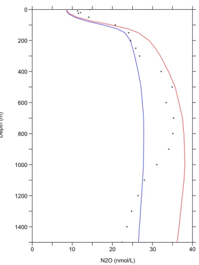
Figure 2 compares the global average vertical profile of the observed N2O against the results from the two parameterisations. The in-situ observations show three char-acteristic layers: the upper 100 m layer with low (∼10 nmol L−1) N2O concentration due
to gas exchange keeping N2O close to its saturation concentration, the mesopelagic layer, between 100 and 1500 m, where N2O is enriched via nitrification and
denitrifi-5
cation in the OMZs, and the deep ocean beyond 1500 m, with a relatively constant concentration of 18 nmol L−1 on average. Both parameterizations underestimate the
N2O concentration in the upper 100 m, where most of the N2O is potentially outgassed
to the atmosphere. In the second layer, P.OMZ shows a good correlation with the ob-servations, whereas P.TEMP is too low by∼10 nmol L−1. Below 1500 m, both parame-10
terizations simulate too high N2O compared to the observations. This may be caused by the lack or underestimation of a sink process in the deep ocean, or by the too high concentrations used to intialize the model, which persist due to the rather short spin-up time of only 150 yr.
The analysis of the model simulated N2O concentrations as a function of model
simu-15
lated O2shows the differences between the two parameterizations more clearly (Fig. 3a
and b). Such a plot allows us to assess the model performance with regard to N2O (Jin and Gruber, 2003), without being subject to the strong potential biases introduced by the model’s deficiencies in simulating the distribution of O2. This is particularly critical
in the OMZs, where all models exhibit strong biases (Cocco et al., 2012; Bopp et al.,
20
2013) (see also Fig. 3c). P.TEMP (Fig. 3a) slightly overestimates N2O for dissolved
O2 concentrations above 100 µmol L− 1
, and does not fully reproduce neither the high N2O values in the OMZs nor the N2O depletion when O2 is almost completely con-sumed. P.OMZ (Fig. 3b) overestimates the N2O concentration over the whole range
of O2, with particularly high values of N2O above 100 nmol L− 1
due to the
exponen-25
tial function used in the OMZs. There, the observations suggest concentrations below 80 nmol L−1 for the same low O
2 values, consistent with the linear trend observed for
higher O2, which seems to govern over most of the O2 spectrum, as suggested by
BGD
11, 16703–16742, 2014
Oceanic N2O
emissions in the 21st century
J. Martinez-Rey et al.
Title Page
Abstract Introduction
Conclusions References
Tables Figures
◭ ◮
◭ ◮
Back Close
Full Screen / Esc
Printer-friendly Version
Interactive Discussion
Discussion
P
a
per
|
Discussion
P
a
per
|
Discussion
P
a
per
|
Discussion
P
a
per
|
our choice of a too low N2O consumption rate under essentially anoxic conditions. The O2 distribution in the model (Fig. 3c) shows a deficient representation of the OMZs,
with higher concentrations than those from observations in the oxygen-corrected World Ocean Atlas (Bianchi et al., 2012). The rest of the O2 spectrum is well represented in our model. Finally, it should be considered that most of the MEMENTO data points are
5
from OMZs and therefore N2O measurements could be biased towards higher values
than the actual open ocean average, where our model performs better.
4 Future oceanic N2O
4.1 N2O sea-to-air flux
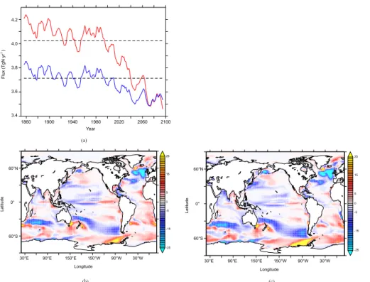
The global oceanic N2O emissions decrease relatively little over the next century
10
(Fig. 4a) between 4 and 12 %. Namely, in P.TEMP, the emissions decrease by 0.15 from 3.71 Tg N yr−1 in 1985–2005 to 3.56 Tg N yr−1 in 2080–2100 and in P.OMZ, the
decrease is slightly larger at 12 % i.e., amounting to 0.49 Tg N yr−1 from 4.03 to
3.54 Tg N yr−1. Notable is also the presence of a negative trend in N
2O emissions over
the 20th century, most pronounced in the P.OMZ parameterization. Considering the
15
change over the 20th and 21st centuries together, the decreases increase to 7 and 15 %.
These relatively small global decreases mask more substantial changes at the re-gional scale, with a mosaic of regions experiencing a substantial increase and regions experiencing a substantial decrease (Fig. 4b and c). In both parameterizations, the
20
oceanic N2O emissions decrease in the northern and south western oceanic basins (e.g., the North Atlantic and Arabian Sea), by up to 25 mg N m−2yr−1. In contrast, the
fluxes are simulated to increase in the Eastern Tropical Pacific and in the Bay of Bengal. For the Benguela Upwelling System (BUS) and the North Atlantic a bi-modal pattern emerges in 2100. As was the case for the present-day distribution of the N2O fluxes,
BGD
11, 16703–16742, 2014
Oceanic N2O
emissions in the 21st century
J. Martinez-Rey et al.
Title Page
Abstract Introduction
Conclusions References
Tables Figures
◭ ◮
◭ ◮
Back Close
Full Screen / Esc
Printer-friendly Version
Interactive Discussion
Discussion
P
a
per
|
Discussion
P
a
per
|
Discussion
P
a
per
|
Discussion
P
a
per
|
the overall similarity between the two parameterizations is a consequence of the dom-inance of the nitrification (high-O2) pathway in both parameterizations.
Nevertheless there are two regions where more substantial differences between the
two parameterizations emerge: the region overlying the oceanic OMZ at the BUS and the Southern Ocean. In particular, the P.TEMP parameterization projects a larger
en-5
hancement of the flux than P.OMZ at the BUS, whereas the emissions in the Southern Ocean are enhanced in the P.OMZ parameterization.
4.2 Drivers of changes in N2O emissions
The changes in N2O emissions may stem from a change in net N2O production,
a change in the transport of N2O from its location of production to the surface, or any
10
combination of the two, which includes also changes in N2O storage. Next we deter-mine the contribution of these mechanisms to the overall decrease in N2O emissions
that our model simulated for the 21st century.
4.2.1 Changes in N2O production
In both parameterizations, global N2O production is simulated to decrease over the
15
21st century. The total N2O production in P.OMZ decreases by 0.41 Tg N yr−1in 2080–
2100 compared to the mean value over 1985–2005 (Fig. 5a). The parameterization P.OMZ allows to isolate the contributions of high- and low-O2 and will be analysed
in greater detail in the following sections. N2O production via the high-O2 pathway in P.OMZ decreases in the same order than total production, by 0.35 Tg N yr−1 in 2080– 20
2100 compared to present. The N2O production in the low-O2regions remains almost
constant across the experiment. In P.TEMP parameterization, the reduction in N2O production is much weaker than in P.OMZ due to the effect of the increasing
tempera-ture. N2O production decreases by 0.07 Tg N yr− 1
in 2080–2100 compared to present (Fig. 5b).
BGD
11, 16703–16742, 2014
Oceanic N2O
emissions in the 21st century
J. Martinez-Rey et al.
Title Page
Abstract Introduction
Conclusions References
Tables Figures
◭ ◮
◭ ◮
Back Close
Full Screen / Esc
Printer-friendly Version
Interactive Discussion
Discussion
P
a
per
|
Discussion
P
a
per
|
Discussion
P
a
per
|
Discussion
P
a
per
|
The vast majority of the changes in the N2O production in the P.OMZ parameteri-zation is caused by the high-O2pathway with virtually no contribution from the low-O2
pathway (Fig. 5a). As the N2O production in this pathway is solely driven by changes
in the O2 consumption (Eq. 2), which in our model is directly linked to export produc-tion, the dominance of this pathway implies that primary driver for the future changes
5
in N2O production in our model is the decrease in export of organic matter (CEX). It
was simulated to decrease by 0.97 Pg C yr−1 in 2100, and the high degree of
corre-spondence in the temporal evolution of export and N2O production in Fig. 5a confirms this conclusion.
The close connection between N2O production associated with the high-O2pathway
10
and changes in export production is also seen spatially (Fig. 5c), where the spatial pat-tern of changes in export and changes in N2O production are extremely highly
corre-lated (shown by stippling). Most of the small deviations are caused by lateral advection of organic carbon, causing a spatial separation between changes in O2 consumption and changes in organic matter export.
15
As there is an almost ubiquitous decrease of export in all of the major oceanic basins except at high latitudes, N2O production decreases overall as well. Hotspots of reductions exceeding −10 mg N m−2yr−1 are found in the North Atlantic, the
west-ern Pacific and Indian basins (Fig. 5c). The fewer places where export increases, are also the locations of enhanced N2O production. For example, a moderate increase of
20
3 mg N m−2yr−1is projected in the Southern Ocean, South Atlantic and Eastern
Trop-ical Pacific. The general pattern of export changes, i.e., decreases in lower latitudes, increase in higher latitudes, is consistent generally with other model projection patterns (Bopp et al., 2013), although there exist very strong model-to-model differences at the
more regional scale.
25
Although the global contribution of the changes in the low-O2 N2O production is
small, this is the result of regionally compensating trends. In the model’s OMZs, i.e., in the Eastern Tropical Pacific and in the Bay of Bengal, a significant increase in N2O
BGD
11, 16703–16742, 2014
Oceanic N2O
emissions in the 21st century
J. Martinez-Rey et al.
Title Page
Abstract Introduction
Conclusions References
Tables Figures
◭ ◮
◭ ◮
Back Close
Full Screen / Esc
Printer-friendly Version
Interactive Discussion
Discussion
P
a
per
|
Discussion
P
a
per
|
Discussion
P
a
per
|
Discussion
P
a
per
|
15 mg N m−2yr−1. This increase is primarily driven by the expansion of the OMZs in our
model (shown by stippling), while changes in export contribute less. In effect,
NEMO-PISCES projects a 20 % increase in the hypoxic volume globally, from 10.2 to 12.3×
106km3, and an increase in the suboxic volume from 1.1 to 1.6×10⁶km3 in 2100
(Fig. 5e). Elsewhere, the changes in the N2O production through the low-O2 pathway
5
are dominated by the changes in export, thus following the pattern of the changes seen in the high-O2 pathway. Overall these changes are negative, and happen to nearly
completely compensate the increase in production in the OMZs, resulting in the near constant global N2O production by the low-O2production pathway up to year 2100.
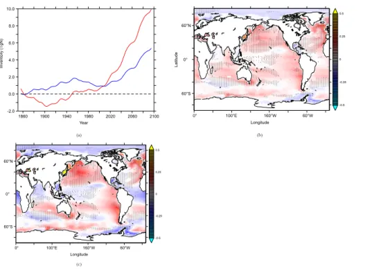
4.2.2 Changes in storage of N2O 10
A steady increase in the N2O inventory is observed from present to 2100. The pool of
oceanic N2O down to 1500 m, i.e., potentially outgassed to the atmosphere, increases
by 8.9 Tg N from 1985–2005 to year 2100 in P.OMZ, whereas P.TEMP is less sensitive to changes with an increase of 4.0 Tg N on the time period considered (Fig. 6a).
This increase in storage of N2O in the ocean interior shows an homogeneous
pat-15
tern for P.TEMP, with particular hotspots in the North Pacific, North Atlantic and the eastern boundary currents in the Pacific (Fig. 6b). The spatial variability is more pro-nounced in P.OMZ (Fig. 6c), related in part to the enhanced production associated with OMZs. Most of the projected changes in storage are associated with shoaling of the mixed layer depth (shown by stippling), suggesting that increase in N2O inventories is
20
caused by increased ocean stratification. Enhanced ocean stratification, in turn, occurs in response to increasing sea surface temperatures associated with global warming (Sarmiento et al., 2004).
4.2.3 Effects of the combined mechanisms on N2O emissions
The drivers of the future evolution of oceanic N2O emissions emerge from the
preced-25
BGD
11, 16703–16742, 2014
Oceanic N2O
emissions in the 21st century
J. Martinez-Rey et al.
Title Page
Abstract Introduction
Conclusions References
Tables Figures
◭ ◮
◭ ◮
Back Close
Full Screen / Esc
Printer-friendly Version
Interactive Discussion
Discussion
P
a
per
|
Discussion
P
a
per
|
Discussion
P
a
per
|
Discussion
P
a
per
|
organic matter remineralization reduces N2O concentrations below the euphotic zone. Secondly, the increased N2O inventory at depth is caused by increased stratification
and therefore to a less efficient transport to the sea-to-air interface, leading to a less
N2O flux.
The global changes in N2O flux, N2O production and N2O storage for P.OMZ are
5
presented in Fig. 7. Changes in N2O flux and N2O production are mostly of the same
sign in almost all of the oceanic regions in line with the assumption of nitrification being the dominant contribution to N2O production. Changes in N2O production close to the
subsurface are translated into corresponding changes in N2O flux. There is only one
oceanic region (Sub-Polar Pacific) where this correlation does not occur. N2O
inven-10
tory increases in all of the oceanic regions. The increase in inventory is particularly pronounced at low latitudes along the eastern boundary currents in the Equatorial and Tropical Pacific. Figure 7 shows how almost all the relevant changes in N2O
produc-tion and storage are related to low-latitude processes, with little or no contribuproduc-tion from changes in polar regions.
15
The synergy among the driving mechanisms can be explored with a box model pursuing two objectives. First, to reproduce future projections assuming that the only mechanisms ruling the N2O dynamics in the future were those that we have proposed
in our hypothesis, i.e., increased stratification and reduction of N2O production in
high-O2 regions. Secondly, to explore a wider range of values for both mixing (i.e., degree
20
of stratification) and efficiency of N2O production in high-O2conditions.
To this end, a box model was designed to explore the response of oceanic N2O
emissions to changes in export of organic matter (hence N2O production only in high-O2 conditions) and changes in the mixing ratio between deep (>100 m) and surface
(<100 m) layers. We divided the water column into two compartments: a surface layer
25
in the upper 100 m where 80 % of surface N2O concentration is outgassed to the atmo-sphere (Eq. 3), and a deeper layer beyond 100 m, where N2O is produced from
BGD
11, 16703–16742, 2014
Oceanic N2O
emissions in the 21st century
J. Martinez-Rey et al.
Title Page
Abstract Introduction
Conclusions References
Tables Figures
◭ ◮
◭ ◮
Back Close
Full Screen / Esc
Printer-friendly Version
Interactive Discussion
Discussion
P
a
per
|
Discussion
P
a
per
|
Discussion
P
a
per
|
Discussion
P
a
per
|
exchange is regulated by a mixing coefficientν:
surface N2O; dN2O
s
dt =−ν·
N2Os−N2Od
−κ·N2Os (3)
deep N2O;
dN2Od dt =ν·
N2Os−N2Od
+ε·ΦPOC (4)
where N2Os is N2O in the surface, N2Od is N2O in the deep reservoir, ΦPOC is the
flux of POC into the lower compartment,νis the mixing coefficient between both
com-5
partments,kis the fraction of N2O s
outgassed to the atmosphere andεthe fraction of POC leading to N2Odformation (Fig. S3 and Table S1, Supplement). Equations (3) and (4) are solved for a combination of POC fluxes and mixing coefficients, reflecting the
increasing stratification and the decrease in export production projected by year 2100 (Sarmiento et al., 2004; Bopp et al., 2013).
10
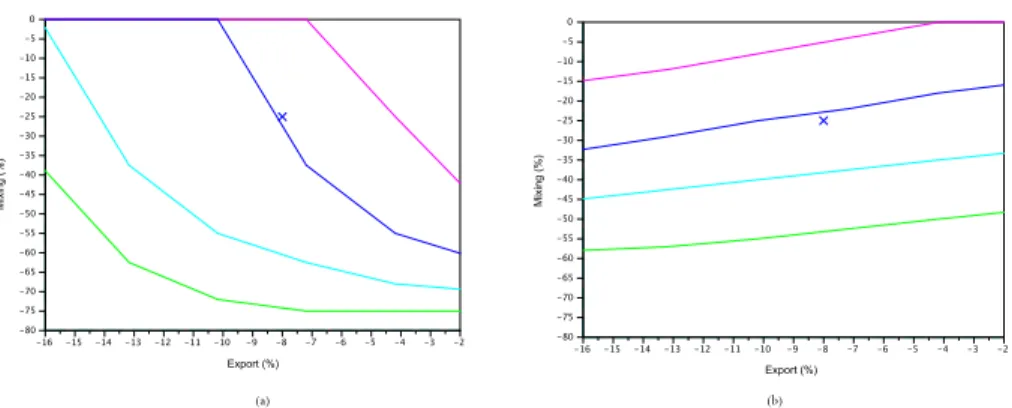
A decrease in the N2O flux is observed for a wide range of boundary conditions
simulating reduced mixing and export of POC (Fig. 8a). The equivalent of the transient NEMO-PISCES simulation, i.e., a−10 % decrease in N2O flux, is achieved for a−8 %
decrease in export in the box model. The most extreme scenario explored with the box model suggests a−20 % decrease in N2O flux, although these associated values
15
of mixing and export are clearly unrealistic, from a nearly total stagnation of ocean circulation between the deep and surface layers to an attenuation of export of−20 %
in the global ocean.
The projected increase in N2O storage in the deep reservoir is reproduced by the box model (Fig. 8b) at a wide range of changes particularly in mixing. Changes in mixing
20
dominate over changes in export as drivers of the increase in the N2O reservoir at
depth. A 25 % decrease in mixing leads to an increase in storage similar to the one projected with NEMO-PISCES (+10 %), independently of changes in export of organic
matter.
In general, the interplay between mixing and export of organic matter operates
dif-25
BGD
11, 16703–16742, 2014
Oceanic N2O
emissions in the 21st century
J. Martinez-Rey et al.
Title Page
Abstract Introduction
Conclusions References
Tables Figures
◭ ◮
◭ ◮
Back Close
Full Screen / Esc
Printer-friendly Version
Interactive Discussion
Discussion
P
a
per
|
Discussion
P
a
per
|
Discussion
P
a
per
|
Discussion
P
a
per
|
suggests that the evolution of the N2O reservoir is driven almost entirely by changes in mixing, while changes of mixing and export of organic matter have similar relevance when modulating N2O emissions.
5 Caveats in estimating N2O using ocean biogeochemical models
The use of O2consumption as a proxy for the actual N2O production expand the
un-5
certainties in N2O model estimations. Future model development should aim at the
implementation of mechanistic parameterizations of N2O production based on nitrifica-tion and denitrificanitrifica-tion rates. Further, in order to determine accurate O2boundaries for
both N2O production and N2O consumption at the core of OMZs additional
measure-ments and microbial experimeasure-ments are needed. The contribution of the high-O2pathway
10
that was considered in this model analysis might be a conservative estimate. Freing et al. (2012) suggested that the high-O2 pathway could be responsible of 93 % of the
total N2O production. Assuming that changes in the N2O flux are mostly driven by N2O production via nitrification, that would suggest a larger reduction in the marine
N2O emissions in the future. Moreover, Zamora et al. (2012) observed a higher than
15
expected N2O consumption at the core of the OMZ in the Eastern Tropical Pacific, oc-curring at an upper threshold of 10 µmol L−1. The contribution of OMZs to total N
2O
production remains an open question. N2O formation associated with OMZs might
be counterbalanced by its own local consumption, leading to the attenuation of the only increasing source of N2O attributable to the projected future expansion of OMZs
20
(Steinacher et al., 2010; Bopp et al., 2013). Finally, the accurate representation of subsurface O2concentration remains as a major challenge for ocean biogeochemical
models, as shown by Bopp et al. (2013).
The combined effect of climate change and ocean acidification has not been
an-alyzed in this study. N2O production processes might be altered by the response of
25
BGD
11, 16703–16742, 2014
Oceanic N2O
emissions in the 21st century
J. Martinez-Rey et al.
Title Page
Abstract Introduction
Conclusions References
Tables Figures
◭ ◮
◭ ◮
Back Close
Full Screen / Esc
Printer-friendly Version
Interactive Discussion
Discussion
P
a
per
|
Discussion
P
a
per
|
Discussion
P
a
per
|
Discussion
P
a
per
|
decreasing pH. This result suggests that N2O production might decrease beyond what we have estimated only due to climate change. Conversely, negative changes in the ballast effect could potentially reinforce nitrification at shallow depth in response to less
efficient POC export to depth and shallow remineralization (Gehlen et al., 2011).
Re-garding N2O formation via denitrification, changes in seawater pH as a consequence
5
of higher levels of CO2might not be substantial enough to change the N2O production
efficiency, assuming a similar response of marine denitrifiers as reported for
denitrify-ing bacteria have in terrestrial systems (Liu et al., 2010). Finally, the C : N ratio in export production (Riebesell et al., 2007) might increase in response to ocean acidification, potentially leading to a greater expansion of OMZs than simulated here (Oschlies et al.,
10
2008; Tagliabue et al., 2011), and therefore to enhanced N2O production associated with the low-O2pathway.
Changes in atmospheric nitrogen deposition have not been considered in this study. It has been suggested that due to anthropogenic activities the additional amount of reactive nitrogen in the ocean could fuel primary productivity and N2O production.
Esti-15
mates are however low, around 3–4 % of the total oceanic emissions (Suntharalingam et al., 2012).
Longer simulation periods could reveal additional effects on N2O transport beyond
changes in upwelling or meridional transport of N2O close to the subsurface
(Sunthar-alingam and Sarmiento, 2000). Eventual ventilation of the N2O reservoir at high
lati-20
tudes could shed light into the role of upwelling regions as an important source of N2O.
Additional studies using other ocean biogeochemical models might also yield alterna-tive values using the same parameterizations. N2O production is particularly sensitive to the distribution and magnitude of export of organic matter and O2 fields defined in
models.
BGD
11, 16703–16742, 2014
Oceanic N2O
emissions in the 21st century
J. Martinez-Rey et al.
Title Page
Abstract Introduction
Conclusions References
Tables Figures
◭ ◮
◭ ◮
Back Close
Full Screen / Esc
Printer-friendly Version
Interactive Discussion
Discussion
P
a
per
|
Discussion
P
a
per
|
Discussion
P
a
per
|
Discussion
P
a
per
|
6 Contribution of future N2O to climate feedbacks
Changes in the oceanic emissions of N2O to the atmosphere will have an impact on
atmospheric radiative forcing, with potential feedbacks on the climate system. Based on the estimated 4 to 12 % decrease in N2O sea-to-air flux over the 21st century
un-der RCP8.5, we estimated the feedback factor for these changes as defined by Xu-Ri
5
et al. (2012). Considering the reference value of the pre-industrial atmospheric N2O concentration of 280 ppb in equilibrium, and its associated global N2O emissions of
11.8 Tg N yr−1, we quantify the resulting changes in N
2O concentration per degree for
the two projected emissions in 2100 using P.TEMP and P.OMZ. The model projects changes in N2O emissions of−0.16 and−0.48 Tg N yr−1respectively, whereas surface 10
temperature is assumed to increase globally by 3◦C on average according to the
phys-ical forcing used in our simulations. These results yield−0.05 and−0.16 Tg N yr−1K−1,
or alternatively −1.25 and −3.8 ppb K−1 for P.TEMP and P.OMZ respectively. Using
Joos et al. (2001) we calculate the feedback factor in equilibrium for projected changes in emissions to be−0.005 and−0.014 W m−2K−1in P.TEMP and P.OMZ.
15
Stocker et al. (2013) projected changes in terrestrial N2O emissions in 2100 us-ing transient model simulations leadus-ing to feedback strengths between +0.001 and +0.015 W m−2K−1. Feedback strengths associated with the projected decrease of
oceanic N2O emissions are of the same order of magnitude as those attributable to changes in the terrestrial sources of N2O, yet opposite in sign, suggesting a
compen-20
sation of changes in radiative forcing due to future increasing terrestrial N2O emissions.
At this stage, potential compensation between land and ocean emissions is to be taken with caution, as it relies of a single model run with constant atmospheric N2O.
7 Conclusions
Our simulations suggest that anthropogenic climate change could lead to a global
de-25
de-BGD
11, 16703–16742, 2014
Oceanic N2O
emissions in the 21st century
J. Martinez-Rey et al.
Title Page
Abstract Introduction
Conclusions References
Tables Figures
◭ ◮
◭ ◮
Back Close
Full Screen / Esc
Printer-friendly Version
Interactive Discussion
Discussion
P
a
per
|
Discussion
P
a
per
|
Discussion
P
a
per
|
Discussion
P
a
per
|
crease of 12 % in marine N2O emissions for the business-as-usual high CO2emissions scenario would compensate for the estimated increase in N2O fluxes from the
terres-trial biosphere in response to anthropogenic climate change (Stocker et al., 2013), so that the climate–N2O feedback may be more or less neutral over the coming decades. The main mechanisms contributing to the reduction of marine N2O emissions are
5
a decrease in N2O production in high oxygenated waters as well as an increase in
ocean vertical stratification that acts to decrease the transport of N2O from the sub-surface to the sub-surface ocean. Despite the decrease in both N2O production and N2O
emissions, simulations suggest that the global marine N2O inventory may increase
from 2005 to 2100. This increase is explained by the reduced transport of N2O from
10
the production zones to the air–sea interface.
Differences between the two parameterizations used here are modest, and the role
of warming in P.TEMP or higher N2O yields at low-O2 concentrations in P.OMZ does
not translate into significant differences in our model projections. The dominant
high-O2N2O production pathway drives not only the general decrease in N2O emissions but
15
also the homogeneousness between the two parameterizations considered.
The N2O production pathways demand however a better understanding in order to enable an improved representation of processes in models. At a first order, the effi
-ciencies of the production processes in response to higher temperatures or increased seawaterpCO2are required. Second order effects such as changes in the O2
bound-20
aries at which nitrification and denitrification occur must be also taken into account. In the absence of process-based parameterizations, N2O production parameterizations
will still rely on export of organic carbon and oxygen levels. Both need to be improved in global biogeochemical models.
The same combination of mechanisms (i.e., change in export production and ocean
25
stratification) have been identified as drivers of changes in oceanic N2O emissions during the Younger Dryas by Goldstein et al. (2003). The N2O flux decreased, while
BGD
11, 16703–16742, 2014
Oceanic N2O
emissions in the 21st century
J. Martinez-Rey et al.
Title Page
Abstract Introduction
Conclusions References
Tables Figures
◭ ◮
◭ ◮
Back Close
Full Screen / Esc
Printer-friendly Version
Interactive Discussion
Discussion
P
a
per
|
Discussion
P
a
per
|
Discussion
P
a
per
|
Discussion
P
a
per
|
stratification. Whether these mechanisms are plausible drivers of changes beyond year 2100 remains an open question that needs to be addressed with longer simulations.
The Supplement related to this article is available online at doi:10.5194/bgd-11-16703-2014-supplement.
Acknowledgements. We thank Cynthia Nevison for providing us the N2O sea-to-air flux dataset.
5
We thank Annette Kock and Herman Bange for the availability of the MEMENTO database (https://memento.geomar.de). Comments by Parvadha Suntharalingam improved significantly this manuscript. Nicolas Gruber acknowledges the support of ETH Zürich. This work has been supported by the European Union via the Greencycles II FP7-PEOPLE-ITN-2008, number 238366. We thank Christian Ethé for help analyzing PISCES model drift.
10
References
Aumont, O. and Bopp, L.: Globalizing results from ocean in situ iron fertilization studies, Global Biogeochem. Cy., 20, GB2017, doi:10.1029/2005gb002591, 2006.
Bange, H. W., Rixen, T., Johansen, A. M., Siefert, R. L., Ramesh, R., Ittekkot, V., Hoff
-mann, M. R., and Andreae, M. O.: A revised nitrogen budget for the Arabian Sea, Global
15
Biogeochem. Cy., 14, 1283–1297, doi:10.1029/1999gb001228, 2000.
Bange, H. W., Bell, T. G., Cornejo, M., Freing, A., Uher, G., Upstill-Goddard, R. C., and Zhang, G.: MEMENTO: a proposal to develop a database of marine nitrous oxide and methane measurements, Environ. Chem., 6, 195–197, doi:10.1071/en09033, 2009.
Beman, J. M., Chow, C.-E., King, A. L., Feng, Y., Fuhrman, J. A., Andersson, A.,
20
Bates, N. R., Popp, B. N., and Hutchins, D. A.: Global declines in oceanic nitrification rates as a consequence of ocean acidification, P. Natl. Acad. Sci. USA, 108, 208–213, doi:10.1073/pnas.1011053108, 2011.
Bianchi, D., Dunne, J. P., Sarmiento, J. L., and Galbraith, E. D.: Data-based estimates of sub-oxia, denitrification, and N2O production in the ocean and their sensitivities to dissolved O2,
25
BGD
11, 16703–16742, 2014
Oceanic N2O
emissions in the 21st century
J. Martinez-Rey et al.
Title Page
Abstract Introduction
Conclusions References
Tables Figures
◭ ◮
◭ ◮
Back Close
Full Screen / Esc
Printer-friendly Version
Interactive Discussion
Discussion
P
a
per
|
Discussion
P
a
per
|
Discussion
P
a
per
|
Discussion
P
a
per
|
Bindoff, N., Willebrand, J., Artale, V., Cazenave, A., Gregory, J., Gulev, S., Hanawa, K., Le Quere, C., Levitus, S., Norjiri, Y., Shum, C., Talley, L., and Unnikrishnan, A.: Observations: oceanic climate change and sea level, in: Climate Change 2007: The Physical Science Basis. Contribution of Working Group I to the Fourth Assessment Report of the Intergovernmental Panel on Climate Change, 2007.
5
Bopp, L., Resplandy, L., Orr, J. C., Doney, S. C., Dunne, J. P., Gehlen, M., Halloran, P., Heinze, C., Ilyina, T., Séférian, R., Tjiputra, J., and Vichi, M.: Multiple stressors of ocean ecosystems in the 21st century: projections with CMIP5 models, Biogeosciences, 10, 6225– 6245, doi:10.5194/bg-10-6225-2013, 2013.
Butler, J. H., Elkins, J. W., Thompson, T. M., and Egan, K. B.: Tropospheric and dissolved N2O
10
of the west pacific and east-indian oceans during the El-Niño Southern Oscillation event of 1987, J. Geophys. Res.-Atmos., 94, 14865–14877, doi:10.1029/JD094iD12p14865, 1989. Ciais, P., Sabine, C., Bala, G., Bopp, L., Brovkin, V., Canadell, J., Chhabra, A., DeFries, R.,
Gal-loway, J., Heimann, M., Jones, C., Le Quéré, C., Myneni, R. B., Piao, S., and Thornton, P.: Carbon and other biogeochemical cycles, in: Climate Change 2013: The Physical Science
15
Basis. Contribution of Working Group I to the Fifth Assessment Report of the Intergovern-mental Panel on Climate Change, 2013.
Cocco, V., Joos, F., Steinacher, M., Frölicher, T. L., Bopp, L., Dunne, J., Gehlen, M., Heinze, C., Orr, J., Oschlies, A., Schneider, B., Segschneider, J., and Tjiputra, J.: Oxygen and indicators of stress for marine life in multi-model global warming projections, Biogeosciences, 10, 1849–
20
1868, doi:10.5194/bg-10-1849-2013, 2013.
Cohen, Y. and Gordon, L. I.: Nitrous-oxide in oxygen minimum of eastern tropical north pa-cific – evidence for its consumption during denitrification and possible mechanisms for its production, Deep-Sea Res., 25, 509–524, doi:10.1016/0146-6291(78)90640-9, 1978. Cohen, Y. and Gordon, L. I.: Nitrous-oxide production in the ocean, J. Geophys. Res.-Oceans,
25
84, 347–353, doi:10.1029/JC084iC01p00347, 1979.
Crutzen, P. J.: Influence of nitrogen oxides on atmospheric ozone content, Q. J. Roy. Meteor. Soc., 96, 320–326, doi:10.1002/qj.49709640815, 1970.
de Wilde, H. P. J. and de Bie, M. J. M.: Nitrous oxide in the Schelde estuary: production by nitrification and emission to the atmosphere, Mar. Chem., 69, 203–216,
doi:10.1016/s0304-30
4203(99)00106-1, 2000.
BGD
11, 16703–16742, 2014
Oceanic N2O
emissions in the 21st century
J. Martinez-Rey et al.
Title Page
Abstract Introduction
Conclusions References
Tables Figures
◭ ◮
◭ ◮
Back Close
Full Screen / Esc
Printer-friendly Version
Interactive Discussion
Discussion
P
a
per
|
Discussion
P
a
per
|
Discussion
P
a
per
|
Discussion
P
a
per
|
Dufresne, J. L., Foujols, M. A., Denvil, S., Caubel, A., Marti, O., Aumont, O., Balkanski, Y., Bekki, S., Bellenger, H., Benshila, R., Bony, S., Bopp, L., Braconnot, P., Brockmann, P., Cad-ule, P., Cheruy, F., Codron, F., Cozic, A., Cugnet, D., de Noblet, N., Duvel, J. P., Ethe, C., Fair-head, L., Fichefet, T., Flavoni, S., Friedlingstein, P., Grandpeix, J. Y., Guez, L., Guilyardi, E., Hauglustaine, D., Hourdin, F., Idelkadi, A., Ghattas, J., Joussaume, S., Kageyama, M.,
Krin-5
ner, G., Labetoulle, S., Lahellec, A., Lefebvre, M. P., Lefevre, F., Levy, C., Li, Z. X., Lloyd, J., Lott, F., Madec, G., Mancip, M., Marchand, M., Masson, S., Meurdesoif, Y., Mignot, J., Musat, I., Parouty, S., Polcher, J., Rio, C., Schulz, M., Swingedouw, D., Szopa, S., Ta-landier, C., Terray, P., Viovy, N., and Vuichard, N.: Climate change projections using the IPSL-CM5 Earth System Model: from CMIP3 to CMIP5, Clim. Dynam., 40, 2123–2165,
10
doi:10.1007/s00382-012-1636-1, 2013.
Elkins, J. W., Wofsy, S. C., McElroy, M. B., Kolb, C. E., and Kaplan, W. A.: Aquatic sources and sinks for nitrous-oxide, Nature, 275, 602–606, doi:10.1038/275602a0, 1978.
Freing, A., Wallace, D. W. R., Tanhua, T., Walter, S., and Bange, H. W.: North Atlantic production of nitrous oxide in the context of changing atmospheric levels, Global Biogeochem. Cy., 23,
15
GB4015, doi:10.1029/2009gb003472, 2009.
Freing, A., Wallace, D. W. R., and Bange, H. W.: Global oceanic production of nitrous oxide, Philos. T. R. Soc. B, 367, 1245–1255, doi:10.1098/rstb.2011.0360, 2012.
Gehlen, M., Gruber, N., Gangstø, R., Bopp, L., and Oschlies, A.: Biogeochemical consequences of ocean acidification and feedbacks to the earth system, in: Ocean Acidification, 230–248,
20
2011.
Goldstein, B., Joos, F., and Stocker, T. F.: A modeling study of oceanic nitrous oxide during the Younger Dryas cold period, Geophys. Res. Lett., 30, 1092, doi:10.1029/2002gl016418, 2003.
Goreau, T. J., Kaplan, W. A., Wofsy, S. C., McElroy, M. B., Valois, F. W., and Watson, S. W.:
25
Production of NO−
2 and N2O by nitrifying bacteria at reduced concentrations of oxygen, Appl. Environ. Microb., 40, 526–532, 1980.
Gruber, N.: The marine nitrogen cycle: overview of distributions and processes, in: Nitrogen in the Marine Environment, 2nd edn., 1–50, 2008.
Gruber, N.: Warming up, turning sour, losing breath: ocean biogeochemistry under global
30
change, Philos. T. R. Soc. A, 369, 1980–1996, doi:10.1098/rsta.2011.0003, 2011.