Dangerous human-made interference with climate: a GISS modelE study

(1)

ACPD

6, 12549–12610, 2006

Dangerous human-made interference with

climate

J. Hansen et al.

Title Page

Abstract Introduction

Conclusions References

Tables Figures

◭ ◮

Back Close

Full Screen / Esc

Printer-friendly Version

Interactive Discussion

Atmos. Chem. Phys. Discuss., 6, 12549–12610, 2006 www.atmos-chem-phys-discuss.net/6/12549/2006/ © Author(s) 2006. This work is licensed

under a Creative Commons License.

Atmospheric Chemistry and Physics Discussions

Dangerous human-made interference with

climate: a GISS modelE study

J. Hansen1,2, M. Sato2, R. Ruedy3, P. Kharecha2, A. Lacis1,4, R. Miller1,5, L. Nazarenko2, K. Lo3, G. A. Schmidt1,4, G. Russell1, I. Aleinov2, S. Bauer2, E. Baum6, B. Cairns5, V. Canuto1, M. Chandler2, Y. Cheng3, A. Cohen6,

A. Del Genio1,4, G. Faluvegi2, E. Fleming7, A. Friend8, T. Hall1,5, C. Jackman7, J. Jonas2, M. Kelley8, N. Y. Kiang1, D. Koch2,9, G. Labow7, J. Lerner2,

S. Menon10, T. Novakov10, V. Oinas3, Ja. Perlwitz5, Ju. Perlwitz2, D. Rind1,4, A. Romanou1,4, R. Schmunk3, D. Shindell1,4, P. Stone11, S. Sun1,11, D. Streets12, N. Tausnev3, D. Thresher4, N. Unger2, M. Yao3, and S. Zhang2

1

NASA Goddard Institute for Space Studies, New York, New York, USA

2

Columbia University Earth Institute, New York, New York, USA

3

Sigma Space Partners LLC, New York, New York, USA

4

Department of Earth and Environmental Sciences, Columbia University, New York, New York, USA

5

Department of Applied Physics and Applied Mathematics, Columbia University, New York, New York, USA

6

Clean Air Task Force, Boston, Massachusetts, USA

7

NASA Goddard Space Flight Center, Greenbelt, Maryland, USA

8

Laboratoire des Sciences du Climat et de l’Environnement, Orme des Merisiers, Gif-sur-Yvette Cedex, France

(2)

ACPD

6, 12549–12610, 2006

climate

J. Hansen et al.

Title Page

Tables Figures

◭ ◮

Back Close

Full Screen / Esc

9

Department of Geology, Yale University, New Haven, Connecticut, USA

10

Lawrence Berkeley National Laboratory, Berkeley, California, USA

11

Massachusetts Institute of Technology, Cambridge, Massachusetts, USA

12

Argonne National Laboratory, Argonne, Illinois, USA

Received: 23 October 2006 – Accepted: 28 November 2006 – Published: 5 December 2006

Correspondence to: J. Hansen (jhansen@giss.nasa.gov)

(3)

ACPD

6, 12549–12610, 2006

climate

J. Hansen et al.

Title Page

Tables Figures

◭ ◮

Back Close

Full Screen / Esc

Interactive Discussion Abstract

We investigate the issue of “dangerous human-made interference with climate” using simulations with GISS modelE driven by measured or estimated forcings for 1880–2003 and extended to 2100 for IPCC greenhouse gas scenarios as well as the “alternative”

scenario of Hansen and Sato (2004). Identification of “dangerous” effects is partly

sub-5

jective, but we find evidence that added global warming of more than 1◦C above the

level in 2000 has effects that may be highly disruptive. The alternative scenario, with

peak added forcing∼1.5 W/m2 in 2100, keeps further global warming under 1◦C if

cli-mate sensitivity is∼3◦C or less for doubled CO2. The alternative scenario keeps mean

regional seasonal warming within 2σ (standard deviations) of 20th century variability,

10

but other scenarios yield regional changes of 5–10σ, i.e., mean conditions outside the

range of local experience. We discuss three specific sub-global topics: Arctic climate change, tropical storm intensification, and ice sheet stability. We suggest that Arctic

cli-mate change has been driven as much by pollutants (O₃, its precursor CH₄, and soot)

as by CO2, offering hope that dual efforts to reduce pollutants and slow CO2 growth

15

could minimize Arctic change. Simulated recent ocean warming in the region of At-lantic hurricane formation is comparable to observations, suggesting that greenhouse gases (GHGs) may have contributed to a trend toward greater hurricane intensities. Increasing GHGs cause significant warming in our model in submarine regions of ice shelves and shallow methane hydrates, raising concern about the potential for

accel-20

erating sea level rise and future positive feedback from methane release. Growth of

non-CO2forcings has slowed in recent years, but CO2emissions are now surging well

above the alternative scenario. Prompt actions to slow CO₂ emissions and decrease

non-CO2forcings are needed to achieve the low forcing of the alternative scenario.

(4)

ACPD

6, 12549–12610, 2006

climate

J. Hansen et al.

Title Page

Tables Figures

◭ ◮

Back Close

Full Screen / Esc

Interactive Discussion 1 Introduction

The Earth’s atmospheric composition and surface properties are being altered by hu-man activities. Some of the alterations are as large or larger than natural atmosphere and surface changes, even compared with natural changes that have occurred over hundreds of thousands of years. There is concern that these human-made alterations

5

could substantially alter the Earth’s climate, which has led to the United Nations Frame-work Convention on Climate Change (United Nations, 1992) with the agreed objective “to achieve stabilization of greenhouse gas concentrations in the atmosphere at a level that would prevent dangerous anthropogenic interference with the climate system.”

The Earth’s climate system has great thermal inertia, requiring at least several

10

decades to adjust to a change of climate forcing (Hansen et al., 1984). Anthropogenic physical infrastructure giving rise to changes of atmospheric composition, such as power plants and transportation systems, also has a time constant for change of sev-eral decades. Thus there is a need to anticipate the nature of anthropogenic climate change and define the level of change constituting dangerous interference with nature.

15

Simulations with global climate models on the century time scale provide a tool for addressing that need. Climate models used for simulations of future climate must be tested by means of simulations of past climate change.

We carry out climate simulations using GISS atmospheric modelE documented by

Schmidt et al. (2006), hereaftermodelE (2006). Specifically, we attach the model III

20

version of atmospheric modelE to the computationally efficient ocean model of Russell

et al. (1995). This coupled model and its climate sensitivity have been documented

by a large set of simulations carried out to investigate the “efficacy” of various climate

forcings (Hansen et al., 2005a), hereafterEfficacy (2005). We use the same model III

here for transient climate simulations for 1880–2100, with a few simulations extended

25

to 2300.

We made calculations for each of ten individual climate forcings for the period 1880– 2003, as well as for all forcings acting together. The simulations using all ten forcings

(5)

ACPD

6, 12549–12610, 2006

climate

J. Hansen et al.

Title Page

Tables Figures

◭ ◮

Back Close

Full Screen / Esc

were extended into the future using scenarios of atmospheric composition defined by the Intergovernmental Panel on Climate Change (IPCC, 2001) and two scenarios de-fined by Hansen and Sato (2004). The simulations for 1880–2003 with individual forc-ings are described by Hansen et al. (2006b). Extensive diagnostics and convenient

graphics for all of the runs are available athttp://data.giss.nasa.gov/modelE/transient.

5

Diagnostics for extended runs with all forcings acting at once are also available from

the official IPCC repository (http://www-pcmdi.llnl.gov/ipcc/about ipcc.php).

Section 2 defines the climate model and summarizes principal known deficiencies. Section 3 defines time-dependent climate forcings that we employ. Section 4 exam-ines simulated global temperature change and specific regional climate change issues.

10

Section 5 compares trends of actual climate forcings and those in the scenarios. Sec-tion 6 summarizes the relevance of our results to the basic quesSec-tion: is there still time to avoid dangerous human interference with climate?

2 Climate model

2.1 Atmospheric model

15

The atmospheric model employed here is the 20-layer version of GISSmodelE (2006)

with 4◦×5◦ horizontal resolution. This resolution is coarse, but use of second-order

moments for numerical differencing improves the effective resolution for the transport

of tracers. The model top is at 0.1 hPa. Minimal drag is applied in the stratosphere, as needed for numerical stability, without gravity wave modeling. Stratospheric zonal

20

winds and temperature are generally realistic (Fig. 17 inEfficacy, 2005), but the polar

lower stratosphere is as much as 5–10◦_{C too cold in the winter and the model}

pro-duces sudden stratospheric warmings at only a quarter of the observed frequency.

Model capabilities and limitations are described inEfficacy(2005) andmodelE (2006).

Deficiencies are summarized below (Sect. 2.4).

25

(6)

ACPD

6, 12549–12610, 2006

climate

J. Hansen et al.

Title Page

Tables Figures

◭ ◮

Back Close

Full Screen / Esc

2.2 Ocean representation

In this paper we use the dynamic ocean model of Russell et al. (1995). One merit of this

ocean model is its efficiency, as it adds negligible computation time to that for the

atmo-sphere when the ocean horizontal resolution is the same as that for the atmoatmo-sphere, as is the case here. There are 13 ocean layers of geometrically increasing thickness,

5

four of these in the top 100 m. The ocean model employs the KPP parameterization for vertical mixing (Large et al., 1994) and the Gent-McWilliams parameterization for

eddy-induced tracer transports (Gent et al., 1995; Griffies, 1998). The resulting Russell et

al. (1995) ocean model produces a realistic thermohaline circulation (Sun and Bleck, 2006), but yields unrealistically weak El Nino-like variability as a result of its coarse

10

resolution.

Interpretation of climate simulations and observed climate change is aided by simu-lations with the identical atmospheric model attached to alternative ocean representa-tions. We make calculations with the same time-dependent 1880–2003 climate forcings of this paper and same atmospheric model attached to: (1) ocean A, which uses

ob-15

served sea surface temperature (SST) and sea ice (SI) histories of Rayner et al. (2003); (2) ocean B, the Q-flux ocean (Hansen et al., 1984; Russell et al., 1985), with specified

horizontal ocean heat transports inferred from the ocean A control run and diffusive

uptake of heat anomalies by the deep ocean; (3) ocean C, the dynamic ocean model of Russell et al. (1995); (4) ocean D, the Bleck (2002) HYCOM ocean model. Results

20

for ocean A and B are included in Hansen et al. (2006b) and on our (GISS) web site, results for ocean C are in this paper and our web site, and results for ocean D will be presented elsewhere and on our web site.

2.3 Model sensitivity

The model has sensitivity 2.7◦C for doubled CO2 when coupled to the Q-flux ocean

25

(E_fficacy, 2005), but 2.9◦_{C when coupled to the Russell et al. (1995) dynamical ocean.}

The slightly higher sensitivity with ocean C became apparent when the model run was

(7)

ACPD

6, 12549–12610, 2006

climate

J. Hansen et al.

Title Page

Tables Figures

◭ ◮

Back Close

Full Screen / Esc

extended to 1000 years, as the sea ice contribution to climate change became more im-portant relative to other feedbacks as the high latitude ocean temperatures approached

equilibrium. The 2.9◦C sensitivity corresponds to ∼0.7◦C per W/m2. In the coupled

model with the Russell et al. (1995) ocean the response to a constant forcing is such

that 50% of the equilibrium response is achieved in∼25 years, 75% in∼150 years, and

5

the equilibrium response is approached only after several hundred years. Runs of 1000 years and longer are available on the GISS web site. The model’s climate sensitivity of

2.7–2.9◦_{C for doubled CO}

2is well within the empirical range of 3±1◦C for doubled CO2

that has been inferred from paleoclimate evidence (Hansen et al., 1984, 1993; Hoffert

and Covey, 1992).

10

2.4 Principal model deficiencies

ModelE(2006) compares the atmospheric model climatology with observations. Model

shortcomings include∼25% regional deficiency of summer stratus cloud cover offthe

west coast of the continents with resulting excessive absorption of solar radiation by as

much as 50 W/m2, deficiency in absorbed solar radiation and net radiation over other

15

tropical regions by typically 20 W/m2, sea level pressure too high by 4–8 hPa in the

winter in the Arctic and 2–4 hPa too low in all seasons in the tropics,∼20% deficiency of

rainfall over the Amazon basin,∼25% deficiency in summer cloud cover in the western

United States and central Asia with a corresponding∼5◦C excessive summer warmth

in these regions. In addition to the inaccuracies in the simulated climatology, another

20

shortcoming of the atmospheric model for climate change studies is the absence of a

gravity wave representation, as noted above, which may affect the nature of interactions

between the troposphere and stratosphere. The stratospheric variability is less than

observed, as shown by analysis of the present 20-layer 4◦×5◦ atmospheric model by

J. Perlwitz (personal communication). In a 50-year control run Perlwitz finds that the

25

interannual variability of seasonal mean temperature in the stratosphere maximizes in the region of the subpolar jet streams at realistic values, but the model produces only six sudden stratospheric warmings (SSWs) in 50 years, compared with about one

(8)

ACPD

6, 12549–12610, 2006

climate

J. Hansen et al.

Title Page

Tables Figures

◭ ◮

Back Close

Full Screen / Esc

every two years in the real world.

The coarse resolution Russell ocean model has realistic overturning rates and inter-ocean transports (Sun and Bleck, 2006), but tropical SST has less east-west contrast

than observed and the model yields only slight El Nino-like variability (Fig. 17,Efficacy,

2005). Also the Southern Ocean is too well-mixed near Antarctica (Liu et al., 2003),

5

deep water production in the North Atlantic Ocean does not go deep enough, and some deep-water formation occurs in the Sea of Okhotsk region, probably because of unrealistically small freshwater input there in the model III version of modelE. Global sea ice cover is realistic, but this is achieved with too much sea ice in the Northern Hemisphere and too little sea ice in the Southern Hemisphere, and the seasonal cycle

10

of sea ice is too damped with too much ice remaining in the Arctic summer, which may

affect the nature and distribution of sea ice climate feedbacks.

Despite these model limitations, in IPCC model inter-comparisons the model used for the simulations reported here, i.e., modelE with the Russell ocean, fares about as well as the typical global model in the verisimilitude of its climatology. Comparisons

15

so far include the ocean’s thermohaline circulation (Sun and Bleck, 2006), the ocean’s heat uptake (Forest et al., 2006), the atmosphere’s annular variability and response to forcings (Miller et al., 2006), and radiative forcing calculations (Collins et al., 2006). The ability of the GISS model to match climatology, compared with other models, varies from being better than average on some fields (radiation quantities, upper tropospheric

20

temperature) to poorer than average on others (stationary wave activity, sea level pres-sure).

3 Climate forcings

Climate forcings driving our simulated climate change during 1880–2003 arise from

changing well-mixed greenhouse gases (GHGs), ozone (O3), stratospheric H2O from

25

methane (CH₄) oxidation, tropospheric aerosols, specifically, sulfates, nitrates, black

carbon (BC) and organic carbon (OC), a parameterized indirect effect of aerosols on

(9)

ACPD

6, 12549–12610, 2006

climate

J. Hansen et al.

Title Page

Tables Figures

◭ ◮

Back Close

Full Screen / Esc

clouds, volcanic aerosols, solar irradiance, soot effect on snow and ice albedos, and

land use changes. Global maps of each of these forcings for 1880–2000 are provided

inEfficacy (2005).

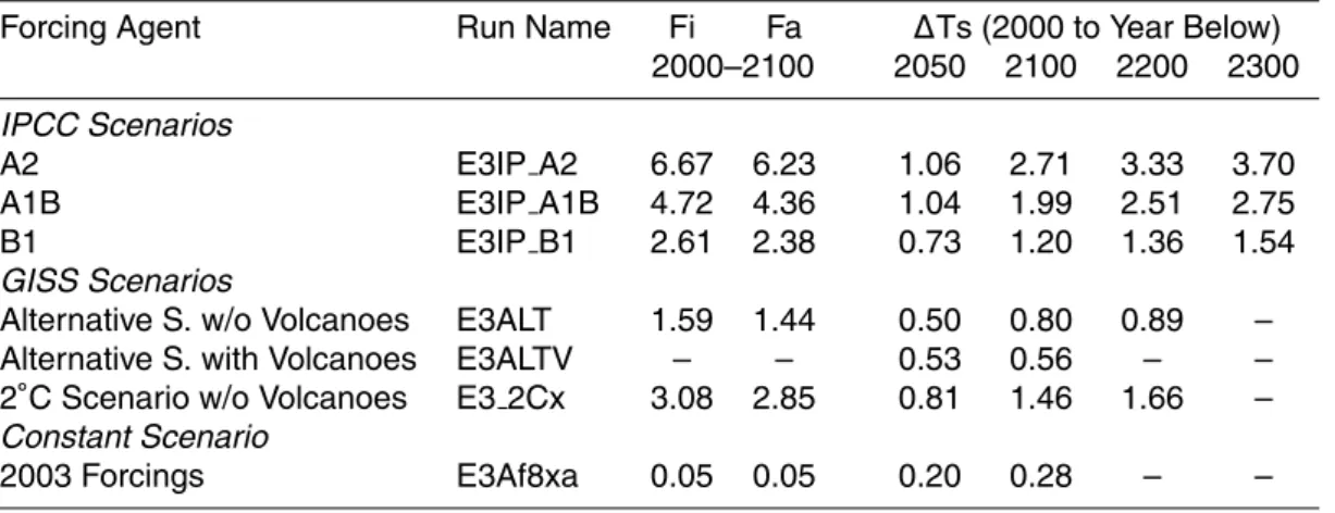
Figure 1 shows the time dependence of the global mean effective forcings. Changes

in the quantitative values of these forcings that occur with alternative forcing definitions,

5

which are small in most cases, are discussed in Efficacy (2005) and in conjunction

with the transient simulations for 1880–2003 (Hansen et al., 2006b). The predominant

forcings are due to GHGs and aerosols, including the aerosol indirect e_ffect. Ozone

forcing is significant on the century time scale, and the more uncertain solar forcing

may also be important. Volcanic effects are large on short time scales and temporal

10

clustering of volcanoes contributes to decadal variability. Soot e_ffect on snow and ice

albedos and land use change are small global forcings, but can be large on regional

scales. Efficacy (2005), this paper, and detailed simulations for 1880–2003 (Hansen

et al., 2006b) all use GHG forcings as defined in Fig. 1.

GHG climate forcing, including O3 and CH4-derived stratospheric H2O, is

15

Fe∼3 W/m2. Our partly subjective estimate of uncertainty, including imprecision in gas

amounts and radiative transfer is∼±15%, i.e.,±0.45 W/m2. Comparisons with

line-by-line radiation calculations (Collins et al., 2006) suggest that the CO2, CH4 and N2O

forcings in Model III are accurate within several percent, but the CFC forcing may be 30–40% too large. If that correction is needed, it will reduce our estimated greenhouse

20

gas forcing to Fe∼2.9 W/m2.

Stratospheric aerosol forcing following the 1991 Mount Pinatubo volcanic eruption is probably accurate within 20%, based on a strong constraint provided by satellite mea-surements of planetary radiation budget (Wong et al., 2004), as illustrated in Fig. 11 of

Efficacy (2005). The uncertainty increases for earlier eruptions, reaching about±50%

25

for Krakatau in 1883. Between large eruptions prior to the satellite era, when small eruptions might escape detection, minimum stratospheric aerosol forcing uncertainty

was∼0.5 W/m2.

Tropospheric aerosols are based on emissions estimates and aerosol transport

(10)

ACPD

6, 12549–12610, 2006

climate

J. Hansen et al.

Title Page

Tables Figures

◭ ◮

Back Close

Full Screen / Esc

eling, as described by Koch (2001). Their indirect effect is a parameterization based on

empirical e_ffects of aerosols on cloud droplet number concentration (Menon and Del

Genio, 2006) as described inEfficacy(2005). Aerosol forcings are defined in detail by

Hansen et al. (2006b). The net direct aerosol forcing is Fe=−0.60 W/m2 and the total

aerosol forcing is Fe₌₋1.37 W/m2 for 1880-2003. Our largely subjective estimate of

5

the uncertainty in the net aerosol forcing is at least 50%.

The sum of all forcings is Fe∼1.90 W/m2for 1880–2003. However, the net forcing is

evaluated more accurately from an ensemble of simulations carried out with all forcings

present at the same time (Efficacy, 2005), thus accounting for any non-linearity in the

combination of forcings and minimizing the effect of noise (unforced variability) in the

10

climate model runs. All forcings acting together yield Fe∼1.75 W/m2.

Uncertainty in the net forcing for 1880–2003 is dominated by the aerosol forcing uncertainty, which is at least 50%. Given our estimates, we must conclude that the

net forcing is uncertain by∼1 W/m2. Therefore the smallest and largest forcings within

the range of uncertainty differ by more than a factor of three, primarily because of the

15

absence of accurate measurements of aerosol direct and indirect forcings.

One implication of the uncertainty in the net 1880–2003 climate forcing is that it is fruitless to try to obtain an accurate empirical climate sensitivity from observed global temperature change of the past century. However, paleoclimate evidence of climate change between periods with well-known boundary conditions (forcings) provides a

20

reasonably precise measure of climate sensitivity: 3±16◦C for doubled CO2(Hansen et

al., 1984, 1993; Hoffert and Covey, 1992). Thus we conclude that our model sensitivity

of 2.9◦_{C for doubled CO}

2is reasonable.

Figure 1b indicates that, except for occasional large volcanic eruptions, the GHG climate forcing has become the dominant global climate forcing during the past few

25

decades. GHG dominance is a result of the slowing growth of anthropogenic aerosols, as increased aerosol amounts in developing countries have been at least partially bal-anced by decreases in developed countries. This dominance of GHG forcing, with a net forcing that may be approaching the equivalence of a 1% increase in solar

(11)

ACPD

6, 12549–12610, 2006

climate

J. Hansen et al.

Title Page

Tables Figures

◭ ◮

Back Close

Full Screen / Esc

ance, implies that global temperature change should now be rising above the level of natural climate variability.

Furthermore, we can anticipate that the dominance of GHG forcing over aerosol and other forcings will be all the more true in the future (Andreae et al., 2005). There is little expectation that developing countries will allow aerosol amounts to continue

5

to grow rapidly, as their aerosol pollution is already hazardous to human health and technologies to reduce emissions are available. If future GHG amounts are anywhere near the projections in typical IPCC scenarios, GHG climate forcings will be dominant in the future. Thus, we suggest, it is possible to make meaningful projections of future climate change despite uncertainties in past aerosol forcings.

10

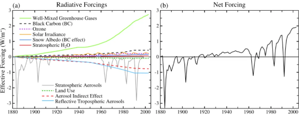
IPCC (2001) defines a broad range of scenarios for future greenhouse gas amounts. This range is shown nominally by the colored area in Fig. 2, which is bordered by the two IPCC scenarios that give the largest and smallest greenhouse gas amounts in 2100. We carry out climate simulations for three IPCC scenarios: A2, A1B and B1. A2 and B1 are, respectively, near the maximum and minimum of the range of IPCC (2001)

15

scenarios, and A1B is known as the IPCC midrange baseline scenario.

We also carry out simulations for the “alternative” and “2◦_{C” scenarios (Fig. 2) defined}

in Table 2 of Hansen and Sato (2004). CO2increases 75 ppm during 2000–2050 in the

alternative scenario; CH4decreases moderately, enough to balance a steady increase

of N₂O; chlorofluorocarbons 11 and 12 decrease enough to balance the increase of

20

all other trace gases, an assumption that is handled by having all these gases remain

constant after 2000. CO2peaks at 475 ppm in 2100 in the alternative scenario, while

CH₄ decreases to 1300 ppb. The alternative scenario is designed to keep the added

forcing at about 1 W/m2 in 2000–2050 and another 0.5 W/m2 in 2050–2100. With a

nominal climate sensitivity of 3/4◦C per W/m2 and slowly declining greenhouse gas

25

amounts after 2100, this scenario prevents global warming from exceeding 1◦C above

the global temperature in 2000, a level that Hansen (2004, 2005a,b) has argued would constitute “dangerous anthropogenic interference” with global climate.

O’Niell and Oppenheimer (2002) suggest 2◦C added global warming as a limit

(12)

ACPD

6, 12549–12610, 2006

climate

J. Hansen et al.

Title Page

Tables Figures

◭ ◮

Back Close

Full Screen / Esc

ing “dangerous anthropogenic interference”. Thus we also made climate simulations

for a scenario expected to approach but not exceed that limit. The “2◦_{C” scenario has}

CO2peak at 560 ppm in 2100 and other greenhouse gases follow the IPCC midrange

scenario A1B (seehttp://data.giss.nasa.gov/modelforce/ghgases/).

4 Climate simulations 5

Simulations for the historical period, 1880–2003, warrant careful comparison with

observations and analysis of effects of individual forcings. Results are

de-scribed in detail by Hansen et al. (2006b) and model diagnostics are available at

http://data.giss.nasa.gov/modelE/transient. We briefly summarize results relevant to

analysis of the level of future global warming that might constitute dangerous climate

10

interference.

The model driven by the forcings of Fig. 1 simulates observed 1880–2003 global temperature change reasonably well, as crudely apparent in Fig. 3a. An equally good fit to observations probably could be obtained from a model with larger sensitivity (than

2.9◦C for doubled CO2) and smaller net forcing, or a model with smaller sensitivity

15

and larger forcing, but paleoclimate evidence constrains climate sensitivity, as men-tioned above. Also our model responds realistically to the known short-term forcing by Pinatubo volcanic aerosols (Hansen et al., 2006b), and simulated global warming for the past few decades, when increasing greenhouse gases were the dominant forcing (Fig. 1), is realistic (Hansen et al., 2005b, 2006b).

20

The largest discrepancies in simulated 1880–2003 surface temperature change are deficient warming in Eurasia and excessive warming of the tropical Pacific Ocean. Hansen et al. (2006b) present evidence that the deficient Eurasian warming may be due to an excessive anthropogenic aerosol optical depth in that region. The lack of notable observed warming in the tropical Pacific could be due to increased frequency

25

or intensity of La Ninas (Cane et al., 1997), a characteristic that our present model would not be able to capture regardless of whether it was a forced or unforced change.

(13)

ACPD

6, 12549–12610, 2006

climate

J. Hansen et al.

Title Page

Tables Figures

◭ ◮

Back Close

Full Screen / Esc

Overall, simulated climate change does not agree in all details with observations, but such agreement is not expected given unforced climate variability, uncertainty in cli-mate forcings, and current model limitations. However, the clicli-mate model does a good job of simulating global temperature change from short time-scale (volcanic aerosol) to century time-scale forcings. This provides incentive to examine model results for

evi-5

dence of dangerous human-made climate effects and to investigate how these effects

depend upon alternative climate forcing scenarios.

4.1 Global temperature change

We carry out climate simulations for the 21st century and beyond for IPCC (2001)

scenarios A2, A1B, and B1 and the “alternative” and “2◦C” scenarios of Hansen et

10

al. (2000) and Hansen and Sato (2004). Simulations are continued beyond 2100 with

forcings fixed at 2100 levels as requested by IPCC, although the alternative and 2◦C

scenarios per se have a slow decline of human-made forcings after 2100.

Figure 3a and Table 1 show the simulated global mean surface air temperature change. The A2 and B1 simulations are single runs, while A1B is a 5-member

ensem-15

ble. A 5-member ensemble of runs is carried out for the alternative scenario including future volcanoes, the 2010–2100 volcanic aerosols being identical to those of 1910– 2000 in the updated Sato et al. (1993) index. Single runs are made for the alternative

and 2◦C scenarios without future volcanoes.

Global warming is 0.80◦C between 2000 and 2100 in the alternative scenario (for the

20

25-year running mean at 2100; it is 0.66◦_{C based on linear fit) and 0.89}◦_{C between}

2000 and 2200 (0.77◦C based on linear fit) with atmospheric composition fixed after

2100. The Earth is out of energy balance by∼3/4 W/m2in 2100 (∼0.4 W/m2in 2200) in

this scenario (Fig. 3b), so global warming eventually would exceed 1◦_{C if atmospheric}

composition remained fixed indefinitely. The alternative scenario of Hansen and Sato

25

(2004) has GHGs decrease slowly after 2100, thus keeping warming <1◦C. Global

warming in all other scenarios already exceeds 1◦_{C by 2100, ranging from 1.2}◦_{C in}

scenario B1 to 2.7◦C in scenario A2.

(14)

ACPD

6, 12549–12610, 2006

climate

J. Hansen et al.

Title Page

Tables Figures

◭ ◮

Back Close

Full Screen / Esc

Note the slow decline of the planetary energy imbalance after 2100 (Fig. 3b), which reflects the shape of the surface temperature response to a climate forcing. Figure 4d

inEfficacy (2005) shows that 50% of the equilibrium response is achieved within 25

years, but only 75% after 150 years, and the final 25% requires several centuries. This behavior of the coupled model occurs because the deep ocean continues to take up

5

heat for centuries. Verification of this behavior in the real world requires data on deep ocean temperature change. In the model, heat storage associated with this long tail of the response curve occurs mainly in the Southern Ocean. Measured ocean heat storage in the past decade (Willis et al., 2004; Lyman et al., 2006) presents limited evidence of this phenomenon, but the record is too short and the measurements too

10

shallow for confirmation. Ongoing simulations with modelE coupled to the current ver-sion of the Bleck (2002) ocean model do not show such deep mixing of heat anomalies, at least not so rapidly.

Figure 3c compares the global distribution of 21st century temperature change in the

five scenarios. Warming in the alternative scenario is<1◦C in most regions, reaching

15

1◦C only in the Arctic and a few continental regions. The weakest IPCC forcing, B1, has

almost twice the warming of the alternative scenario, with more than 2◦_{C in the Arctic.}

The strongest IPCC forcing, A2, yields four times the global warming of the alternative

scenario, with annual warming exceeding 4◦C on large areas of land and in the Arctic.

We compare these warmings to observed change and interannual variability in the next

20

section.

4.2 Regional climate change

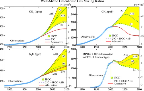
Figure 4 compares climate change simulated for the present century with climate change and climate variability that humans and the environment experienced in the past century. Figure 4a is the observed change (based on linear trend) of seasonal

25

(winter and summer) surface temperature over the past century and the local

stan-dard deviation,σ, of seasonal mean temperature about its 100-year mean. The range

(15)

ACPD

6, 12549–12610, 2006

climate

J. Hansen et al.

Title Page

Tables Figures

◭ ◮

Back Close

Full Screen / Esc

no more than twice the range shown in Fig. 4a for the past century (Mann et al., 2003). Figure 4b shows the simulated change of seasonal mean temperature this century and the ratio of this change to observed local temperature variability. Warming in the

alternative scenario is typically 2σor less, i.e., the average seasonal mean temperature

at the end of the 21st century will be at a level that is occasionally experienced in today’s

5

climate. Warming in the 2◦C and IPCC B1 scenarios is typically 4σ. Warming in the

IPCC A2 and A1B scenarios, commonly called “business-as-usual” (BAU) scenarios,

is typically 5–10σ.

Ecosystems, wildlife, and humans would be subjected in the BAU scenarios to

con-ditions far outside their local range of experience. We suggest that 5–10σ changes of

10

seasonal temperature are prima facie evidence that the BAU scenarios extend well into the range of “dangerous anthropogenic interference”.

Figure 4 provides a general perspective on the magnitude of regional climate change expected for a given climate forcing scenario. Additional perspective on the practical significance of regional climate change is obtained by considering three specific cases:

15

the Arctic, tropical storms originating in the Tropical Atlantic Ocean, and the ocean in the vicinity of ice shelves.

4.2.1 Arctic climate change

Recent warming in the Arctic is having notable effects on regional ecology, wildlife,

and indigenous peoples (ACIA, 2004). Unforced climate variability is especially large

20

in the Arctic (Fig. 4, top row), where modeled variability is similar in magnitude to observed variability (Fig. 11 in Hansen et al., 2006b). Observed variability includes

the effect of forcings, but, at least in the model, forcings are not yet large enough to

have noticeable effect on the regional standard deviation about the long-term trend.

Prior to recent warming, the largest fluctuation of Arctic temperature was the brief

25

strong Arctic warming around 1940, which Johannessen et al. (2004) and Delworth and Knutson (2000) argue was an unforced fluctuation associated with the Arctic Oscillation and a resulting positive anomaly of ocean heat inflow into that region. Forcings such

(16)

ACPD

6, 12549–12610, 2006

climate

J. Hansen et al.

Title Page

Tables Figures

◭ ◮

Back Close

Full Screen / Esc

as solar variability (Lean and Rind, 1998) or volcanoes (Overpeck et al., 1997) may contribute to Arctic variability, but we do not expect details of observed climate change in the first half of the 20th century to be matched by model simulations because of the large unforced variability. However, the magnitude of simulated Arctic warming over the entire century (illustrated by Hansen et al., 2006b) is consistent with observations.

5

Given the attribution of at least a large part of global warming to human-made forcings (IPCC, 2001), high latitude amplification of warming in climate models and paleoclimate studies, and the practical impacts of observed climate change (ACIA, 2004), Arctic climate change warrants special attention.

Early energy balance climate models revealed a “small ice cap instability” at the pole

10

(Budyko, 1969; North, 1984), which implied that, once sea ice retreated to a critical latitude, all remaining ice would be lost rapidly without additional forcing. This instability disappears in climate models with a seasonal cycle of radiation and realistic dynamical energy transports, but a vestige remains: the snow/ice albedo feedback makes sea ice cover in summer and fall sensitive to moderate increase of climate forcings. The Arctic

15

was ice-free in the warm season during the Middle Pliocene when global temperature

was only 2–3◦_{C warmer than today (Crowley, 1996; Dowsett et al., 1996).}

Satellite data indicate a rapid decline,∼9%/decade, in perennial Arctic sea ice since

1978 (Comiso, 2002), raising the question of whether the Arctic has reached a “tipping point” leading inevitably to loss of all warm season sea ice (Lindsay and Zhang, 2005).

20

Indeed, some experts suggest that “. . . there seem to be few, if any, processes or feed-backs that are capable of altering the trajectory toward this ‘super interglacial’ state” free of summer sea ice (Overpeck et al., 2005).

Could the Greenland ice sheet survive if the Arctic were ice-free in summer and fall? It has been argued that not only is ice sheet survival unlikely, but its disintegration would

25

be a wet process that can proceed rapidly (Hansen, 2004, 2005a, b). Thus an ice-free Arctic Ocean, because it may hasten melting of Greenland, may have implications for global sea level, as well as the regional environment, making Arctic climate change centrally relevant to definition of dangerous human interference.

(17)

ACPD

6, 12549–12610, 2006

climate

J. Hansen et al.

Title Page

Tables Figures

◭ ◮

Back Close

Full Screen / Esc

Are there realistic scenarios that might avoid large Arctic warming and an ice-free

Arctic Ocean? E_fficacy (2005) and Shindell et al. (2006) suggest that non-CO₂forcings

are the cause of a substantial portion of Arctic climate change, and thus reduction of these pollutants would make stabilization of Arctic climate more feasible. Investiga-tion of this topic should include simulaInvestiga-tions of future climate for plausible changes of

5

forcings that affect the Arctic. Although that is beyond the scope of our present paper,

we can make research suggestions on the basis of simulations that we have done for 1880–2003.

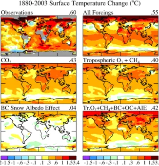
The top row of Fig. 5 shows observed 1880–2003 surface temperature change and our simulated temperature change for “all forcings”, in both cases the Arctic warming

10

being about twice the global warming. The second row shows the results of simulations

including only the CO2forcing (left) and only CH4plus tropospheric O3(right). CO2and

CH4+O3 yield comparable global and Arctic warmings. The sum of the responses to

CO₂and CH₄₊O₃exceeds either observed warming or the simulated warming for “all

forcings”, because the real world and “all forcings” include negative forcings, which are

15

due primarily to aerosols.

The lower left of Fig. 5 shows the simulated temperature change due to the effect

of black carbon on snow albedo. In this simulation, described in detail by Hansen

et al. (2006b), a moderate snow albedo forcing (∼0.05 W/m2) is assumed. The BC

producing this snow albedo effect also has direct and indirect aerosol forcings, and the

20

sources producing BC also produce OC. The lower right of Fig. 5 shows the simulated

temperature change due to the combination of CH4+O3+BC+OC, including aerosol

direct and indirect forcings and the snow albedo effect. The global warming is about the

same as that due to CH4+O3, as the warming by BC and its snow albedo effect is not

much larger than the cooling by OC and the indirect effect of BC and OC. Nevertheless,

25

simulated Arctic warming is more than 1◦_{C with all of these forcings present.}

If CO2 growth in the 21st century is kept as small as in the alternative scenario,

ad-ditional Arctic warming is only∼1◦C (Fig. 3c). Thus, in that case, reduction of some of

the pollutants considered in Fig. 5 may make it possible to keep further Arctic warming

(18)

ACPD

6, 12549–12610, 2006

climate

J. Hansen et al.

Title Page

Tables Figures

◭ ◮

Back Close

Full Screen / Esc

under 1◦_{C and thus probably avoid loss of all sea ice. On the other hand, if CO}

2growth

follows a BAU scenario, the impact of reducing the non-CO2 forcings will be small by

comparison and probably inconsequential.

We suggest that the conclusion that a “tipping point” has been passed, such that it is not possible to avoid a warm-season ice-free Arctic, with all that might entail for

5

regional climate and the Greenland ice sheet, is not warranted yet. Better information is needed on the present magnitude of all anthropogenic forcings and on the potential

for their reduction. If CO2 growth is kept close to that of the alternative scenario, and

if strong efforts are made to reduce positive non-CO2 forcings, it may be possible to

minimize further Arctic climate change.

10

4.2.2 Tropical climate change

The tropical Atlantic Ocean is the spawning grounds for tropical storms and hurricanes that strike the United States and Caribbean nations. Many local and large-scale factors

a_ffect storm activity and there are substantial correlations of storm occurrence and

severity with external conditions such as the Southern Oscillation and Quasi-Biennial

15

Oscillation (Gray, 1984; Emanuel, 1987; Henderson-Sellers et al., 1998; Goldenberg, et al., 2001; Trenberth, 2005). Two factors especially important for Atlantic hurricane

activity are SST at 10–20◦N, the main development region (MDR) for Atlantic tropical

storms (Goldenberg, et al., 2001), and the absence of strong vertical wind shear that would inhibit cyclone formation. In addition, SST and ocean temperature to a few

20

hundred meters depth along the hurricane track play a role in storm intensity, because warm waters enhance the potential for the moist convection that fuels the storm, while cooler waters at depth stirred up by the storm can dampen its intensity.

Some measures of Atlantic hurricane intensity and duration increased in recent years, raising concern that global warming may be a factor in this trend (Bell et al.,

25

2005; Webster et al., 2005, Emanuel, 2005). However, Gray (2005) and the director of the United States National Hurricane Center (Mayfield, 2005), while acknowledg-ing a connection between ocean temperature and hurricanes, reject the suggestion

(19)

ACPD

6, 12549–12610, 2006

climate

J. Hansen et al.

Title Page

Tables Figures

◭ ◮

Back Close

Full Screen / Esc

that global warming has contributed to the recent storm upsurge, citing instead natu-ral cycles of Atlantic Ocean temperature. Indeed, multi-decadal variations of Atlantic Ocean temperatures are found in instrumental data (Kushnir, 1994), in paleoclimate proxy temperatures (Mann et al., 1998), and in coupled atmosphere-ocean climate simulations without external forcing (Delworth and Mann, 2000). However, Mann and

5

Emanuel (2006) argue that SST fluctuations in the MDR associated with the Atlantic Multi-decadal Oscillation are statistical artifacts, and that practically all SST variability in the region can be attributed to competing trends in greenhouse gases and aerosols. Climate forcings also contribute to ocean temperature change, so it is of interest to compare modeled temperature change due to forcings with observed temperature

10

change in regions and season relevant to tropical storms. Bell et al. (2005) define an Accumulated Cyclone Energy (ACE) index that accounts for the combined strength and duration of tropical storms of hurricanes originating in the Atlantic Ocean. This index (Fig. 4.5 of Bell et al., 2005) was generally low during 1970–1994. For the past decade the ACE index has been a factor 2.4 higher than in 1970–1994. Perhaps not

15

coincidentally, the index had peaks near 1980 and 1990, when global temperature also

had peaks, and the index was low during the few years affected by the 1991 Pinatubo

global cooling. The past decade, when ACE is highest, is the warmest time in the past century and a period with rapid uptake of heat by the ocean (Levitus et al., 2005; Willis et al., 2004; Hansen et al., 2005b; Lyman et al., 2006).

20

Figure 6a shows SST anomalies in 1995–2005, the time of high hurricane inten-sity, relative to 1970–1994, when Atlantic Ocean and Gulf of Mexico hurricanes were

weaker. Observations have warming∼0.2◦C in the Gulf of Mexico and∼0.45◦C in the

MDR. The ensemble mean of the simulation with standard “all forcings” has

warm-ing about 0.35◦C in both regions, suggesting that much, perhaps most, of observed

25

warming in these critical regions is due to the forcings that drive the climate model. Increasing GHGs, the principal forcing driving the model toward warming (Fig. 1), are known accurately, but other forcings have large uncertainties. Thus we performed

ad-ditional simulations in which the most uncertain forcings were altered to test the effect

(20)

ACPD

6, 12549–12610, 2006

climate

J. Hansen et al.

Title Page

Tables Figures

◭ ◮

Back Close

Full Screen / Esc

of uncertainties and to provide more fodder for examining statistical significance. The lower three rows in Fig. 6a (and c) show results for three 5-member ensem-bles of model runs with altered tropospheric aerosol and solar forcings, as described in detail by Hansen et al. (2006b). In AltAer1 anthropogenic sulfate aerosols have the identical time dependence as in the standard experiment (Fig. 1) but the anthropogenic

5

increase is reduced by 50%. AltAer2 adds to AltAer1 a doubling of the temporal in-crease of biomass burning aerosols. AltSol replaces the solar irradiance history of Lean (2000), which includes both long-term and solar cycle variations, with the time series of Lean et al. (2002), which retains only the solar change due to the 11-year Schwabe cycle. These alternative forcings all yield ensemble-mean SST warmings in

10

the MDR comparable to that with standard forcings.

Figure 6b shows the 1995–2005 temperature anomalies in the five individual runs with “all forcings”, each of which yields warming in both the Gulf of Mexico and the

MDR. Figure 6c shows the standard deviationsσ* among successive 10-year periods

relative to the preceding 25 years within the available relevant period of record (1900–

15

1994). As expected, the model has too little variability at low latitudes, but it is more realistic at middle and high latitudes (the small “observed” SST variability at the highest

latitudes is an artificial result of specifying a fixed SST if any sea ice is present). σ* is

∼0.15◦C in the Gulf of Mexico in observations and model. Observedσ* is ∼0.25◦C in

the MDR, but only about half that large in the model.

20

In summary, the warming in the model in recent decades is due to the assumed forc-ings, and Hansen et al. (2006b) present evidence that the magnitude of the model’s response to forcings is realistic on time scales from that for individual volcanic erup-tions to multidecadal GHG increases. The period 1970–2005 under discussion with regard to hurricanes is the time when forcings are known most accurately, and during

25

that period anthropogenic GHGs were the dominant forcing. Although unforced fluc-tuations undoubtedly contribute to Atlantic Ocean temperature change, the expected GHG warming is comparable in magnitude to observed warming and must be at least a significant contributor to that warming.

(21)

ACPD

6, 12549–12610, 2006

climate

J. Hansen et al.

Title Page

Tables Figures

◭ ◮

Back Close

Full Screen / Esc

We conclude that the definitive assertion of Gray (2005) and Mayfield (2005), that human-made GHGs play no role in the Atlantic Ocean temperature changes that they assume to drive hurricane intensification, is untenable. Specifically, the assertions that (1) hurricane intensification of the past decade is due to changes in SST in the Atlantic Ocean, and (2) global warming cannot have had a significant role in the hurricane

5

intensification of the past decade, are mutually inconsistent. On the contrary, although natural cycles play a role in changing Atlantic SST, our model results indicate that, to the degree that hurricane intensification of the past decade is a product of increasing SST in the Atlantic Ocean and the Gulf of Mexico, human-made GHGs probably are a substantial contributor, as also concluded by Mann and Emanuel (2006). Santer et

10

al. (2006) have obtained similar conclusions by examining the results of 22 climate models.

Figure 6d shows the additional SST warming during hurricane season by

mid-century in the three IPCC, alternative, and 2◦_{C scenarios, relative to the present. SST}

is only one of the environmental factors that affect hurricanes, but there is

theoreti-15

cal (Emanuel, 1987) and empirical evidence (Emanuel, 2005; Webster et al., 2005) that higher SST contributes to increased maximum strength of tropical cyclones. The salient point that we note in Fig. 6d is that, despite the fact that warming “in the pipeline” in 2004 is the same for all scenarios, the alternative scenario already at mid-century has notably less warming than the other scenarios. This result refutes the common

20

statement that constraining climate forcings has a negligible effect on expected

warm-ing this century. Divergence of warmwarm-ing among the scenarios is even greater in later decades, as the growth of climate forcing declines rapidly in the alternative scenario.

4.2.3 Ice sheet and methane hydrate stabilities

Perhaps the greatest threat of catastrophic climate impacts for humans is the possibility

25

that warming may cause one or more of the ice sheets to become unstable, initiating a process of disintegration that is out of humanity’s control. We focus on ice sheet stability, because of the potential for sea level change this century. However, ice sheets

(22)

ACPD

6, 12549–12610, 2006

climate

J. Hansen et al.

Title Page

Tables Figures

◭ ◮

Back Close

Full Screen / Esc

are related to the stability of methane hydrates in permafrost and in marine sediments,

because ice sheet disintegration and methane release are both a_ffected by surface

warming at high latitudes and by ocean warming at the depths that affect ice shelves

and shallow methane hydrate deposits. Also, a substantial positive climate feedback

from methane release could make it di_fficult to achieve the relatively benign alternative

5

scenario, thus affecting the ice sheet stability issue as well as other climate impacts.

Most methane hydrates in marine sediments are at depths beneath the ocean floor that would require centuries for destabilization (Kvenvolden and Lorenson, 2001; Archer, 2006), but the anthropogenic thermal burst in ocean temperatures is likely to persist for centuries. Furthermore, the methane in shallow sediments, i.e., at or near the sea

10

floor, might begin to yield a positive climate feedback this century if substantial warm thermal anomalies penetrate to the ocean bottom.

The Greenland and Antarctic ice sheets contain enough water to raise sea level about 70 m, with Greenland and West Antarctica each containing about 10% of the total and East Antarctica holding the remaining 80%. IPCC (2001) central estimates for sea

15

level change in the 21st century include negligible contributions from Greenland and Antarctica, as they presume that melting of ice sheet fringes will be largely balanced by ice sheet growth in interior regions where snowfall increases.

However, Earth’s history shows that the long-term response to global warming in-cludes substantial melting of ice and sea level rise. During the penultimate interglacial

20

period, ∼130 000 years ago, when global temperature may have been as much as

∼1◦C warmer than in the present interglacial period, sea level was 4±2 m higher than

today (McCulloch and Esat, 2000; Thompson and Goldstein, 2005), demonstrating that today’s sea level is not particularly favored. However, changes of sea level and global temperature among recent interglacial periods are not large compared to the

25

uncertainties, and ice sheet stability is affected not only by global temperature but also

by the geographical and season distribution of solar irradiance, which differ from one

interglacial period to another. Therefore, it is difficult to use the last interglacial period

as a measure of the sensitivity of sea level to global temperature. The most recent

(23)

ACPD

6, 12549–12610, 2006

climate

J. Hansen et al.

Title Page

Tables Figures

◭ ◮

Back Close

Full Screen / Esc

time with global temperature∼3◦C greater than today (during the Pliocene,∼3 million

years ago) had sea level 25±10 m higher than today (Barrett et al., 1992; Dowsett et

al., 1994; Dwyer et al., 1995), suggesting that, given enough time, a BAU level of global warming could yield huge sea level change. A principal issue is thus the response time of ice sheets to global warming.

5

It is commonly assumed, perhaps because of the time scale of the ice ages, that the response time of ice sheets is millennia. Indeed, ice sheet models designed to in-terpret slow paleoclimate changes respond lethargically, i.e., on millennial time scales. However, perceived paleoclimate change may reflect more the time scale for changes of forcing, rather than an inherent ice sheet response time. Ice sheet models used for

10

paleoclimate studies generally do not incorporate all the physics that may be critical for the wet process of ice sheet disintegration, e.g., modeling of the ice streams that

chan-nel flow of continental ice to the ocean, including effects of melt percolation through

crevasses and moulins, removal of ice shelves by the warming ocean, and dynamical propagation inland of the thinning and retreat of coastal ice. Hansen (2005a, b) argues

15

that, for a forcing as large as that in BAU climate forcing scenarios, a large ice sheet response would likely occur within centuries, and ice melt this century could yield sea level rise of 1 m or more and a dynamically changing ice sheet that is out of our control. Two regional climate changes particularly relevant to ice sheet response time are: (1) surface melt on the ice sheets, and (2) melt of submarine ice shelves that buttress

20

glaciers draining the ice sheets. Zwally et al. (2002) showed that increased surface melt on Greenland penetrated ice sheet crevasses and reached the ice sheet base, where it lubricated the ice-bedrock interface and accelerated ice discharge to the ocean. Van den Broeke (2005) found that unusually large surface melt on an Antarctic ice shelf preceded and probably contributed significantly to collapse of the ice shelf. Thinning

25

and retreat of ice shelves due to warming ocean water works in concert with surface melt. Hughes (1972, 1981) and Mercer (1978) suggested that floating and grounded ice shelves extending into the ocean serve to buttress outlet glaciers, and thus a warm-ing ocean that melts ice shelves could lead to rapid ice sheet shrinkage or collapse.

(24)

ACPD

6, 12549–12610, 2006

climate

J. Hansen et al.

Title Page

Tables Figures

◭ ◮

Back Close

Full Screen / Esc

Confirmation of the effectiveness of these processes has been obtained in the past

decade from observations of increased surface melt, ice shelf thinning and retreat, and acceleration of glaciers on the Antarctic Peninsula (De Angelis and Skvarca, 2003; Rig-not et al., 2004; van den Broeke, 2005), West Antarctica (RigRig-not, 1998; Shepherd et al., 2002, 2004; Thomas et al., 2004), and Greenland (Abdalati et al., 2001; Zwally et

5

al., 2002; Thomas et al., 2003), in some cases with documented effects extending far

inland. Thus we examine here both projected surface warming on the ice sheets and warming of nearby ocean waters.

Summer surface air temperature change on Greenland in the 21st century is only

0.5–1◦C with alternative scenario climate forcings (Fig. 4), but it is 2–4◦C for the IPCC

10

BAU scenarios (A2 and A1B). Simulated 21st century summer warmings in West

Antarctica (Fig. 4) differ by a similar factor, being ∼0.5◦C in the alternative scenario

and∼2◦C in the BAU scenarios.

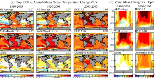
Submarine ice shelves around Antarctica and Greenland extend to ocean depths of 1 km and deeper (Rignot and Jacobs, 2002). Figure 7b shows simulated zonal mean

15

ocean temperature change versus depth for the past century and the 21st century. De-spite near absence of surface warming in the Antarctic Circumpolar Current, warming of a few tenths of a degree is found at depths from a few hundred to 1500 m, consis-tent with observations in the past half-century (Gille, 2002; Aoki et al., 2003). Modeled warming is due to GHGs, with less warming when all forcings are included.

20

Maps of simulated temperature change for the top 1360 m of the ocean (Fig. 7a) show warming around the entire circumference of Greenland, despite cooling in the

North Atlantic. This warming at ocean depth di_ffers by about a factor of two between

the alternative and BAU scenarios, less than the factor∼4 difference in summer surface

warming over Greenland and Antarctica, consistent with the longer response time of

25

the ocean. Although we cannot easily convert temperature increase into rate of melting and sea level rise, it is apparent that the BAU scenarios pose much greater risk of large sea level rise than the alternative scenario, as discussed in Sect. 6.

Surface and submarine temperature change are also relevant to the stability of

(25)

ACPD

6, 12549–12610, 2006

climate

J. Hansen et al.

Title Page

Tables Figures

◭ ◮

Back Close

Full Screen / Esc

methane hydrates in permafrost and in ocean sediments. Recent warming is already beginning to cause release of methane from thawing permafrost in Siberia (Walter et al., 2006; Zimov et al., 2006), but this methane release is not yet large enough to yield

an overall increase of atmospheric CH4, as shown in Sect. 5. Projected 21st century

summer warming in the Northern Hemisphere permafrost regions is typically a factor of

5

five larger in BAU scenarios than in the alternative scenario (Fig. 4), suggesting that the threat of a significant positive climate feedback is much greater in the BAU scenarios.

Methane hydrates in ocean sediments are an even larger potential source of methane emissions (Archer, 2006). It is possible that much of the temperature rise

in extreme global warming events, such as the approximately 6◦C that occurred at

10

the Paleocene-Eocene boundary about 55 million years ago (Bowen et al., 2006), re-sulted from catastrophic release of methane from methane hydrates in ocean sedi-ments. It may require many centuries for ocean warming to substantially impact these methane hydrates (Archer, 2006). Calculations of global warming enhancement from

methane hydrates based on diffusive or upwelling-diffusion ocean models suggest that

15

the methane hydrate feedback is small on the century time scale (Harvey and Huang, 1995). However, the positive thermal anomalies that we simulate with our dynamic ocean model at great ocean depths at high latitudes (Fig. 7) are much larger near

the ocean bottom than we would obtain with diffusive mixing of anomalies (as in our

Q-flux model), suggesting that further attention to the possibility of methane hydrate

20

release is warranted. With our present lack of understanding, we can perhaps only say with reasonable confidence that the chance of significant methane hydrate feedback is greater with BAU scenarios than with the alternative scenario, and that empirical ev-idence from prior interglacial periods suggests that large methane hydrate release is unlikely if global warming is kept within the range of recent interglacial periods.

25

(26)

ACPD

6, 12549–12610, 2006

climate

J. Hansen et al.

Title Page

Tables Figures

◭ ◮

Back Close

Full Screen / Esc

Interactive Discussion 5 Actual GHG trends versus scenarios

Global and regional climate changes simulated for IPCC scenarios in the 21st century are large in comparison with observed climate variations in the 20th century. This raises the question: is it plausible for global climate forcing to follow a path with a smaller forcing than those in the IPCC scenarios?

5

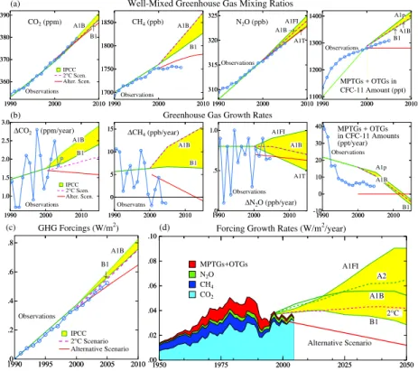
5.1 Ambient GHG amounts

Figure 8a compares GHG scenarios and observations, the latter being an update of

Hansen and Sato (2004) (seehttp://data.giss.nasa.gov/modelforce/ghgases/), who

de-fine the data sources and methods of obtaining global means from station measure-ments. Figure 8b shows the corresponding annual growth rates. Figure 8c and d

10

compare observed climate forcings and their growth rates with the IPCC, 2◦C, and

alternative scenarios.

Observed CO₂ falls close to all scenarios, which do not differ much in early years

of the 21st century. CO2 has large year-to-year variations in its growth rate due to

variations in terrestrial and ocean sinks, as well as biomass burning and fossil fuel

15

sources. However, we are able to draw conclusions in Sect. 5.3 about the realism of

CO₂scenarios by comparing emission scenarios with real world data on fossil fuel CO₂

emission trends, for which there are reasonably accurate data.

Overall, growth rates of the well-mixed non-CO2 forcings fall below IPCC scenarios

(Fig. 8a, b). Growth of CH₄ falls below any IPCC scenario and even below the

alter-20

native scenario. Observed N2O falls slightly below all scenarios. The sum of MPTGs

(Montreal Protocol Trace Gases) and OTGs (Other Trace Gases) falls between the IPCC scenarios and the alternative scenario (which was defined at a later time than the IPCC scenarios, when more observational data were available). The estimated forcing by MPTGs is based on measurements of 10 of these gases, as delineated by Hansen

25

and Sato (2004), all of which are growing more slowly than in the IPCC scenarios, with the few significant unmeasured MPTGs assumed to follow the lowest IPCC scenario.

(27)

ACPD

6, 12549–12610, 2006

climate

J. Hansen et al.

Title Page

Tables Figures

◭ ◮

Back Close

Full Screen / Esc

OTGs with reported data include HFC-134a and SF₆, for which measurements are

close to or slightly below IPCC scenarios.

Figures 8c and d show that the net forcing by well-mixed GHGs for the past few years has been following a course close to that of the alternative scenario. However, it should not be assumed that forcings will remain close to the alternative scenario,

5

because, as shown below, fossil fuel CO2emissions now substantially exceed those in

the alternative scenario.

The alternative scenario was defined (Hansen et al., 2000) as a potential goal under

the assumption of concerted global efforts to simultaneously (1) reduce air pollution (for

human health, climate and other reasons), and (2) stabilize CO₂emissions initially and

10

begin to achieve significant emission reductions before mid-century, such that added

CO2 forcing is held to ∼1 W/m

2

in 50 years and ∼1.5 W/m2 in 100 years. Thus the

alternative scenario assumes that CH4 amount will peak within a decade and then

decline enough to balance continued growth of N₂O. It also assumes that the decline

of CH4and other O3precursors will decrease tropospheric O3 enough to balance the

15

small increase in forcing (several hundredths of a W/m2) expected due to recovery of

halogen-induced stratospheric O3depletion.

The most demanding requirement of the alternative scenario is that added CO2

forc-ing be held to∼1 W/m2in 50 years and ∼1.5 W/m2in 100 years. The scenario in our

present climate simulations, for example, has annual mean CO₂growth of 1.7 ppm/year

20

at the end of the 20th century declining to 1.3 ppm/year by 2050. The plausibility of the

alternative scenario thus depends critically upon fossil fuel CO2emissions.

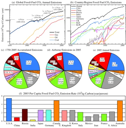
5.2 Fossil Fuel CO2emissions

Global fossil fuel CO₂emissionschange by only a few percent per year and are known

with sufficient accuracy that we can draw conclusions related to atmospheric CO2

25

trends, despite large year-to-year variability in atmospheric CO2 growth. In recent

decades the increase of atmospheric CO₂, averaged over several years, has been