A Work Project, presented as part of the requirements for the Award of a Masters Degree in Economics from the NOVA – School of Business and Economics and Maastricht University
School of Business and Economics
Social Impact of Abortion’s
Decriminalization in Portugal
*
António Melo
Nova SBE Number: 842
Maastricht SBE Number: I6123338
A project carried on the Master‚s in Economics Program under the supervision of: Professor Susana Peralta
Professor Kristof Bosmans
I dedicate this thesis to my dad.
Lisbon, 28
thMay, 2017
*I am deeply grateful to my two advisers, Susana Peralta and Kristof Bosmans for helping me to overcome the
challenges this thesis has posed. I would also like to thank the General Health Directorate -Direcção Geral da Saúdeand the National Institute of Statistics -Instituto Nacional de Estatísticafor making available individual data
on abortions and births, respectively. Also I would like to give a special thank to the General Health Directorate
Abstract
This paper studies the impact of legalizing abortion in Portugal on fertility and on maternal-infant health indicators, namely on low birth weight (LBW). It used individual-level data on all pregnancies in Portugal from 2008 to 2014. It retrieved the socio-economic determinants of abortion in Portugal to find that young women, educated, employed, working in low skilled jobs, single, with previous children, without easy access to abortion services and living in conservative regions are more prone to abort. It also found that abortion induces positive selection effects regarding LBW and that it caused a reduction in Portuguese fertility.
Keywords: Social-economic determinants of abortion; Selection effects; Fertility; Birth Out-comes
1
Introduction
In Portugal, in 2007, the voluntary interruption of pregnancy up to the tenth week of pregnancy on women´s demand was legalized by a national referendum. This legal change enlarged the spectrum of pregnancies eligible for interruption as previous legislation already allowed abortion for medical or criminal reasons.
The debate before the referendum was very intense in the Portuguese society, due to differences in ethical, religious, political and rights perspectives. The health authorities have monitored in detail the abortion implementation generating an extensive source of data and yearly descriptive reports. There is however a knowledge gap regarding the impact of induced abortion on social outcomes.
This study aims to shed light on this matter by researching two main topics related to social impact of abortion legalization. The first, to determine the impact of decriminalizing abortion on Portuguese fertility, an important epidemiology question that has so far been unanswered in the Portuguese case. The second, to estimate how birth outcomes were affected by this change in the law. More specifically we focus on the birth outcomes of gestational length and birth weight, which is considered a strong predictor of the health of the newborn.1
Both topics have been subject of great discussion in the academic literature, mainly in the United States (US), where a vast range of studies has been produced regarding the outcomes of abortion legislation and about these two outcomes in particular.
There are two main perspectives in the academic literature regarding the mechanism through which abortion legalization impacts social outcomes.
One argues that the impact of abortion in social outcomes results from birth cohort size reductions. If birth cohorts are smaller with abortion’s legalization then post-legal cohorts will represent smaller shares of the overall population, thus having a smaller weight on the population’s social outcomes. There is evidence that supports this perspective, namely, Levine et al. (1999) showed there was a fertility drop of 5% in the United States due to abortion’s legalization. This effect is commonly referred in the literature as cohort size reduction.
1Gestational length is the amount of time a pregnancy lasts.
The other main perspective is that abortion’s legalization outcomes are not only a consequence of smaller birth cohorts, but also a consequence of a different composition of birth cohorts, once abortion is made legal (Donohue and Levitt 2001). The logic behind this idea is that legal abortion reduces the number of unwanted births. Considering that unwanted children live in worse environments (Gruber, Levine, and Staiger1999), cohorts born after abortion legalization are expected to have better outcomes in several areas such as education (Pop-Eleches2006) and criminality (Donohue and Levitt2001). In the literature, this effect is commonly referred as the selection effect.
2
Previous work on abortion’s social outcomes
Several scholars have described the socioeconomic characteristics that are more frequent among women who perform induced abortions, namely: age, education level, marital status, race of the women, number of previous children, urban-rural residence, economic situation, unemployment, nationality and religion of the woman.
Sequential descriptive studies based on surveys performed by the Guttmatcher Institute in the US (Jones, Darroch, and Henshaw2002; Jones, Finer, and Singh2010; Jerman, Jones, and Onda 2016) showed that abortion is more frequent among women in their 20s,high school graduates, non-married, non-white, with at least one previous child, with metropolitan residence, poor, and with religious affiliation.
Some authors studied which socioeconomic variables lead to abortion through the usage of probabilistic models in order to determine the outcome of a pregnancy.
The following determinants have been shown to consistently increase the odds of choosing to abort: Age [in young women (Rasch et al.2008; Gius2007) and in women older than 40 years old (Rasch et al. 2008)]; Distance to abortion provider [in metropolitan women (Powell-Griner and Trent 1987; Gius 2007) as they have more access to abortion services], Cohabitation [in single women (Powell-Griner and Trent1987; Gius2007; Rasch et al.2008)], Parity [in women having children (Skjeldestad et al. 1994; Rasch et al. 2008)], Labor Market Status [in students and women in precarious labor market situation (Rasch et al.2008)]. The only determinant that was not entirely consistent across the literature was education, where Powell-Griner and Trent (1987) and Gius (2007) found that more educated women were more prone to abort contrary to Font-Ribera et al. (2008) who found that it was less educated women who had higher likelihood of abortion instead.
Moreover, there is extensive academic literature regarding abortion’s legal status and its impact on fertility and other social outcomes. Levine et al. (1999) implemented a Difference-in-Differences (DD) estimation using the different dates of abortion legalization across the US states as a natural experiment. They showed that the fertility rate dropped 5% for all women between the age of 15 and 44 years old, followed by a full rebound once abortion was legal in all states. Teenagers had a 13% decrease in birth rates. The use of this natural experiment allowed to exclude ongoing fertility trends and to precisely estimate the impact of abortion’s legalization on American fertility.
More studies reached similar findings. Levine and Staiger (2004) estimated that liberal abortion laws yielded between 9% to 17% decreases in fertility in Eastern European countries by using the countries’ legal status of abortion. Pop-Eleches (2010)found a 30% decrease in fertility and a reduction of 25% of life-time fertility in Romania after a ban of restrictive abortion laws.2
Nevertheless, the negative impact on fertility as a consequence of more permissive abortion laws is not consensual in the literature. Levine, Trainor, and Zimmerman (1996) results showed that imposing restrictions on the access to abortion had a neutral or negative impact on births and a reduction of the abortion rate.3 Kane and Staiger (1996) also found that increase in abortion restrictions decreased in-wedlock birth rates. The economic decision that women make is, therefore, an ambiguous one, with abortion legalization and implementation of abortion restrictions yielding similar effects on birth (Levine et al.1999).
Regarding selection, Gruber, Levine, and Staiger (1999) found that, using the quasi-experiment design proposed by Levine et al. (1999), the "marginal child" (defined by the authors as being the child that was not born after the legalization but would have if abortion was not available) was more likely to have lived in a worse environment compared to children on average, more precisely "60 percent more likely to live in a single-parent household, 50 percent more likely to live in poverty, 45 percent more likely to be in a household collecting welfare, and 40 percent more likely to die during the first year of life".4
Donohue and Levitt (2001) use a 20 year lag of the abortion rate as a proxy for unwanted births to conclude that abortion legalization was responsible for half of the decrease in criminality experienced in the US in the 90s. The base argument is that a great proportion of the children that are aborted would have had higher chances of entering in criminal activities and therefore abortion would affect criminality "15-20 years later when the cohorts born in the wake of liberalized abortion would start reaching their high-crime years"5This result was later challenged by Joyce (2004) who obtained a smaller impact using Levine et al. (1999) DD strategy. He argued that using the abortion rate was not an accurate measure of unwanted births since "abortion is endogenous to sexual activity, contraception and fertility" and thus "some pregnancies that were aborted in the mid- to late 1970s may not have been conceived had abortion remained illegal".6,7 In order to solve the miss-estimation of selection effects that results from both Donohue and Levitt (2001) and Joyce (2004) methodologies Ananat et al. (2009) propose an Instrumental Variables (IV’s) application that combines the DD estimation with measures of social costs of aborting, namely the level of conservatism in a state and pre-legal abortion levels, to capture
2Romania had one of the most liberal abortions policies in the world until 1966, the year after Ceausescu took
power. One of his first measures was to ban abortion which was, at the time, the main contraception method used in the Country. In 1989, after the fall of Ceausescu, the abortion ban was reversed (Pop-Eleches2010).
3The abortion rate is defined as the number of abortions per one thousand fertile women. 4Gruber, Levine, and Staiger (1999, p. 265).
5Donohue and Levitt (2001, p. 381).
6Joyce (2004, p. 2).
7Donohue and Levitt (2004, p. 47) admitted the limitations of their measure of unwanted births but counter-argued that it is a "better proxy for the impact of legal abortion" then the DD which is insufficient to capture the impact of abortions since it considers that abortion legalization alone makes abortion equally accessible to all woman, disregarding "costs (financial, social, and psychological) of abortion across time and place".
where illegal abortion demand was higher, assuming that states with high demand for illegal abortion have lower latent costs. Regarding crime, the authors concluded that the reduction was a consequence of smaller cohorts and not due selection effects.8.9
Joyce (1985) concluded that abortion culminates in less unwanted births which in turn result in healthier children. Grossman and Joyce (1990) confirmed this using data on birth weights of black mothers from New York. Currie, Nixon, and Cole (1996) on the other hand found that abortion restrictions appear to have no significant impact on birth-weight or on birth-weight distribution, which might indicate that there is no selection effect.
3
The Portuguese Case Context
3.1
Evolution of abortion’s legal framework
Induced abortion was illegal in Portugal until 1984, when a new law allowed pregnancy to be interrupted up to 12 weeks of gestation in cases where the pregnancy represented a threat to the woman’s life or could cause long-term physical or mental health damage, and in cases where the pregnancy resulted from a crime against sexual freedom (Lei 6/84). In the case where there had occurred fetal malformations, abortion was available until 16 completed weeks of pregnancy. Subsequent revisions of the law changed the threshold for crimes against sexual freedom to 16 weeks (1994) and fetal malformation to 24 weeks (1997). Thereafter, two referenda took place, in 1998 and 2007. Both on the same question:
Do you agree with voluntary interruption of pregnancy’s decriminalization if per-formed by the woman’s will until 10 weeks in a previously legally authorized health center?
In the first scrutiny "No" won with 50.07% of the votes and an abstention rate of 68.11%.10 Consequently the law suffered no changes. In the second one "Yes" won with 59,25% and a abstention rate of 56.43%.11 The new law allowed abortions on woman’s demand until 10 completed weeks of pregnancy. The law also required a three days reflection period before the final decision of aborting. The law was enacted on the 15th of July of 2007 (Lei 16/07).12 It
is important to note that although the law was implemented nationwide, the autonomous region of Madeira only put the law into effect on the 1stof January of 2008 with a six month delay in
8Interestingly, they found positive selection effects for other social outcomes, namely: single parenthood, receiving
welfare and graduating college. These findings are coherent with the theory of positive selection, since "the marginal birth is 23% to 69% more likely to be a single parent, 73% to 194% more likely to receive welfare, and 12% to 31% less likely to graduate college" (Ananat et al.2009, p. 135).
9Pop-Eleches (2006) too has provided evidence regarding negative selection regarding education outcomes and crime in Romania.
10CNE. 2017a.Resultados Eleitorais.URL:http://eleicoes.cne.pt/raster/index.cfm?dia=28&mes=06& ano=1998&eleicao=re1.
11CNE. 2017b.Resultados Eleitorais.URL:http://eleicoes.cne.pt/raster/index.cfm?dia=11&mes= 02&ano=2007&eleicao=re1.
12Although the participation rate of the referendum was not high enough to be binding, because turnout was below
50%, the government chose to change the law, since in its eyes it was the expressed will of the people (Alves et al.
2009).
relation to the rest of the country. During six months the only way for women of the archipelago to get a legal abortion was to travel to the mainland, without any financial aid from the regional government, and perform it there.
3.2
Brief overview of illegal abortion prior to legalization
Dias and Falcão (2000) estimated that in the 90s Portugal had around 20 000 illegal abortions per year.13 For the year of 2004 the WHO reported an estimate of 24 000. The Family Planning Association - Associação para o Planeamento da Família presented a similar number (19 000
illegal abortions) in their report of 2006. The report based on a randomized survey to 2000 women allover Portugal, of which 270 had made an abortion. Abortions were predominantly performed in private houses (39.4%) or private clinics (32.2%) and the most prevalent method wassurgical.
The majority of women did not graduate school and 27.4% reported having complications (APF 2006).
Illegal abortion was a cause of maternal morbidity and mortality. At least 14 women died due to post-abortive complications between 2002 and 2007, a lower-bound estimation (DGS 2009). With legalization abortion complications decreased, thus allowing an improvement of public health.14
3.3
Fertility trends
In 1960 Portugal had a total fertility rate of 3.2 live births per woman in fertile age with the first child born, on average, at the age of 25.15 Since then Portuguese fertility has had a gradual decline, to reach the lowest fertility rate in EU-28 countries, of 1.23 versus an average of 1.58, with an increase of 5 years in the mean age at first child (Valente Rosa2010).16,17
Nevertheless, the infant mortality has evolved in the opposite direction of the population renewal and was of 2.8 dead infants per 1000 live births in 2014, below the 3.7 infant mortality rate average of the EU28 (DGS 2015). This figures reflects not only the improvement of social conditions during the last three decades of the 20th century, but also a substantial effort of the National Health System that implemented a Maternal and Infant Health surveillance programs and a comprehensive national vaccination plan (Valente Rosa2010).
13This number was obtained using number of emergency room visits due to abortion complications to which the
authors apply a multiplier to get the overall number.
14Although legal abortion shows a decreasing trend and has substantially replaced illegal abortion, we estimate
that illegal abortion still occurs at a residual percentage (Appendix A). This matter deserves a critical reflection on access equity.
15Total fertility rate is defined as being the number of births per fertile woman.
16From PORDATA: http://www.pordata.pt/Portugal/Idade+m%C3%A9dia+da+m%C3%A3e+ao+ nascimento+do+primeiro+filho-805
17 From Eurostat: http://ec.europa.eu/eurostat/statistics-explained/index.php/Fertility_ statistics#Source_data_for_tables_and_figures_.28MS_Excel.29
3.4
Birth Weight and Prematurity: trends and drivers
Low birth weight (LBW) has been defined by the World Health Organization (UNICEF and WHO2004) as weight at birth below 2,500 grams. LBW is recognized as a strong predictor of health because it increases the vulnerability to foetal and neonatal mortality (20 times increase and morbidity, to limitation of growth and development, to lifetime chronic diseases and to future LBW pregnancies (WHO 2015).18 LBW results from maternal malnutrition, maternal arterial hypertension, multiple births, teenage pregnancy, inadequate rest and continued hard work during pregnancy, stress, anxiety and other psychological factors, smoking during pregnancy and exposure to second-hand smoke, acute and chronic infection during pregnancy and prematurity (UNICEF2002).19
On the other hand, newborns with high birth weight or large for gestational age (LGA) are also at risk. LGA is arbitrarily defined as a birth weight higher than 4000 g irrespective of gestational age (or above the 90thpercentile for gestational age) (Zamorski and Biggs2001). This situation has also been identified as a risk for perinatal and maternal complications, but also for the newborn future health (cancer and obesity) and development. Diabetes and maternal obesity are known causes of LGA (Das 2004), other potential causes with less clear influence have been identified in the literature as multiparity (having more than one child), advanced maternal age, ethnicity, excessive weight gain, marital status, smoking, prolonged labour (Ng et al. 2010). In 2010, Webb (2014) analyzed the relationship between socio-economic status and high birth weight and suggested that high socio-economic status does lower the risk of LGA.
The WHO defines prematurity as being born before 37 weeks of gestation (WHO 2015). Preterm birth might result from risk factors as multiple pregnancies, maternal infections and chronic conditions (diabetes and hypertension) but according to WHO in most cases a cause can not be identifiable. Most of these babies survive due to the health care provided during pregnancy, delivery and postnatal period (Barros, Clode, and Graça2016). 20,21
3.5
Data Sources and descriptive statistics
Data on abortions were provided by General Health Directorate -Direcção Geral da Saúde(DGS).
The database comprises individual information about women who aborted in Portugal from 2008 until 2014.22 This data is collected through a survey which hospitals are legally required to run on women who perform abortions and that afterwards must be reported to the Portuguese authorities.
18Can lead to chronic diseases such as type 2 diabetes, hypertension and cardiovascular disease.
19According to WHO (2010) (in an assessment of the Portuguese Health System), the rate of low birth weight infants in Portugal in 2008 was 7.7% and has increased compared to the previous 10 years period (7.1% in 2000), reaching one of the highest values of the EU15. The rise of the proportion of migrant mothers is one of the proposed explanations.
20Over the last four to five decades, Portugal has developed strategies to enhance existing prenatal care services and has a very comprehensive pregnancy health surveillance program that promotes the screening and management of pregnancy risks and risky pregnancies, and a very efficient network of perinatal hospital care.
21Prematurity has shown the same trend of LBW, which has been increasing over time from 5.5% of all births in
2001 to 8.7% in 2009, according to the Portuguese Authorities (ACS and INSPA2010).
22Data from 2007 was not provided by DGS.
This survey contains socioeconomic variables from which the most relevant for this study are the municipality of residence of the woman, the date of the abortion, the education of the woman, the working condition of the woman, the marital status, the education and working condition of the partner, number of children and number of pregnancies. In Portugal, DGS publishes every year, since 2008, a descriptive report of the abortion situation in Portugal based on the data collected through a mandatory survey at a national level. Since it was legalized, abortion has steadily been more frequent among women between 20 and 34 years old, women that graduated high-school, women with no children and with no previous abortions, unemployed, students, non-qualified, agricultural and manufacturing workers. Approximately half of the women who abort live with their partner.
Data on births was provided on request by the National Institute of Statistics - Instituto
Nacional de Estatística(INE) from 2002 until 2015. It comprises variables that are also present
on the abortion database, thus forming a homogenized data-set for all pregnancies in Portugal from 2008 until 2014.
Data for municipal monthly insured unemployment were retrieved from the Institute for Professional Development and Employment - Instituto do Emprego e Formação Profissional
monthly reports on municipal unemployment published every month since January of 2004 and from the Institute for Employment of Madeira -Instituto de Emprego da Madeiramonthly reports
on municipal unemployment published every month since January of 2006.
The referendum results of each municipality were retrieved from the General Economic Activities Directorate -Direção-Geral das Atividades Económicaswebsite.
The demographic and social characteristics of the studied population of women who gave birth or aborted in Portugal from 2008 to 2014 are summarized in Table 1. There was a total of 623,440 births and 130,735 abortions in Continental Portugal during this time period. Despite the existence of more data on births, due to the fact that there are only data on abortions from 2008 until 2014, we restricted the data sample to this period in order to have a comparable data-set between births and abortions.
Some interesting patterns emerge from Table 1: Women younger than 24 represent higher shares of abortions than births, while those aged between 25 and 39 have the opposite pattern; There is an education and labor market status gradient both of the woman and the partner in the probability to abort; Women living with partners represent a higher share of births than single women but a very similar share of abortions; Women with previous children only represent 9% of the share of births, contrasting with a 60% share regarding abortions.
Table 2 comprises summary statistics of the municipalities included in the municipality-level regression analysis. ´
Table 1: Demographic and social characteristics of the study population - Descriptive Statistics
Births Abortions Pregnancies
SD N % N % N %
Age Group Less than 24 y.o .406
- <20 23,036 3.69% 14,861 11.37% 37,897 5.02% - 20-24 75,858 12.17% 28,884 22.09% 104,742 13.89% More than 25 and less than 39 y.o .430
- 25-29 159,793 25.63% 28,162 21.54% 187,955 24.92% - 30-34 217,498 34.89% 27,244 20.84% 244,742 32.45% - 35-39 121,364 19.47% 21,819 16.69% 143,183 18.99% More than 40 y.o .186
- 40-44 23,724 3.81% 8,871 6.79% 32,595 4.32% - >45 2,167 0.35% 894 0.68% 3,061 0.41%
100% 100% 100%
Education Less than 12 years of schooling .499
- Basic (<12 years) .499 238,544 38.26% 59,676 45.65% 298,220 39.54% More than 12 years of schooling .499
- High school (>12 & <15 years) .442 180,234 28.91% 44,907 34.35% 225,141 29.85% - College (>15 years) .439 204,662 32.83% 26,152 20.00% 230,814 30.60%
100% 100% 100%
Work Status Unemployed .458 190,708 30.59% 47,706 36.49% 238,414 31.61%
Employed .458 432,732 69.41% 83,029 63.51% 515,761 68.39%
100% 100% 100%
- Educational Intensive .371 118,825 27.46% 11,581 13.95% 130,406 25.28% - Educational Medium-Intensive .499 271,707 62.79% 44,682 53.81% 316,389 61.34% - Educational Non-Intensive .266 42,200 9.75% 26,766 32.24% 68,966 13.37%
Cohabitation Without Partner .316 68,676 11.02% 64,413 49.27% 133,089 17.65% With Partner .316 554,764 88.98% 66,322 50.73% 621,086 82.35%
100% 100% 100%
Unemployed Partner .261 66,663 12.02% 9,563 14.42% 76,226 12.27% Employed Partner .261 488,101 87.98% 56,759 85.58% 544,860 87.73%
100% 100% 100%
- Educational Intensive .360 113,026 23.16% 7,540 13.28% 120,566 22.13% - Educational Medium-Intensive .490 324,574 66.50% 37,080 65.33% 361,654 66.38% - Educational Non-Intensive .240 50,501 10.35% 12,139 21.39% 62,640 11.50%
Parity No children .325 566,749 90.91% 52,678 40.29% 619,427 82.13%
With children .325 56,691 9.09% 78,718 59.71% 134,748 17.87%
100% 100% 100%
- One child .257 38,478 67.87% 38,718 49.60% 77,196 57.29% - Two children .184 13,350 23.55% 28,880 37.00% 42,230 31.34% - More than three children .116 4,863 8.58% 10,459 13.40% 15,322 11.37%
Total 623,440 100% 130,735 100% 754,175 100%
SD Mean
Distance to abortion Provider (100Km) .158 .107
% of Yes votes in Referendum 16.97 60.03
Note: These descriptive statistics only include data from Continental Portugal between 2008 and 2014 as well as logistic regressions. This happens because there is no data for distance to nearest abortion provider for Madeira and the Azores (since these regions are islands, the variable distance would not be comparable between Continental Portugal and Madeira and the Azores).
Table 2: Descriptive Statistics of variables included in regressions using monthly municipal-level data
Reg. using legal status Distance as IV Beja Diff-in-Diff as IV
Mean SD Mean SD Mean SD Mean SD Mean SD Mean SD
(Overall) (Within Munic.) (Overall) (Within Munic.) (Overall) (Within Munic.)
Birth rate (Overall) 2.91 1.25 3.02 1.11 2.80 1.23 3.02 1.10 2.87 1.72 2.94 1.58
Birth rate (<24 y.o) 2.34 2.19 2.55 2.01 2.08 2.11 2.55 2.01 2.57 3.19 2.86 3.07
Birth rate (>25 & <39 y.o) 5.10 2.37 5.18 2.09 5.03 2.38 5.19 2.08 4.93 3.26 4.89 3.05
LBW Incidence (Overall) 7.85 11.82 7.23 10.06 8.15 12.37 7.27 10.09 7.76 16.15 6.99 14.54
LBW Incidence (<24 y.o) 5.88 15.94 5.74 14.57 5.73 16.15 5.79 14.65 4.88 17.64 4.62 16.48
LBW Incidence (>25 & <39 y.o) 7.49 12.73 6.88 11.01 7.76 13.20 6.91 11.03 7.42 17.44 6.35 15.02
LGA Incidence (Overall) 3.90 8.54 3.97 7.32 3.77 8.71 3.95 7.27 3.74 12.10 4.07 11.41
LGA Incidence (<24 y.o) 2.68 10.90 2.78 9.97 2.48 10.70 2.76 9.93 1.60 10.54 2.11 11.09
LGA Incidence (>25 & <39 y.o) 3.91 9.36 4.02 8.29 3.76 9.33 4.00 8.23 3.82 12.85 3.93 12.05
Prem. Incidence (Overall) 7.37 11.70 6.62 9.88 7.52 11.94 6.68 9.89 6.14 14.00 5.84 13.21
Prem. Incidence (<24 y.o) 5.32 15.34 4.99 13.67 5.04 15.35 5.06 13.81 3.94 16.40 3.85 14.86
Prem. Incidence (>25 & <39 y.o) 7.22 12.79 6.46 10.94 7.41 13.00 6.51 10.93 5.83 14.95 5.49 14.21
Unemploymentper capita 0.07 0.03 0.07 0.02 0.08 0.03 0.07 0.02 0.08 0.02 0.08 0.02
Abortion rate (Overall) 0.47 0.51 0.40 0.41 0.56 0.77 0.44 0.62
Abortion rate (<24 y.o) 0.66 1.12 0.54 0.90 0.69 1.55 0.53 1.27
Abortion rate (>25 & <39 y.o) 0.62 0.83 0.51 0.68 0.78 1.32 0.58 1.06
Distance to nearest provider 27.36 22.39 27.36 3.42 46.32 30.72 47.69 13.45
Observations 37.884 23.352 1.392
4
Birth outcomes as evidence of selection
4.1
Socio-economic determinants of abortion
In order to find the determinants of abortion in Portugal, a probit model was used, represented in the equation below:
Pr(Birt hi)= φ(βXi+αCmi+εi) (1)
Where φ is the cumulative distribution function of the normal distribution, the dependent variable is Birt hi which is a birth (binary) indicator, Xi is a vector of the individual controls:
AgeGr oupiis a categorized variable of the age of the woman (teenagers, women aged between 20
and 34 years old and women older than 35 years old),E ducationLeveliis a categorized variable
of the woman’s education level (basic education, high school and college), Partneri indicates
if woman has partner,Unemployedi andUnemployedPartneri are indicators of the woman or
partner’s joblessness,JobTypeiandPartner sJobTypei are categorized variables of the woman
or partner’s labor market status(high educational intensive jobs, medium educational intensive jobs and educational non-intensive jobs) Number o f Childr eni is a categorized variable of the
number of children a woman has (one, two or more than three children). Cmi is a vector which
captures the social environment where the woman lives comprised by: Distancei, a variable
that measures the distance between the town hall of a woman’s municipality to the town hall of the nearest municipality with an abortion provider,Y esV oteW oniwhich indicates if in the 2007
referendum the vote "Yes" won in the woman’s municipality andE ducationLeveli×Y esV oteW oni
which interacts the educational level of the woman with the direction of the vote of the woman’s municipality in the 2007 referendum.
We follow Levine et al. (1999) and divide the woman’s age groups into 3 categories, based on whether the share of total abortions is greater than the share of total births. The age categories we used are the following: Women younger than 24 years old, woman aged between 25 years old and 39 years old and women older than 40 years old.23
Table 3 displays three different probit models. Columns 1 presents a probit model where education is represent by two variables, having less than 12 years of schooling (the default variable) and having more than 12 years of schooling. Regarding Work Status, the regression in column 1 only analysis whether the woman and the partner are unemployed, disregarding the type of job they perform. Finally, variable Yes is a variable that indicates whether the Yes vote won in the referendum of 2007. Column 2 in-depths our analysis by dividing the Education category in three levels: having basic schooling (less than 12 years of education), having high school (more than 12 years of education but less than 15) and having college (more than 15 years of education). The analysis of Work status both for the woman and partner not only considers whether they are unemployed (as column 1), but also, in the case they are employed, what type of job are they
23Levine et al. (1999) uses the following age categories: women younger than 20, women aged between 20 and
34 and women aged between 35 and 49.
performing. As for the variable that relates the referendum results to the probability of having an abortion, instead of treating the yes vote as a dummy variable as in column 1, this regression uses the percentage of yes votes in the woman’s municipality. All other variables of column 2 are present in column 1. Column 3 is similar to column 2 with the difference that the referendum variable being used is the same as in column 1.
The results in column 3 of Table 3 show that women younger than 24 years old, who are employed, who work in poorly differentiated jobs, who are educated, with no cohabitation, with easy access to abortion providers and living in pro-abortion areas are more prone to abort.24 In what concerns the influence of the level of education on the probability to abort, these results are in accordance with Powell-Griner and Trent (1987)and Gius (2007), however they are discrepant with Font-Ribera et al. (2008), who concluded that low educated women were more vulnerable. With respect to cohabitation, these results are aligned with Powell-Griner and Trent (1987), Skjeldestad et al. (1994) and Rasch et al. (2008). Regarding the number of children our results are coherent with the results of Skjeldestad et al. (1994), finding that the probability of choosing abortion increases with parity. As for the distance to abortion provider, our results are consistent with the studies that showed that metropolitan women are more prone to abort, since abortion centers are concentrated in metropolitan areas, and therefore non-metropolitan areas are farther away from abortion centers (Jones, Darroch, and Henshaw2002; Jones, Finer, and Singh2010; Jerman, Jones, and Onda2016; Powell-Griner and Trent1987). We searched the literature and we did not identify studies exploring the impact of the woman’s or partners employment status or job type in abortion.
It is important to highlight that these results were obtained using data on the whole population of pregnant women in Portugal in the period from 2008 to 2014. Unfortunately it was not possible to match some variables that would have added value to the analysis conducted, more specifically, it was not possible to identify in the newborns database if the women were students, how many abortions women had previously and if they went to a family planning medical appointment. The fact that we cannot identify individuals across the database also does not allow to follow the evolution of women decisions, but it would be extremely difficult to retrieve such data unless it had been collected with that purpose. It would nevertheless be interesting if such a study was performed in Portugal, since it would add more information on how Portuguese women decide across time.
4.2
Selection effects
Once the determinants of abortion in Portugal were estimated, we tested if abortion leads indeed to selection effects on birth outcomes. This was done by implementing a Heckit model.25 We
24We analise column 3 since it is the regression with the highest fit (PseudoR2of 0.4238).
25A procedure purposed in Heckman, James. 1979. "Sample Selection Bias as a Specification Error." Economet-rica. 47 (1): 153-162
Table 3:The determinants of Abortion in Portugal: Logistic regressions
Giving Birth
(1) (2) (3)
Age 0.338∗∗∗ 0.340∗∗∗ 0.340∗∗∗
(0.00275) (0.00287) (0.00287)
Age Squared -0.00485∗∗∗ -0.00475∗∗∗ -0.00475∗∗∗
(0.0000458) (0.0000480) (0.0000480)
At least High school (> 12 years) -0.378∗∗∗
(0.00987)
- High school (> 12 and <15 years) -0.403∗∗∗ -0.445∗∗∗
(0.0106) (0.0117)
- College (> 15 years) -0.706∗∗∗ -0.750∗∗∗
(0.0120) (0.0131)
Unemployed 0.301∗∗∗ 0.192∗∗∗ 0.192∗∗∗
(0.00552) (0.00603) (0.00603)
- Education Intensive Job 0.122∗∗∗ 0.123∗∗∗
(0.00808) (0.00807)
- Education Non-Intensive Job -0.553∗∗∗ -0.553∗∗∗
(0.00774) (0.00774)
With Partner 1.142∗∗∗ 1.159∗∗∗ 1.158∗∗∗
(0.00548) (0.00586) (0.00587)
Partner is unemployed -0.0572∗∗∗ -0.0549∗∗∗ -0.0539∗∗∗
(0.00795) (0.00837) (0.00837)
- Partner has Education Intensive Job 0.147∗∗∗ 0.148∗∗∗
(0.00805) (0.00805)
- Partner has Education Non-Intensive Job -0.112∗∗∗ -0.113∗∗∗
(0.00814) (0.00814)
With Children -1.966∗∗∗
(0.00554)
- 1 Child -1.682∗∗∗ -1.682∗∗∗
(0.00651) (0.00651)
- 2 Children -2.433∗∗∗ -2.433∗∗∗
(0.00896) (0.00896)
- More than 3 Children -2.537∗∗∗ -2.536∗∗∗
(0.0137) (0.0137)
Distance to nearest abortion provider (100Km) 0.357∗∗∗ 0.392∗∗∗ 0.379∗∗∗
(0.0146) (0.0150) (0.0150)
Yes vote won -0.125∗∗∗ -0.112∗∗∗
(0.00840) (0.00876)
- Percentage of Yes votes -0.00191∗∗∗
(0.000192)
At least High School x Yes vote won -0.0569∗∗∗
(0.0109)
- High School x Yes vote won -0.143∗∗∗ -0.0894∗∗∗
(0.0113) (0.0130)
- College x Yes vote won -0.121∗∗∗ -0.0633∗∗∗
(0.0116) (0.0134)
Observations 752579 752579 752579
PseudoR2 0.3953 0.4237 0.4238
Marginal effects; Standard errors in parentheses (d) for discrete change of dummy variable from 0 to 1
∗p<0.10,∗∗p<0.05,∗∗∗p<0.01
chose this method since it enables to account for the truncation of our data and to test if there is selection.26
In our paper we are in the presence of a typical selection problem. We aim to understand, depending on the woman’s socio-economic profile and her propensity to abort, how birth outcomes vary among the population. This situation is depicted by equation 2.
yi = xi′β+ε with ε∼ N (0, σ
2
) (2)
The issue is that it is impossible to observe the birth outcomes of women who abort. In equation 3 we depict this problem. The selection variablezi(which indicates if the woman gave
birth) depends on the woman’s characteristics (age, education, labor market status, parity and cohabitation) as well as on her surrounding environment (distance to nearest abortion provider and level of conservatism of the municipality).
zi =w′jγ+u with u ∼ N (0,1) (3) Since we already know which variables influence the selection variable zi from our model
that estimated the socio-economic determinants of giving birth, we now perform a two stage estimation instrumenting the Inverse Mills Ratio (IMR) derived from our probit model displayed in column 3 of Table 3 on equation 2. Equation 4 below displays this process.
E(yi|ui > −w′jγ)= x′iβ+ρσε
φ(w′jγ)
Φ(w′jγ)
where ρ= corr(εi,ui) and I M R=
φ(w′jγ)
Φ(w′jγ) (4)
Using Stata’s command Hekcman (which corrects for the bias of the standard errors in models of selection), we applied linear probability regressions having as dependent (binary) variables LBW, LGA and prematurity indicators. This enables us to infer the direction of the birth outcomes of the "marginal child". In order to understand the selection’s direction we analyze the sign of ρ. If ρis negative then women who have higher likelihood of giving LBW, LGA or premature children are not giving birth. If ρis positive the contrary selection effect is observed.
The results of this regressions are in table 4. Column 1 to 3 regress all the socio-economic variables of the woman on the outcome variables. The municipalities related variables (distance to abortion center and the 2007 referendum results) were not included in the second stage regressions since these should not directly affect birth weight or gestational length.
The negative and highly significant coefficient of the IMR displayed in column 1, provides ground to infer that we are in the presence of positive selection, meaning, that women who are
26It is not possible to observe the birth outcomes of the woman who aborted.
Table 4: Birth Outcomes of the "marginal child"
LBW LGA Premature
(1) (2) (3)
Age -0.00772∗∗∗ 0.00412∗∗∗ -0.00372∗∗∗
(0.000648) (0.000438) (0.000630)
Age Squared 0.000149∗∗∗ -0.0000595∗∗∗ 0.0000854∗∗∗
(0.0000103) (0.00000699) (0.0000100) Unemployed 0.00179∗ 0.00669∗∗∗ 0.000761
(0.000944) (0.000638) (0.000916)
- Education Intensive Job -0.000423 -0.00225∗∗∗ 0.00192
(0.00123) (0.000832) (0.00120)
- Education Non-Intensive Job 0.00190 0.00888∗∗∗ 0.000305
(0.00167) (0.00113) (0.00162) - 1 Child 0.00878∗∗∗ 0.00546∗∗∗ -0.00613∗∗
(0.00270) (0.00183) (0.00263)
- 2 Children 0.0247∗∗∗ 0.00357 0.00289
(0.00455) (0.00307) (0.00442)
- More than 3 Children 0.0382∗∗∗ 0.0118∗∗∗ 0.00548
(0.00563) (0.00381) (0.00547) High school (> 12 and <15 years) -0.00438∗∗∗ -0.000788 -0.00411∗∗∗
(0.000997) (0.000673) (0.000968)
College (> 15 years) -0.00395∗∗∗ -0.00910∗∗∗ -0.00582∗∗∗
(0.00126) (0.000850) (0.00122)
With Partner -0.0274∗∗∗ 0.00891∗∗∗ -0.00443∗∗
(0.00207) (0.00140) (0.00201) Partner is unemployed 0.00400∗∗∗ -0.00128 -0.00191
(0.00126) (0.000851) (0.00122)
- Partner has Education Intensive Job -0.00263∗∗ -0.00350∗∗∗ 0.000102
(0.00111) (0.000749) (0.00108)
- Partner has Education Non-Intensive Job -0.00232 0.00192∗∗ -0.00348∗∗
(0.00142) (0.000959) (0.00138)
Inverse Mills Ratio -0.0208∗∗∗ 0.00497∗ 0.00817∗∗
(0.00385) (0.00260) (0.00374)
Observations 752579 752579 752579
WaldChi2(14) 1023.94 1100.35 613.28
Standard errors in parentheses
∗ p<0.10,∗∗p<0.05,∗∗∗ p<0.01
more prone to give birth have lower odds of giving birth to LBW children.27 The positive (and significant) IMR of columns 2 and 3 indicates that women who are more prone to give birth are more likely to have LGA or premature children, which leads to the conclusion that the abortion phenomenon results in negative selection effects regarding LGA and prematurity.
Thus these findings add new evidence that abortion does induce selection effects. They also show that both women who are more prone to give birth and women who are more prone to abort have the risk of giving birth to unhealthy children depending on the considered outcome.
5
Impact of legalizing abortion on Portuguese fertility
5.1
Regression Using Legal Status of Abortion
Moving on to the municipal-level analysis, two different methods were employed to estimate the impact of legalizing abortion in fertility. First, we used the different timing of implementation of the law between Continental Portugal and the autonomous region of Madeira. The aim of this regression is to exploit these different legislative timings in order to treat Madeira as a control group for the rest of Portugal. For this identification strategy, monthly municipal panel data on births and insured unemploymentper capitafrom 2004 until 2015 were used.28 The mathematical
expression of the legal status regression just described is the following:
ln(Birt hRatemt)= β0+ β1LawImplementationmt +contr olsmt +εmt (5)
Where Birt hRatemt is the the municipal birth rate, defined as being the monthly municipal
number of births per 1000 women. LawImplementationmt is a dummy variable that takes
the value of 1 once the law is implemented and 0 otherwise.29 The variable’s coefficient is interpreted relative to the pre-law implementation period when abortion was illegal. All variables are aggregated to the monthly (t) municipal (m) level. The controls included where time and
municipality fixed effects, and the monthly municipal insured unemployment rate per one thousand inhabitants (in order to capture non-linear effects on fertility of the socioeconomic environment of each municipality).
Table 5 shows the regressions in which the different law implementation timing was used to determine the impact of abortion on fertility in Portugal and across different age groups. Columns 1,2,4 and 6 use data from the year of 2004 until 2014 and columns 3, 5 and 7 use a narrower time window from 2006 to 2009, in order to focus on a shorter range of years around the time where abortion was made legal so that we make sure that we are not including unidentifiable exogenous variations. Consequently, we consider that regressions in columns 3, 5 and 6 are better grasp the effect of legalizing abortion on social outcomes. Column 2 includes municipality-specific trends.
27Here we consider that we are in the presence of positive selection since woman who are more prone to abort would have had children with worse outcomes and therefore, abortion leads to a selection of the population which is healthier.
28The time range is wider using this method because it does not rely on abortion data.
29The law was implemented on the 15th of July of 2007 in Continental Portugal and the autonomous region of
Azores and on the 1stof January of 2008 in the region of Madeira.
This column was introduced because it has similar controls to the regressions used in Levine et al. (1999). Nevertheless, we prefer the regressions that do not use municipality-specific trends since we already use municipality and time fixed-effects and thus, adding such a control would impose to many restrictions on our data that could neutralize the true effect of legalizing abortion on social outcomes. In columns 4 and 5 the dependent variables refer to women younger than 24 years old. In columns 6 and 7 the dependent variables refer to women aged between than 25 and 39 years old. Women older than 40 were excluded from the regression since they represent a residual proportion of both births and abortions.
Regarding the impact of legalizing abortion on fertility, based on table 5 there appears to be a neutral impact since all coefficients are not statistically significant.
Table 5: Regressions using Legal Status of Abortion
All ages Less than 24 25 to 39
(1) (2) (3) (4) (5) (6) (7)
Law Implementation 0.00539 0.0733 0.0539 0.0526 0.102 -0.0141 0.0363 (0.0497) (0.0534) (0.0515) (0.0992) (0.0967) (0.0547) (0.0545)
Observations 37884 37884 20676 37884 20676 37884 20676
F 32.58 . 13.58 25.61 8.059 19.08 8.330
Note: All regressions have municipal and time fixed-effects and include municipal unemploymentper capita. Columns 2 has municipal-level specific trends. Columns 1, 4 and 6 use data from 2004 until 2014 (the full data on births could not be used since we only have unemployment data from 2004 until 2014). Columns 3, 5 and 7 use data from 2005 until 2010.
Robust standard errors in parentheses.
∗p<0.10,∗∗ p<0.05,∗∗∗p<0.01
This first method to estimate the impact of legalizing abortion on fertility might be subject to some potential limitations such as the short time span of 6 months between the law implementation in Continental Portugal and Azores versus Madeira along with the specific characteristics of the Madeira region, with its own socioeconomic and cultural differences attributable to insularity (Barros 2011). For this reason, we will resort to another method that aims to account the endogeneity between abortion rates and birth rates through the use of Instrumental Variables.30
5.2
Instrumental Variables
We will use two different instruments separately. The procedure will be as follows:
AbortionRatemt = β0+ β1Instrumentmt+contr olsmt+εmt (6)
30As explained by Joyce (2004), abortion rates might not be capturing the variation of unwanted births as a consequence of different sexual and contraceptive behaviour across municipalities.
Then the fitted values of AbortionRatemt will be plugged into the original regression:
ln(Birt hRatemt)=α0+α1AbortionRate mt+contr olsmt +εmt (7)
5.2.1 Distance to abortion provider as an instrument
In both regressions, monthly municipal-level panel data from 2008 until 2014 are used. The first instrument corresponds to the distance to the nearest abortion provider. Thus the first stage regression will be:
AbortionRatemt = β0+β1Distancemt +contr ols+εmt (8)
Where AbortionRatemt is defined as the monthly municipal number of abortions per 1000
women between the age of 15 and 49 andDistancemt is the straight line distance in kilometers
between each municipality’s town hall and the town hall of the nearest municipality with an abortion provider (for municipalities that have abortion providers the distance is 0). All variables are aggregated to the monthly (t) municipal (m) level. The controls included where time and
municipality fixed effects, and the monthly municipal insured unemployment rate per one thousand inhabitants.
The variable distance is a valid instrument since it is both relevant and exogenous. It is relevant because the farther an abortion provider is, the higher will be the cost for women to abort(since it takes more time to reach the abortion provider and it is associated with travel costs that must be supported by the women).31 Table 6 shows that distance appears to have an impact on the number of abortions made in each municipality.
The instrument is also exogenous, since it is not expected that the birth rate is correlated with the distance to the nearest abortion provider.
In Portugal there is equity in terms of access to perinatal assistance. Even if the woman has no resources to access the health services in order to deliver birth, its the state’s obligation to assure those services take place. Therefore distance to perinatal services (which sometimes coincide with abortion services) is not a source of inequity to health access and thus should not influence the distribution of births across the country.
This exclusion restriction would not hold if abortion providers were allocated to each region based on the quality of the hospitals’ services as in that case the distance to the abortion provider would be related with health outcomes, including birth weight, and therefore demand to deliver birth would be higher in these hospitals. We contacted DGS to clarify the criteria for the national distribution of abortion centers.32 DGS replied that there was no centralized policy or rationale regarding the distribution of abortion centers and that it relied on the capability of the public hospitals to o provide abortion services according to the decision of their administration
31It is expected that longer distances reduce the incentive to abort and thus municipalities with less access should
in theory have less abortions as the results derived from Section 6.2.1 and previous studies show (Jones, Darroch, and Henshaw2002; Jones, Finer, and Singh2010; Jerman, Jones, and Onda2016; Powell-Griner and Trent1987).
32The correspondence can be found in Appendix C.
boards. This capability is strongly influenced by the availability of human resources that are not conscientious objectors. A survey conducted by health care professionals on the access to abortion services in public hospitals showed that lack of logistic resources and high number of conscientious objectors health care professionals are the main reasons for hospitals not opening or closing abortion services (Alves 2015). As a consequence, the geographical distribution of abortion centers has some component of randomness which provides grounds to be confident about the exogeneity of this instrument.
Table 6 presents the first stage regression using distance as an instrument for the abortion rate. Columns 1 and 2 have the overall abortion rate as the dependent variable, column 3 has the abortion rate of women younger than 24 years old and column 4 has the abortion rate of women aged between 25 and 39 years old as the dependent variable. Women older than 40 were excluded from the regression since they represent a residual proportion of both births and abortions. It is possible to observe that as distance increases, overall abortion rates decrease as do the abortion rates for the age specific groups. This result is in accordance with the theory that longer distances reduce the incentives to abort by rising the implicit cost of abortion.
Table 6: First stage regression using distance to nearest abortion provider as instrument of the abortion rate
All ages Less than 24 25 to 39
(1) (2) (3) (4)
Distance to nearest -0.00138∗∗∗ -0.00155∗∗∗ -0.000964∗∗ -0.00189∗∗∗
abortion provider (0.000253) (0.000445) (0.000462) (0.000367)
F statistic 29.70 12.08 4.343 26.48
F p-value 0.000 0.000 0.037 0.000
Note: All regressions have municipal and time fixed-effects and include municipal unemploymentper capita. Column 2 has municipal-level specific trends.
Robust standard errors in parentheses.
∗p<0.10,∗∗ p<0.05,∗∗∗p<0.01
Table 7 presents the second stage regression. In columns 1 and 2 the dependant variable refers to the outcomes in all ages and in columns 3 and 4 the dependant variables refer to refer to women younger than 24 years old and women aged between than 25 and 39 years old respectively. Again, women older than 40 were excluded from the regression since they represent a residual proportion of both births and abortions.
From this table we can observe that when the abortion rate increases by 1% the overall birth rate decreases 0.43% and the birth rate of women younger than 24 years old decreases by 1.66%.33 Regarding endogeneity, the GMM distance test of all significant coefficients show that there is endogeneity between abortion rates and social outcomes were found using this method.
33We give emphasis to the regressions we believe to be more accurate, more precisely the regressions contained in columns 1,3 and 4.
Table 7: Second stage regressions using distance to provider as an instrument of the abortion rate
All ages Less than 24 25 to 39
(1) (2) (3) (4)
Abortion Rate1 -0.434∗ -0.339 -1.659∗ -0.124
(0.232) (0.360) (0.859) (0.234)
GMM Distance test 3.863 0.951 9.336 0.225
GMM Distance test p value 0.049 0.329 0.002 0.636
Note: All regressions have municipal and time fixed-effects and include municipal unem-ploymentper capita. Column 2 has municipal-level specific trends.
1Abortion rates were computed for each age group. Due questions of table optimization
we aggregated the overall abortion rate, the abortion rate of women younger than 24 years old, and the abortion rate of middle aged women into the displayed variable title "Abortion Rate". Nonetheless each coefficient refers to the regression using the age specific abortion rates.
Robust standard errors in parentheses.
∗p<0.10,∗∗ p<0.05,∗∗∗p<0.01
5.2.2 Differences-in-Differences as an instrument
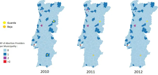
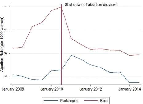
The second instrument is retrieved through a DD regression based on a regional natural experiment using the districts of Beja and Guarda, which from 2011 onwards stopped having an abortion provider.34 Thus the first stage regression will be:
ln(AbortionRatemt)= β0+ β1Be ja+β22011+ β3Be ja×2011+contr olsmt +εmt (9)
All variables are aggregated to the monthly (t) municipal (m) level. The controls included
where time and municipality fixed effects, and the monthly municipal insured unemployment rate per one thousand inhabitants.
The second instrument is closely related to the first. The difference is that it exploits the loss of abortion providers in two of the 18 districts of Portugal: Beja and Guarda. These are the two only cases of loss of abortion providers among regions of such dimension.35 Using the DD regression as a first stage regression is valid, since it is both relevant and exogenous. It is relevant since it is expected that the loss of access to abortion services decreases the number of abortions in the district. It is exogenous since the loss of abortion providers should not affect the access to birth delivery services. The districts used as controls where the ones which were both geographically and culturally similar in order to use comparable units. The Guarda district is as an interior and northern district that is comparable with the districts of Viseu, Castelo Branco, Vila Real and Bragança. Beja can be compared with the districts of Évora and Portalegre since it has a socioeconomic and cultural homogeneity that derives from the fact that these three districts together form the region of Alentejo, a region with a strong cultural identity and similar customs.
34The district of Évora never had any abortion provider. All remaining districts had at least one abortion provider per year.
35More information on the shut-down of these services can be found in Appendix C.
In addition, to employ the DD strategy correctly, the parallel trend assumption must be verified. This assumption is only verified between the districts of Guarda and Castelo Branco and between the districts of Beja and Portalegre, as Figure 2 and 3 in Appendix B show. For this reason the first stage regression will only use these two districts as a control group.
Examining the geographical distribution of abortion centers in Portugal for the years of 2010, 2011 and 2012, represented below in Figure 1, one can clearly see that the south of Portugal had less available options than the north. For this reason, the shutdown of the abortion services of the Hospital of Baixo Alentejo (Beja) is expected to have a higher impact in abortion rates than the shutdown in Guarda, since Beja has clearly less abortion providers nearby than Guarda.
Figure 1: Abortion Providers in the years of 2010, 2011 and 2012
The first stage regressions in table 8 illustrate my previous point. All dependent variables are in logs. The table has the same structure as table 6. In column 1, the DD regression using Guarda and Castelo Branco, the coefficient of the interaction term between Guarda and the year of 2011 has no significant effect on any column meaning, the loss of access did not impact the abortion rate of any age group. Consequently the exogeneity condition is not met and thus we will not instrument the birth rate with the DD of Guarda. As for the first stage regression using the Beja case, displayed in column 2, the coefficient of the interaction term between Beja and the year of 2011 has a significant and negative impact of 16.3% in the abortion rate for the overall birth rate, 15.7% in the abortion rate of women aged younger than 24 and 19.2% on the abortion rate of middle aged women. These coefficients, as in the case regarding the distance instrument, provide ground for the hypothesis that overall, less access leads to less abortions and consequently the loss of the abortion center led to a decrease in the abortion rate of the Beja district.
Table 9, which instruments the DD using the loss of access of the district of Beja shows that the abortion rate has no significant impact on fertility. According to the endogeneity test (GMM distance test) no endogeneity between abortion rates and social outcomes were found using this method.
Table 8: First stage regression: Guarda and Beja’s Difference-in-Differences
Guarda´s Abortion rate Beja´s Abortion rate
(1) (2)
Guarda×2011 -0.0156
(0.0418)
Beja×2011 -0.163∗∗∗
(0.0472)
F statistic 0.139 11.93
F p-value 0.709 0.001
Note: All regressions have municipal and time fixed-effects and include municipal unemploymentper capita.
Robust standard errors in parentheses.
∗p<0.10,∗∗ p<0.05,∗∗∗p<0.01
Table 9: Second stage regressions using Beja Differences-in-Diferences as an instrument of the abortion rate
Birth rate
Abortion rate 0.226
(0.374)
GMM Distance test 0.401
GMM Distance test p value 0.527
Note: All regressions have municipal and time fixed-effects and include municipal unemploy-mentper capita.
Robust standard errors in parentheses.
∗p<0.10,∗∗p<0.05,∗∗∗p<0.01
5.3
Methodological discussion of abortion’s impact on fertility
Our results show that abortion has a negative impact on the fertility rate.
We reached this conclusion even though two of our methodologies (the regression that used the legal status of abortion in Portugal and the regression which employed the DD of Beja as an instrument) yield no significant results. Nevertheless, the regression that uses distance to the nearest provider as an instrument clearly shows a negative impact of abortion rates on overall birth rates with a stronger negative impact in birth rates of women younger than 24 years old. The later is our preferred specification since the regression using the legal status of abortion raises questions about its robustness due to the previously mentioned fact that it uses a very narrow window between different law implementation time-lines (6 months) and to the peculiarities of the region of Portugal considered (Madeira) to build a solid counter-factual. As for the regression using Beja’s DD as an instrument, it was not a robust method since it did not identified any endogeneity between abortion rates and birth rates. As Joyce (2004) suggests that there is in fact endogeneity between abortion rates and birth rates and since we were able to prove this relation through the use of the regression employing distance as an instrument we cannot infer any conclusions using the Beja’s DD regression.
The fact that Portugal legalized abortion as a whole in a short time period allows for several potential confounding trends to hurt the robustness of this analysis, as it is the case of the 2008 economic crisis. Unlike Levine et al. (1999) we could not employ such a robust DD due to the differences between the history of abortion legislation time-lines of implementation in Portugal and the US. Instead we had to assume that the controls we used in our regressions covered all the unobservable effects, without damaging the true effect of legalizing abortion, which it is not possible to assure. It would be of great value if future research on this area manages to better disentangle the drivers of fertility in order to reach a more robust effect of abortion legalization on fertility.
6
Final Discussion
Legal abortion represents a fifth of total birth occurred in the period between 2008 and 2014. Young women, between 15 and 25 years old, represent a larger share of abortions than of births, which shows the weight that the abortion solution still has on the problem of unwanted pregnancy management in this age group, denoting poor contraception insight and/or ineffective pregnancy planning. The opposite happens in women older than 25 years old that have larger shares of births than abortions, revealing maturity in family planning. Our probability model shows exactly that: the younger the woman is the higher is the likelihood to abort once the woman is pregnant.
Not surprisingly abortion is more prevalent in less educated women, which nevertheless does not mean these are more prone to abort. What happens is that Portugal has a larger share of low educated population relatively to the higher educated population and thus it is expected that uneducated women contribute with a higher number of observations. Interestingly, we estimated
that once the woman is pregnant, she has higher odds of aborting if she has a higher level of education. Despite the fact that having lower education might predispose to a more disadvantaged social-economic status and therefore to less resources to raise a family, they however tend to more frequently choose to carry on pregnancy relatively to higher educated women.
As for the woman’s employment status, employed women are simultaneously the major contributors to fertility and abortion, with close to 60% of the share of both births and abortions, representing in one hand a group of women with greater financial stability that enables family growth, but on the other hand they also represent a group of women with a professional career ambitions and responsibilities that might be threatened by the increased family dedication and obligations as well as the labor market pressure and fear of losing their jobs. This is in accordance with our model that predicts that employed women have higher likelihood of choosing to abort.
This higher prevalence regarding both more births and abortions is even stronger among women working in jobs that require a medium level of qualifications and women who’s partner works in a job that requires medium qualifications. Similarly to what was explained in the case of education, medium qualified jobs represent a higher share of nationwide jobs and thus providing more observations than other groups. Regarding our model, the less qualified the job of both the women and the partner is, the higher is the likelihood of aborting. More qualified jobs are associated with more financial stability, which in turn reduces the relative financial weight of having a child.
Living with a partner, mostly if he is employed and with an educational intensive job seems to be a factor that affects positively the decision of giving birth. It is easy to understand that the perspective of being a single-mother is more dissuasive of giving birth relatively to the situation where one has a stable relationship to raise a child. Our model predicts that cohabitation is the strongest factor when it comes to decide whether or not to abort. That allied to the fact of the partner having a job (in particular if the job is educational intensive) enhances the likelihood of giving birth. This shows the importance of both emotional and financial stability on the decision of raising a child.
The addition of one extra element to a family carries with it a financial burden that not all families are able to handle. Our findings reflect this reality. Our model predicts that women who already gave birth are more prone to abort than women who did not, which leads to the conclusion that even in experienced women or experienced families, family planning needs to be reinforced throughout the whole woman’s reproductive age.
Distance also proved to be an important factor in the abortion decision since women who lived farther from abortion centers were less likely to abort. These results raise a question about inter-regional equity.
Finally, living in municipalities that are abortion favorable increases the odds of aborting. As in Ananat et al. (2009), this reduces the social cost of aborting, since it helps to overcome stigma and social pressure. Women living in these areas can also be more likely to be pro-abortion and thus feel fewer moral constraints when they decide whether to abort or not.
Having determined the socio-economic factors that influence the abortion decision, it is
important to refer that abortion decision is multi-factorial and there are more dimensions behind the women decision besides her socioeconomic status, such as her personal beliefs or her life circumstances (Finer et al.2005).
Nevertheless, the elaboration of this probabilistic model allowed to better characterize women who abort. We then focused our analysis in the primary future health indicator of the newborn (LBW) as well as in other indicators related to the infants health (LGA and prematurity) and we related these outcomes to the abortive profile of the pregnant woman.
We found that women with higher odds of giving birth have lower chances of delivering a LBW child. In our view this is one of the key aspects of our study since it provides ground to infer that abortion does induce selection effects regarding this important health indicator. For this reason, our results allow to conclude that abortion leads to positive selection as in the studies of Donohue and Levitt (2001) and Gruber, Levine, and Staiger (1999) found for other outcomes. This study provides evidence that might be used to identify women with modifiable risk factors of social vulnerability and that could benefit from specific support interventions to improve better birth outcomes chances.
As for LGA and prematurity, women with higher odds of giving birth were more likely to deliver children with these outcomes. Since prematurity is frequently idiopathic it is challenging to use this information to identify modifiable risk factors and consequently risk groups. In what concerns LGA and the associated risk of the child’s potential future overweight, obesity, and related co-morbidities, despite of the importance of LGA as a health indicator, there are already intervention programs focusing on diabetic and overweight women in order to reduce the risk of delivering a LGA baby. Therefore our study does not identify new modifiable risks that were not being already addressed.
Having said that, our study suffers from focusing on very short-run outcomes that are influ-enced by several factors that do not necessarily have a socio-economic cause, contrary to outcomes such as criminality or labor market performance. We were constrained in our analysis by the fact that abortion was legalized in 2007, meaning that, at the time of this study, the first birth cohort born in the post-legalization time only has 9 to 10 years of age. Consequently we have a limited number of outcomes to test. Hence, it would be interesting to follow up these children. In the next 5 years these cohorts will be submitted to national exams which will generate new data that might be used to assess the impact of abortion legalization on education. With time increasing information on these children will be available. This population can be used by future studies to test, using other outcome variables, if selection effects do exist and quantify their dimension in case they do.
Regarding our municipal-level analysis, we used three different models to estimate the impact of legalizing abortion on fertility. This strategy was intended to infer the robustness of our estimates. However, due to potential flaws found in two of the methodologies used, we preferred to focus on the model that instruments distance to the nearest abortion provider on the abortion rate since it was the most robust method from the three methods used, due to the reasons previously mentioned in section 5.